Jaynes-Cummings model in a finite Kerr medium

Abstract

We introduce a spin model which exhibits the main properties of a Kerr medium to describe an intensity dependent coupling between a two-level atom and the radiation field. We select a unitary irreducible representation of the $su(2)$ Lie algebra such that the number of excitations of the field is bounded from above. We analyze the behavior of both the atomic and the field quantum properties and its dependence on the maximal number of excitations.

I Introduction

The Jaynes-Cummings model (JCM) 1 is one of the simplest quantum systems describing the interaction of matter with electromagnetic radiation employing a Hamiltonian of a two-level atom coupled to a single bosonic mode. Due to its importance in laser physics and quantum optics, this model has been the subject of many recent investigations, both theoretical and experimental 2 . It has been observed 3 that the temporal behavior of this system is very sensitive to the statistical properties of the radiation field in the initial state, revealing pure quantum features which have no classical counterpart, such as vacuum Rabi oscillations 3A , collapse and revival phenomena 4 and squeezing of the radiation field 4A . These predictions have been verified experimentally 5 .

The JCM has been generalized in different ways. In some cases, the interaction between the atom and the radiation field is no longer linear in the field variables, i.e. intensity dependent coupling has been considered 6 . Other investigations relate the JC Hamiltonian to $u\left(1|1\right)$ and $osp\left(2|2\right)$ superalgebras 7 . Most of the nonlinear generalizations of the JCM are made by using appropriate $q$-deformed oscillators 8 ; 9 . In this framework, the application of the corresponding quantum algebras has proved useful in obtaining exactly soluble models 10 ; 11 . Additional generalizations of the JCM can be found in 11B .

Nonlinear phenomena are ubiquitous in quantum optics. One of the simplest phenomenon is the Kerr effect, which occurs when the refractive index of a medium varies with the number of excitations of the field. Quantum descriptions of optical fields propagating in a Kerr medium reveal a number of interesting features, such as photon antibunching, squeezing and the formation of Schrödinger cats 12 ; 14 , which have no classical analogues. The Kerr medium has been recently considered in the framework of $q$-deformed oscillators 15 and the Moyal phase space representation 16 . Some authors have considered a system where a two-level atom is surrounded by a Kerr medium using a special case of $q$-deformed oscillators 17 .

In this paper, we use an $SU(2)$ spin model, which exhibits the main properties of the Kerr medium 18 , to describe an intensity dependent coupling between a two-level atom and the radiation field in the framework of the JCM. The main feature of the model is that it is formulated on a finite dimensional Hilbert space, so that the number of excitations of the field is bounded from above. In the limit when the dimension of the Hilbert space becomes infinite, the $su\left(2\right)$ algebra of the spin operators contracts to the Heisenberg-Weyl algebra of boson operators and the model coincides with the usual JCM.

II A Kerr Hamiltonian arising from an $SU(2)$ spin system

It is well known that the Heisenberg-Weyl algebra can be obtained by a contraction of the $su\left(2\right)$ algebra 18A . Taking this limit as a motivation, let us start by considering the $su\left(2\right)$ commutation relations

$$[\hat{S}_{+},\hat{S}_{-}]=2\hat{S}_{3},~{}\ [\hat{S}_{3},\hat{S}_{\pm}]=\pm\hat{S}_{\pm},~{}\ \hat{S}_{\pm}=\hat{S}_{1}\pm i\hat{S}_{2}.$$ (1)

In a given unitary irreducible representation $j$, we introduce the operators

$$\hat{b}=\frac{\hat{S}_{-}}{\sqrt{2j}},~{}\ ~{}\hat{b}^{{\dagger}}=\frac{\hat{S}_{+}}{\sqrt{2j}},~{}~{}\ \hat{n}=\hat{S}_{3}+j,$$ (2)

which act on a $\left(2j+1\right)$-dimensional Hilbert space of a particle with spin $j$ 18 . The $su\left(2\right)$ algebra in this representation is thus written as

$$[\hat{b},\hat{n}]=\hat{b},~{}~{}\ [\hat{b}^{{\dagger}},\hat{n}]=-\hat{b}^{{\dagger}},~{}~{}\ [\hat{b},\hat{b}^{{\dagger}}]=1-\frac{\hat{n}}{j},$$ (3)

which allows the interpretation of $b^{\dagger}$ ($b$) as creation (annihilation) operators for the quanta labeled by the number operator $\hat{n}$. The oscillator-like Hamiltonian, in terms of the spin $j$ operators, is 

$$\hat{H}=\frac{\hbar\omega}{4j}(\hat{S}_{+}\hat{S}_{-}+\hat{S}_{-}\hat{S}_{+})=\hbar\omega\left(\hat{n}+\frac{1}{2}-\frac{\hat{n}^{2}}{2j}\right).$$ (4)

The analogy of this expression with the usual optical Kerr Hamiltonian is evident, but the main difference is that the spin number excitation is bounded from above: $n\leq 2j$. This is a consequence of the angular momentum condition $-j\leq m\leq+j$, once it is written in terms of the eigenvalues of the number operator $\hat{n}$. Clearly the energy spectrum has the twofold degeneracy $E\left(n\right)=E\left(2j-n\right)$. Note that although this Hamiltonian can be easily obtained in the framework of $q$-deformed oscillators, we use an algebraic model which possesses a physical interpretation of quantum deformation based on the fundamental $SU\left(2\right)$ group. The standard harmonic oscillator limit is obtained when $j\rightarrow\infty$, in which case $\hat{b}$ and $\hat{b}^{{\dagger}}$ turn out to be  the usual bosonic operators acting on an infinite dimensional Hilbert space, i.e., the nonlinearity and the maximum number of excitations disappear. We observe that the relation between the number operator and the corresponding creation-annihilation operators is 

$$\hat{n}=\frac{(2j+1)}{2}\left[1-\sqrt{1-\frac{8j}{(2j+1)^{2}}\hat{b}^{{\dagger}}b}\right],$$ (5)

which leads to the usual relation $\hat{n}=\hat{b}^{{\dagger}}b$ when $j\rightarrow\infty$.

The solution of Heisenberg’s equation of motion for spin operators is

$$\hat{S}_{1}(t) = e^{i\frac{\omega t}{2j}}[\cos(\hat{\Omega}t)\hat{S}_{1}-\sin(\hat{\Omega}t)\hat{S}_{2}],$$

$$\hat{S}_{2}(t) = e^{i\frac{\omega t}{2j}}[\sin(\hat{\Omega}t)\hat{S}_{1}+\cos(\hat{\Omega}t)\hat{S}_{2}],$$

$$\hat{S}_{3}(t) = \hat{S}_{3},$$ (6)

where $\hat{\Omega}=\omega(1-\frac{\hat{n}}{j})$. Thus, the time evolution of $\vec{S}\left(t\right)$ is a rotation around the $z$ axis, but the precession frequency depends on the excitation number operator. This result is in complete analogy with that obtained in the case of the Kerr medium 19 ; 20 .

In molecular physics, this model correspond to a diatomic molecule approximated by a Morse potential and the eigenstates correspond to the $U(2)\supset SU(2)$ symmetry-adapted basis 21 ; 22 . It was shown that this type of Hamiltonian describes the interaction of a collective atomic system with the off-resonant radiation field in a dispersive cavity 23 .

III SU(2) Coherent states

Nonlinear coherent states (NCSs) have been discussed in different approaches and arriving to different states 24 ; 25 . The most representative ones are constructed  in the framework of $q$-deformed oscillators 26 , in which NCSs are eigenstates of the $q$-annihilation operator. A generalization of the $SU(2)$ coherent states given by a multiphoton Holstein-Primakoff transformation is discussed in Ref.26A , and their physical consequences are studied in the framework of the standard JC model. Here we describe the $SU(2)$ coherent states corresponding to the single photon case in the SU(2) spin model and use them to study the modified JC model to be defined in the next section.

The group-theoretical coherent state (see ref.23A ) for the unitary irreducible representation of the $su(2)$ Lie algebra corresponding to Eq.(2) is:

$$\left|\alpha\right\rangle=e^{\alpha\hat{S}_{+}-\alpha^{\ast}\hat{S}_{-}}\left|j,-j\right\rangle,$$ (7)

where $\alpha=\frac{\theta}{2}e^{-i\phi}$, $0\leq\theta\leq\pi$, $0\leq\phi\leq 2\pi$ and the ladder operators $\hat{S}_{\pm}$ select the vacuum state $\left|0\right\rangle$ from the states $\left|j,m\right\rangle$ as usual: $\hat{S}_{-}\left|0\right\rangle=\hat{S}_{-}\left|j,-j\right\rangle=0$. The natural phase space is the sphere of radius $j$; the spin coherent states are thus represented by spots on the sphere. This dynamics leads to Schrödinger cat states on the sphere 18 , i.e., a superposition of several spots located “far” from each other. In the harmonic limit, the sphere opens to the phase plane and the model coincides with the quantum harmonic oscillator or, through a renormalization, with the usual Kerr medium.

Using the disentangling theorem for $SU(2)$ operators, we can rewrite Eq.(7) in the following form

$$\left|\xi\right\rangle=(1+\left|\xi\right|^{2})^{-j}\sum_{m=-j}^{+j}\left(\begin{array}[]{c}2j\\ j+m\end{array}\right)^{\frac{1}{2}}\xi^{\left(j+m\right)}\left|j,m\right\rangle,\;\;\;$$ (8)

where $\xi=\tan\left(\frac{\theta}{2}\right)e^{-i\phi}$. Then, the photon number distribution of the field prepared in the state $\left|\xi\right\rangle$ is

$$\mathcal{P}_{n}\left(\left|\xi\right|^{2}\right)=\left(\begin{array}[]{c}2j\\ n\end{array}\right)\frac{\left|\xi\right|^{2}}{\left(1+\left|\xi\right|^{2}\right)^{2j}},$$ (9)

and the mean photon number is

$$\left\langle\hat{n}\right\rangle=2j\frac{\left|\xi\right|^{2}}{1+\left|\xi\right|^{2}}.$$ (10)

This result shows that $\left\langle\hat{n}\right\rangle$ is bounded from above. It is convenient to rewrite Eq. (9) in the following form

$$\mathcal{P}_{n}\left(\chi\right)=\left(\begin{array}[]{c}2j\\ n\end{array}\right)\chi^{n}\left(1-\chi\right)^{2j-n},$$ (11)

which is a binomial distribution in $n$ with parameter $\chi\equiv\frac{\left\langle\hat{n}\right\rangle}{2j}\in\left[0,1\right]$. Evidently $\mathcal{P}_{n}\left(\chi\right)$ converges towards the Poisson distribution if $\left\langle\hat{n}\right\rangle$ remains fixed when $2j\rightarrow\infty$. One of the most interesting features of the $SU(2)$ coherent states is that they exhibit squeezing which depends on $2j$.

IV Two-level atom surrounded by a Kerr medium.

We start with a brief review of the standard formulation of the JCM. In the dipole and rotating wave approximation, the JC Hamiltonian for a system of a single atom interacting with a single mode is given by 1

$$\mathcal{H}_{JC}=\frac{1}{2}\hbar\omega(\hat{a}^{{\dagger}}\hat{a}+\hat{a}\hat{a}^{{\dagger}})+\frac{1}{2}\hbar\omega_{0}\hat{\sigma}_{3}+\hbar\lambda(\hat{\sigma}_{+}\hat{a}+\hat{a}^{{\dagger}}\hat{\sigma}_{-}),$$ (12)

where $\frac{1}{2}\hbar\omega(\hat{a}^{{\dagger}}\hat{a}+\hat{a}\hat{a}^{{\dagger}})$ and $\frac{1}{2}\hbar\omega_{0}\hat{\sigma}_{3}$ are the well-known energy operators for the field and atom, respectively. Here $\omega$ is the field mode frequency and $\omega_{0}$ is the atomic transition frequency. The coupling between the atom and the radiation field is described by $\hbar\lambda(\hat{\sigma}_{+}\hat{a}+\hat{a}^{{\dagger}}\hat{\sigma}_{-})$, where $\lambda$ is a coupling constant. Besides $\hat{a}$ and $\hat{a}^{{\dagger}}$ are the usual bosonic creation and annihilation operators for photons in the mode, which obey the Heisenberg-Weyl algebra. $\hat{\sigma}_{+}$ and $\hat{\sigma}_{-}$ are the usual rising and lowering operators describing the fermionic two-level atom and $\hat{\sigma}_{3}$ is the atomic inversion operator, which follow the standard pseudo-spin algebra.

Now, let us introduce the spin model discussed in Sec. II into the JC Hamiltonian to describe a two-level atom surrounded by a Kerr medium. This is achieved by replacing the usual bosonic creation and annihilation operators by the correspondent spin-$j$ operators, i.e. we now consider

$$\mathcal{H}_{JC}=\frac{1}{4j}\hbar\omega(\hat{S}_{+}\hat{S}_{-}+\hat{S}_{-}\hat{S}_{+})+\frac{1}{2}\hbar\omega_{0}\hat{\sigma}_{3}+\frac{\hbar\lambda}{\sqrt{2j}}(\hat{\sigma}_{+}\hat{S}_{-}+\hat{S}_{+}\hat{\sigma}_{-}).$$ (13)

Next, we will concentrate on studying the dynamics of the system. We first split the Hamiltonian into two parts : $\mathcal{H}_{0}$ (the energy operator in the absence of interaction) and $\hat{\mathcal{V}}$ (the coupling interaction), such that

$$\mathcal{H}_{JC}=\mathcal{H}_{0}+\hat{\mathcal{V}},$$ (14)

where

$$\mathcal{H}_{0} = \frac{1}{4j}\hbar\omega(\hat{S}_{+}\hat{S}_{-}+\hat{S}_{-}\hat{S}_{+})+\frac{1}{2}\hbar\omega_{0}\hat{\sigma}_{3},$$ (15)

$$\hat{\mathcal{V}} \mathcal{=} \frac{\hbar\lambda}{\sqrt{2j}}(\hat{\sigma}_{+}\hat{S}_{-}+\hat{S}_{+}\hat{\sigma}_{-}).$$ (16)

In the interaction picture generated by $\mathcal{H}_{0}$, the Hamiltonian of the system is

$$\hat{\mathcal{V}}_{\mathcal{I}}\left(t\right)=e^{i\frac{\mathcal{H}_{0}t}{\hbar}}\hat{\mathcal{V}}e^{-i\frac{\mathcal{H}_{0}t}{\hbar}}.$$ (17)

It is clear that $\hat{\sigma}_{\pm}$ and $\hat{S}_{\pm}$ become time-dependent by means of the Heisenberg equations of motion. Then the interaction picture Hamiltonian becomes

$$\hat{\mathcal{V}}_{\mathcal{I}}\left(t\right)=\frac{\hbar\lambda}{\sqrt{2j}}{(\hat{\sigma}}_{+}e^{i\hat{\Omega}_{\hat{n}}t}\hat{S}_{-}+\hat{S}_{+}e^{-i\hat{\Omega}_{\hat{n}}t}\hat{\sigma}_{-}),$$ (18)

where

$$\hat{\Omega}_{\hat{n}}=\omega_{0}-\omega\left(1-\frac{\hat{n}}{j}-\frac{1}{2j}\right)$$ (19)

gives rise to the generalized detuning frequency, which depends on the excitation number operator.

In order to solve the equation of motion in the interaction picture, we first observe that $\hat{\mathcal{V}}_{\mathcal{I}}$ describes processes where a photon in the mode is annihilated while the atom is excited, or vice versa. Then, at any time $t$, the state of the system $\left|\psi\left(t\right)\right\rangle$ is expanded in terms of the states $\left|n\right\rangle\otimes\left|+\right\rangle$ and $\left|n+1\right\rangle\otimes\left|-\right\rangle$, where $\left|n\right\rangle$ is an eigenstate of the excitation number operator and $\left|+\right\rangle$ and $\left|-\right\rangle$ denote the atom in the excited and ground state, respectively. Thus

$$\left|\psi\left(t\right)\right\rangle=\sum_{n=0}^{2j}\left[a_{n}\left(t\right)\left|n\right\rangle\otimes\left|+\right\rangle+b_{n}\left(t\right)\left|n+1\right\rangle\otimes\left|-\right\rangle\right].$$ (20)

The equation of motion for the state of the system in the interaction picture, i.e. $i\hbar\frac{\partial}{\partial t}\left|\psi\left(t\right)\right\rangle=\hat{\mathcal{V}}_{\mathcal{I}}\left(t\right)\left|\psi\left(t\right)\right\rangle$, gives the following simple coupled set of differential equations for the probability amplitudes

$$i\dot{a}_{n} = \lambda\sqrt{\left(n+1\right)\left(1-\frac{n}{2j}\right)}e^{i\Omega_{n}t}b_{n},$$ (21)

$$i\dot{b}_{n} = \lambda\sqrt{\left(n+1\right)\left(1-\frac{n}{2j}\right)}e^{-i\Omega_{n}t}a_{n},$$ (22)

whose general solution is

$$a_{n}\left(t\right)=\left\{a_{n}\left(0\right)\left[\cos\left(\frac{\Gamma_{n}t}{2}\right)-i\frac{\Omega_{n}}{\Gamma_{n}}\sin\left(\frac{\Gamma_{n}t}{2}\right)\right]-ib_{n}\left(0\right)\sqrt{1-\frac{\Omega_{n}^{2}}{\Gamma_{n}^{2}}}\sin\left(\frac{\Gamma_{n}t}{2}\right)\right\}e^{i\Omega_{n}t},$$

$$b_{n}\left(t\right)=\left\{b_{n}\left(0\right)\left[\cos\left(\frac{\Gamma_{n}t}{2}\right)+i\frac{\Omega_{n}}{\Gamma_{n}}\sin\left(\frac{\Gamma_{n}t}{2}\right)\right]-ia_{n}\left(0\right)\sqrt{1-\frac{\Omega_{n}^{2}}{\Gamma_{n}^{2}}}\sin\left(\frac{\Gamma_{n}t}{2}\right)\right\}e^{-i\Omega_{n}t},$$

where $a_{n}\left(0\right)$ and $b_{n}\left(0\right)$ are determined from the initial conditions of the system and

$$\Gamma_{n}=\sqrt{\Omega_{n}^{2}+4\lambda^{2}\left(n+1\right)\left(1-\frac{n}{2j}\right)}$$ (24)

is the generalized Rabi frequency.

This set of equations gives us the general solution of the problem. In order to calculate some physical quantities of interest, we still need to specify the initial photon number distribution of the field.

Exact solutions of generalized extensions of the JCM in the Schrödinger picture have been calculated in Ref.11B . Our modified algebra (Eq.3) is also included in this generalization with the appropriate choice of the structure functions. Unlike this approach, here we use a unitary irreducible representation of the $su(2)$ algebra to describe a Kerr medium, taking advantage of algebraic methods. In addition, we now explore the physical consequences of the model.

V Quantum properties

Since the JCM is a composite system, which includes the field and the atom sectors, the quantum properties can be described using the joint density operator

$$\hat{\rho}_{\mathcal{AF}}\left(t\right)=\left|\psi\left(t\right)\right\rangle\left\langle\psi\left(t\right)\right|,$$ (25)

where the subscript $\mathcal{A}$ and $\mathcal{F}$ refers to the atom and the field contributions.

The reduced density operators are then sufficient for calculating the averages of any dynamical variables that belong exclusively to one of the components. The reduced density operators are

$$\hat{\rho}_{\mathcal{A}}\left(t\right)=Tr_{\mathcal{F}}\left[\hat{\rho}_{\mathcal{AF}}\left(t\right)\right],~{}\ \ \ \hat{\rho}_{\mathcal{F}}\left(t\right)=Tr_{\mathcal{A}}\left[\hat{\rho}_{\mathcal{AF}}\left(t\right)\right],$$ (26)

with which we are able to evaluate the expectation values of any atomic operator $\mathcal{O}_{\mathcal{A}}$ (e.g. population inversion operator $\hat{\sigma}_{3}$) and of any field operator $\mathcal{O}_{\mathcal{F}}$ (e.g. excitation number operator $\hat{n}$) using the expressions

$$\left\langle\mathcal{O}_{\mathcal{A}}\right\rangle=Tr_{\mathcal{A}}\left[\hat{\rho}_{\mathcal{A}}\left(t\right)\mathcal{O}_{\mathcal{A}}\right],~{}\ \ \left\langle\mathcal{O}_{\mathcal{F}}\right\rangle=Tr_{\mathcal{F}}\left[\hat{\rho}_{\mathcal{F}}\left(t\right)\mathcal{O}_{\mathcal{F}}\right].$$ (27)

The matrix density of the atom has dimension two and, unlike the usual JCM, the matrix density of the field has dimension $(2j+1)$.

V.1 Atomic population inversion

Many interesting atomic quantum effects have been observed in the context of the standard JCM. Perhaps the most notable is the periodic transfer of population between the ground state and the excited state. These transitions constitute  the so-called collapse and revival phenomena (CR). Physically, CR occur because an atom within a cavity undergoes reversible spontaneous emission, as it repeatedly emits and then reabsorbs radiation 27 .

The general expression for the atomic population inversion is

$$\left\langle\hat{\sigma}_{3}\left(t\right)\right\rangle=Tr_{\mathcal{A}}\left[\hat{\rho}_{\mathcal{A}}\left(t\right)\hat{\sigma}_{3}\right]=\sum_{n=0}^{2j}\left[\left|a_{n}\left(t\right)\right|^{2}-\left|b_{n}\left(t\right)\right|^{2}\right],$$ (28)

where we have used  Eq. (27). We can see that the temporal evolution of $\left\langle\hat{\sigma}_{3}\left(t\right)\right\rangle$ is essentially a result of a summation of probabilities at different Rabi frequencies.

In order to compare the differences between the usual treatment and the spin model, let us consider the atom initially in the excited state and the initial photon number distribution described by the$\;SU\left(2\right)$ coherent states, i. e. $\left|b_{n}\left(0\right)\right|^{2}=0$ and $\left|a_{n}\left(0\right)\right|^{2}=\mathcal{P}_{n}\left(\chi\right)$. Thus

$$\left\langle\hat{\sigma}_{3}\left(t\right)\right\rangle=\sum_{n=0}^{2j}\left(\begin{array}[]{c}2j\\ n\end{array}\right)\chi^{n}\left(1-\chi\right)^{2j-n}\left[\frac{\Omega_{n}^{2}}{\Gamma_{n}^{2}}+\left(1-\frac{\Omega_{n}^{2}}{\Gamma_{n}^{2}}\right)\cos\left(\Gamma_{n}t\right)\right].$$ (29)

We observe that this solution converges towards the usual solution of JCM as $2j$ approaches infinity, i.e. when the $su\left(2\right)$ algebra contracts to the Heisenberg-Weyl algebra. Simultaneously, the photon number distribution of the field converges towards the Poisson distribution when $2j\chi$ remains fixed.

It is well known that the system under consideration is sensitive to the statistical properties of the electromagnetic field. In the $q$-deformed extensions of the JCM, it is usually considered that the field is initially prepared in a $q$-deformed coherent state (an eigenstate of the $q\,$-deformed annihilation operator). On the other hand, in Ref.11B the field is prepared in the multipothon Holstein-Primakoff $SU(2)$ coherent state in the framework of the standard JCM. In this work we consider both situations: an $SU(2)$ spin model to describe an intensity dependent coupling, together with its associated coherent state as the initial photon number distribution.

Figure 1: Plot of the temporal evolution of the atomic inversion $\left\langle\hat{\sigma}_{3}\left(t\right)\right\rangle$ in the standard JCM in the exact resonant case. The atom is initially in the excited state and the field is initially prepared in the standard coherent state with $\left\langle\hat{n}\right\rangle=20$ photons on average.

Numerical results of the atomic inversion in the exact resonant case $\left(\omega=\omega_{0}=\lambda\right)$, with $\left\langle\hat{n}\right\rangle=20$ photons on average and$\;2j\rightarrow\infty$, are shown in Fig. 1. It can be seen that the temporal evolution exhibits periodic collapses and revivals. This phenomenon also takes place in the spin model; however, in this case the structure is more complex due to its dependence on the maximum number of spin excitations $2j$. Figures (2a), (2b) and (2c) show the temporal evolution of $\left\langle\hat{\sigma}_{3}\left(t\right)\right\rangle$ for $\left\langle\hat{n}\right\rangle=20$ photons on average and $2j=1000,~{}100$ and$~{}50$, respectively. We observe in Fig. 2a that the sequence of CR is essentially the same as in the limiting case (Fig. 1), but the scaled time $\lambda t_{R}$ needed for the largest revival of the initial value $\left\langle\hat{\sigma}_{3}\left(0\right)\right\rangle$ depends on the maximum occupation $2j$. An estimate of the scaled time ($2j>>1$) in this case gives

$$\lambda t_{R}\approx\frac{\pi}{\sqrt{\chi^{2}+\left(2+2j\chi\right)\left(1-\chi\right)}-\sqrt{\chi^{2}+\left(1+2j\chi\right)\left(1-\chi\right)}},$$ (30)

which agrees with the numerical results. It can be seen that when $2j$ decreases the structure starts to deteriorate (see Fig. (2b) and (2c)). Due to the symmetry of the photon number distribution, i.e. $\mathcal{P}_{n}\left(\chi\right)=\mathcal{P}_{2j-n}\left(1-\chi\right)$, periodic collapses and revivals also take place for any value of $\chi$, except for the limiting case $\chi=1$. In this case, which does not occur in the standard JCM, the leading term in the sum of Eq.(29) is that for which $n=2j$ and therefore $\left\langle\hat{\sigma}_{3}\left(t\right)\right\rangle=1$, i.e. the atom remains in the excited state.

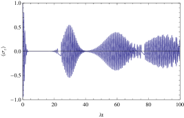
(a)

(b)

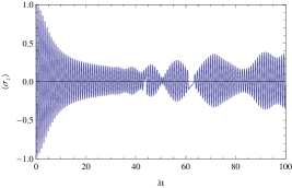
(c)

Figure 2: Plots of the temporal evolution of the atomic inversion $\left\langle\hat{\sigma}_{3}\left(t\right)\right\rangle$ in the spin model in the exact resonant case. The atom is initially in the excited state and the field is initially prepared in the $SU(2)$ coherent state with $\left\langle\hat{n}\right\rangle=20$ photons on average. Frames a), b) and c) correspond to $2j=1000,100$ and $50$ maximum number of excitations, respectively

V.2 Photon antibunching

Both theoretically and experimentally, there is an interest in a variety of statistical properties of the electromagnetic field, including the distributions of possible field energies, the photon number variance and the Mandel $\mathcal{Q}$ parameter (normalized second factorial moment) 28 :

$$\mathcal{Q}\left(t\right)=\frac{\left\langle\left(\Delta\hat{n}\right)^{2}\right\rangle-\left\langle\hat{n}\right\rangle}{\left\langle\hat{n}\right\rangle}.$$ (31)

These statistical variables offer quantitative measures of how much the field differs from a classical field. In particular, the Mandel $\mathcal{Q}$ parameter vanishes for a Poissonian distribution. It provides information about the tendency of photons to arrive in bunches: when $\mathcal{Q}>0$ the photons are bunched (super-Poisson), while for $\mathcal{Q}<0$ the photons are antibunched (sub-Poisson) 27 . It is well know that a sub-Poissonian statistics is a signature of the quantum nature of the field.

Averages appearing in Eq.(31) can be obtained easily from Eq.(27). From figure 3(a) we can see that the photon number distribution oscillates between sub-Poissonian and super-Poissonian statistics when $2j>>1$. Figures 3(b) and (c) show that as $2j$ decreases, $\mathcal{Q}$ becomes negative and the photons are antibunched. From these results we infer the purely quantum regime of the spin model for the electromagnetic field.

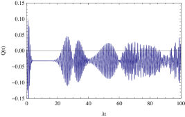
(a)

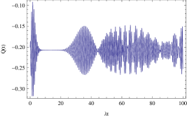
(b)

(c)

Figure 3: Plots of the temporal evolution of the Mandel $\mathcal{Q}\left(t\right)$ parameter in the spin model in the exact resonant case. The atom is initially in the excited state and the field is initially prepared in the $SU(2)$ coherent state with $\left\langle\hat{n}\right\rangle=20$ photons on average. Frames a), b) and c) correspond to $2j=1000,100$ and $50$ maximum number of excitations, respectively

V.3 Squeezing

To analyze the squeezing properties of the radiation field we introduce two hermitian quadrature operators:

$$\hat{x}=\frac{\hat{J}_{x}}{\sqrt{2j}}\text{, \ \ \ \ \ \ \ \ \ \ \ }\hat{y}=\frac{\hat{J}_{y}}{\sqrt{2j}}\text{.}$$ (32)

One of the consequences of the commutation relation for these operators is the uncertainty relation $\left\langle\left(\Delta\hat{x}\right)^{2}\right\rangle\left\langle\left(\Delta\hat{y}\right)^{2}\right\rangle\geq\left|\frac{{\hbar}^{2}}{4}\left(1-\frac{\left\langle\hat{n}\right\rangle}{j}\right)\right|^{2}$. When either of these variances is less than $\frac{{\hbar}^{2}}{4}$ (uncertainty associated with the coherent field, including the vacuum), the state is said to be squeezed 29 ; 30 . In the usual JCM, the cavity field surrounding a two-level atom initially excited, exhibits a time-varying pattern of squeezing both in the short time regime and during the revivals 4A ; 32 . Thus the dynamics of the JCM leads to the squeezing of the radiation field, although the effect is rather weak.

The variances of the quadrature operators can be expressed through the mean values of the spin operators

$$\left\langle\left(\Delta\hat{x}\right)^{2}\right\rangle = \frac{1}{2j}\left[\frac{1}{2}\mathrm{{Re}\left\langle\hat{J}_{+}\hat{J}_{-}\right\rangle+\frac{1}{2}{Re}\left\langle\hat{J}_{+}^{2}\right\rangle-\left({Re}\left\langle\hat{J}_{+}\right\rangle\right)^{2}}\right]\text{,}$$ (33)

$$\left\langle\left(\Delta\hat{y}\right)^{2}\right\rangle = \frac{1}{2j}\left[\frac{1}{2}\mathrm{{Re}\left\langle\hat{J}_{+}\hat{J}_{-}\right\rangle-\frac{1}{2}{Re}\left\langle\hat{J}_{+}^{2}\right\rangle-\left({Im}\left\langle\hat{J}_{+}\right\rangle\right)^{2}\,\,}\right]\text{.}$$

In figure 4 we plot the temporal evolution of the uncertainties as a function of the scaled time. We observe in figure 4(a) that $\left\langle\left(\Delta\hat{x}\right)^{2}\right\rangle$ exhibits squeezing periodically in both cases, for $2j=1000$ (blue line) and $50$ (red line) maximum number of excitations. In figure 4(b) it can be seen that $\left\langle\left(\Delta\hat{y}\right)^{2}\right\rangle$ is larger than the minimum even at $t=0$. On the other hand, figures 4(c) and (d) show that in the longer time behavior the uncertainties remain bounded in both cases (for $2j=1000$ and $50$) . However, they always remain significantly larger than the minimum value and thus the field is no longer squeezed.

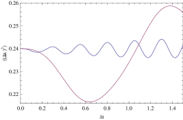
(a)

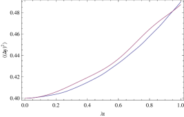
(b)

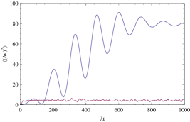
(c)

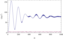
(d)

Figure 4: Temporal evolution of the uncertainties as a function of the scaled time. Frames a) and b) show the short time regime of $\left\langle\left(\Delta\hat{x}\right)^{2}\right\rangle$ and $\left\langle\left(\Delta\hat{y}\right)^{2}\right\rangle$, respectively. In the same order, frames c) and d) show the longer time behavior. The atom is initially in the excited state and the field is initially prepared in the $SU(2)$ coherent state with $\left\langle\hat{n}\right\rangle=20$ photons on average. The maximum number of excitations are $2j=1000$ (blue line) and $2j=50$ (red line).

VI Conclusions

In this work we have introduced a spin model which exhibits the main properties of a Kerr medium to describe an intensity dependent coupling between a two-level atom and the radiation field. The model is formulated in terms of spin operators acting on a finite dimensional Hilbert space, so that the number of excitations of the field is bounded from above. We have analyzed the behavior of both the atomic and the field quantum properties when the atom is initially in the excited state and the field is initially prepared in the $SU\left(2\right)$ coherent state in the exact resonant case.

It has been shown that the atomic population inversion exhibits periodic collapses and revivals when $2j\gg 1$, while with decreasing $2j$ the structures start to deteriorate. When the mean photon number is maximal ($\chi=1$), the atom remains in the excited state. As regards to the quantum properties of the field, we showed that the photon number distribution oscillates between sub-Poissonian and super-Poissonian statistics when $2j>>1$, while as $2j$ decreases $\mathcal{Q}$ becomes negative and the photons are antibunched. In the same fashion, we find squeezing only in the short time regime. We are currently exploring applications of a field-theoretical extension of these ideas 33 .

References

- (1) E. T. Jaynes and F. W. Cummings, Proc. IEEE 51, 89 (1963).
- (2) Moya-Cessa H, Buzek V, Kim M S and Knight P L 1993 Phys.Rev. A 48 3900, S. Stenholm, Phys. Rep. 6, 1 (1973).
- (3) J. H. Eberly, N. B. Narozhny, and J. J. Sanchez-Mondragon, Phys. Rev. Lett. 44, 1323 (1980); N. B. Narozny, J. J. Sanchez, and J. H. Eberly, Phys. Rev. A 23, 236 (1981).
- (4) J. J. Sánchez , N. B. Narozhny and J. H. Eberly, 1983, Phys. Rev .Lett ., 51, 550.
- (5) P. Meystre and M. S. Zubairy, Phys. Lett. 89A, 390 (1982); C. C. Gerry, Phys. Rev. A 37, 2683 (1988).
- (6) P. Meystre and M. S. Zubairy, “Squeezed states in the Jaynes-Cummings model”, Phys. Lett. A, 89, 390, 1982.
- (7) Rempe G and Walther H 1987 Phys. Rev. Lett. 58 353.
- (8) B. Buck and C. V. Sukumar, Phys. Lett. 83A, 132 (1981).
- (9) C. Buzano, M. G. Rasetti and M. L. Rastello, Phys . Rev. Lett. 62, 137 (1989).
- (10) L. C. Biedenharn, J. Phys. A 22, L873 (1989).
- (11) A. J. Macfarlane, J.Phys. A 22, 4581 (1989).
- (12) M. Chaichian, D. Ellinas and P. Kulish, Phys. Rev. Lett. Vol. 60, No. 6, pp.980-983, 1990.
- (13) J. Crnugelj, M. Martinis,and V. Mikuta-Martinis, Phys. Rev. A, Vol. 50, No. 2, 1994.
- (14) D. Bonatsos, C. Daskaloyannis and G. A. Lalazissis, Phys. Rev. A 47(1993)3448.
- (15) Agarwal, G.S., Squeezing in two photon absorption from a strong coherent beam. Opt. Commun. (1987) 62 190-192.
- (16) Ritze, H.H. and Bandilla, A., Quantum effects of a nonlinear interferometer with a kerr cell. Opt. Commun. (1979) 29 126-130.
- (17) Agarwal, G.S. and Puri, R.R., Quantum theory of propagation of elliptically polarized light through a Kerr medium. Phys. Rev. A (1989) 40 5179-5186.
- (18) Man’ko V I, Marmo G and Zaccaria F 2010 Phys. Scr. 81 045004.
- (19) Osborn T A and Karl-Peter M 2009 J. Phys. A: Math. Theor. 42 415302.
- (20) O. de los Santos-Sánchez and J. Récamier, J. Phys. B: At. Mol. Opt. Phys. 45 (2012) 015502.
- (21) Sergey M. Chumakov, Alejandro Frank and Kurt Bernardo Wolf, Phys. Rev. A 60, No.3, 1999.
- (22) Andrei B. Klimov and Sergei M. Chumakov, A Group-Theoretical Approach to Quantum Optics: Models of Atom-Field Interactions (Wiley-VCH, Weinheim, 2009).
- (23) G. S. Agarwal, R. R. Puri, and R. P. Singh, Phys. Rev. A 56, 2249 (1997).
- (24) R. Tanas, in Coherence and Quantum Optics V, edited by L.Mandel and E. Wolf (Plenum, New York, 1984), p. 645.
- (25) A. Frank and P. Van Isacker, Algebraic Methods in Molecular and Nuclear Structure (Wiley Interscience, New York, 1994).
- (26) F. Iachello and A. Arima, The interacting Boson Model (CUP 1987).
- (27) G. J. Milburn, Phys. Rev. A 33, 674 (1986); G. J. Milburn and C. A. Holmes, ibid. 44, 4704 (1991).
- (28) J. M. Radcliffe, J. Phys. A4, 313 (1971).
- (29) Barut A O and Girardello L 1971 Commun. Math. Phys. 21 41.
- (30) Nieto M and Simmons L M 1978 Phys. Rev. Lett. 41 207.
- (31) O de los Santos-Sánchez and J Récamier 2011 J. Phys. A: Math. Theor. 44 145307.
- (32) V. Buzek and I. Jex, J. Mod. Optics 36(1989)1427.
- (33) Shore, Bruce W. and Knight, Peter L. (1993), Journal of Modern Optics, 40: 7 1195-1238.
- (34) L. Mandel, “Sub-Poissonian photon statistics in resonance fluorescence”, Optics Lett., 4, 205, 1979.
- (35) R. E. Slusher and B. Yurke, “Squeezed states generation experiments in an optical cavity”, Frontiers of Quantum Optics, edited by E.R. P ike and S. Sarker (Bristol: Adam Hilger), pp.41, 1986.
- (36) R. Loudon and P. L. Knight, “Squeezed light”, J. Mod. Optics, 34, 709, 1987.
- (37) K. Wodkiewicks, P. L. Knight, S. J. Buckle and S. M. Banett, “Squeezing and superposition states”, Phys. Rev. A, 35, 2567, 1987.
- (38) A. Martín Ruiz, L. F. Urrutia and Alejandro Frank, in preparation.