A Universal Quantum Circuit Scheme For Finding Complex Eigenvalues
Abstract
We present a general quantum circuit design for finding eigenvalues of non-unitary matrices on quantum computers using the iterative phase estimation algorithm. In addition, we show how the method can be used for the simulation of resonance states for quantum systems.
Keywords:
Quantum Circuits Quantum Algorithms Phase Estimation Complex Eigenvalues Resonance States1 Introduction
In the circuit model of quantum computation, a controlled quantum system, considered to be a quantum computer, propagates from one state to another through the application of a local propagator called a quantum gate. A given algorithm, or computation, can be implemented on a quantum computer using a sequence of quantum gates. These gates can be represented by unitary matrices in the computational basis. While this unitary representation is adequate for many problems, it impedes application of quantum computing to new problems, where computations can only be described through non-unitary matrices. Furthermore, any attempt at approximation of these non-unitary parts negatively impacts the accuracy of the results. For instance, the algorithm of Harrow et. al Lloyd for solving linear systems of equations requires a non-unitary quantum gate. The circuit designed for this algorithm Yudong uses an approximated gate for the non-unitary parts.
Quantum algorithms are known to be more efficient than their classical counterparts Deutsch ; Bennett ; Delgado . They often provide exponential efficiency gains for the simulation of quantum systems Abrams ; Papageorgiou . The idea of making a computer compatible, from the start, with the principles of quantum theory for simulations of quantum systems was discussed in 1969 by Finkelstein Finkelstein . Later in 1981, Feynman Feynman explained why it is impossible to simulate a quantum system using a probabilistic classical computer. He also described a universal quantum computer capable of simulating quantum physics. Since then, different algorithms and quantum circuit designs have been proposed for the simulation of various quantum systems – simulation of chemical dynamics Sanders2009algorithm ; Sanders ; Kassal2008polynomial , simulation of sparse Hamiltonians Berry2007 , calculating the thermal rate constant New3 , and others Brown2010 ; New6 ; Kassal2011 ; Whaley2012 . Arguably, the most important one of these algorithms is the phase estimation algorithm Abrams ; Kitaev , used for finding the eigenvalues of a given unitary matrix, or equivalently, the eigen-energies of the corresponding quantum system. The algorithm has been applied in quantum chemistry to obtain energies of molecular systems New1 ; New2 ; New4 ; Daskin2 . The algorithm has also been demonstrated experimentally for the simulation of the hydrogen molecule using photonic New5 ; Alan2012 and NMR quantum computers New6 ; Du2010 . One of the postulates of quantum mechanics states that measurable quantities such as the energy of stable atoms and molecules are real quantities and the operator that represents them should be a Hermitian operator. Because the eigenvalues of Hermitian operators are real, the expectation of any measurable quantity related to these eigenvalues is also real. However, it is almost impossible to obtain the poles of the scattering matrix within the framework of the standard formalism of the quantum mechanics, where we use only Hermitian operators. In the non-Hermitian formalism, the poles of the scattering matrix can be directly calculated from the complex eigenvalues of the non-Hermitian Hamiltonian Moiseyev2011 . The simulation of non-Hermitian matrices in quantum theory requires the simulation of non-unitary evolution matrices. However, quantum computers are based on the standard formalism; hence, computations are done using unitary evolution operators.
It has been shown that a quantum circuit can be generalized to a non-unitary circuit, whose constituents are non-unitary gates representing quantum measurement. Furthermore, it is shown that a specific type of one-qubit non-unitary gates, the controlled-NOT gate, and all one-qubit unitary gates constitute a universal set of gates for the non-unitary quantum circuit without the necessity of introducing ancilla qubits Terashima . Recently, Wang et al. Hefeng-MPEA , proposed a measurement-based quantum algorithm for finding eigenvalues of non-unitary matrices. Their method draws on ideas from conventional phase estimation algorithm, frequent measurement, and techniques in one-qubit state tomography. They describe a bipartite system composed of two subsystems, where the total Hamiltonian includes the Hamiltonians of each subsystem and their interaction. They show that different non-unitary evolution matrices can be constructed by performing sequential projective measurements on one of these subsystem. In addition, they show that an eigenvalue of the constructed matrix can be estimated within the phase estimation algorithm in two different ways: using the state tomography of a qubit or the measured quantum Fourier transform with projective measurements to separately compute the real and imaginary parts of the eigenvalue of the Hamiltonian. However, the measurement described in their paper is a non-unitary process and, for this reason, cannot be implemented deterministically. This is also an obstacle to directly applying their method for a given non-unitary matrix without knowing the implementation of the subsystems forming the corresponding Hamiltonian matrix. Furthermore, the process of successive projective measurements changes the state to a greater extent Terashima2012 , which effects the accuracy of the constructed non-unitary matrices, and hence the computed eigenvalues in the proposed method. The success probability of the algorithm depends on the success probabilities of the successive projective measurements in each step of the algorithm, which may decrease exponentially. The sequential projective measurements in every step of the phase estimation algorithm causes another issue – the efficiency of the algorithm becomes dependent on the efficiency of the implementations of the projective measurements.
In this paper, we introduce a systematic way of estimating the complex eigenvalues of a general matrix using the standard iterative phase estimation algorithm with a programmable circuit design Emmar2 . The bit values of the phase of the target eigenvalue is determined from the outcome of the measurement on the phase qubit. Then, the statistics of the outcomes of the measurements on the phase qubit are used to determine the absolute value of the eigenvalue. Consequently, using the phase and the absolute value of the eigenvalue, the complex eigenvalue of the non-unitary is determined. Because of the exact circuit design used for the simulation of a given non-unitary matrix, our method produces very accurate results. The success probability of the algorithm depends on the number of qubits needed in the ancilla, and decreases exponentially with size, in the case of dense matrices. Our method can be used as a general circuit equivalent for any non-unitary matrix. We also present the application of our method to an example of non-Hermitian Hamiltonians. Since the proposed circuit design is universal, it can be used to estimate the eigenvalues of any given system.
In the following sections, we first explain and verify the universal circuit described in ref.Emmar2 . We then explain how to use the circuit within the iterative phase estimation algorithm. We discuss the algorithmic complexity and implementation issues, and compare our method to the work of Wang et al. Hefeng-MPEA . Finally, we explain how to apply the method to the simulation of non-Hermitian quantum systems.
2 Universal Circuit for Non-Unitary Matrices
For an arbitrary -qubit system represented by a matrix of size (where ), it is known that the relationship between an arbitrary input, assumed to be , to the system and the corresponding output, , can be defined as :
| (1) |
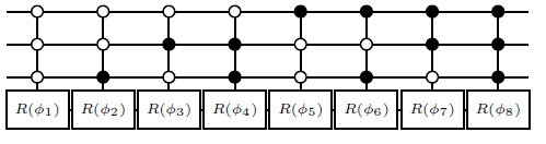
Recently Emmar2 , we have described a universal programmable circuit design which can be used to simulate the action of the matrix in Eq.(1) by simply determining the gate angles from the matrix elements. The idea is to independently generate circuit equivalences for the rows of in separate block quantum operations; and then combine the blocks by using different states of ancillary control qubits. This is shown in Fig.1.
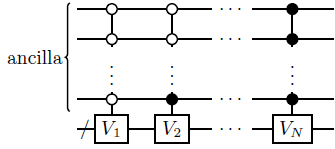
The circuit in Fig.1 can be represented by a block diagonal matrix with submatrices on the diagonal:
| (2) |
Here, each submatrix is to have the th row of the given matrix as their first rows in the following form: , where is the normalization constant. We use the sign “” for the elements that are insignificant in the overall scheme.
To use the matrix in place of the matrix in Eq.(1), we modify the input in Eq.(1) to a vector in a way that is populated with the elements of . Therefore, the expected output of can also be produced on some predetermined states in the outcome of . This is shown below:
| (3) |
where and are the normalization constants. In the above equation, the amplitudes {} on the states wherein the main qubits are zero are the same as the scaled expected outcomes of the application of to . The rest of the states in the output represented by “” is to be ignored. Therefore, the probability of success of the post-selection on the zero state of the main qubits, which is the success of the simulation, is given by . As an example, if , Eq.(3) becomes as follows:
| (4) |
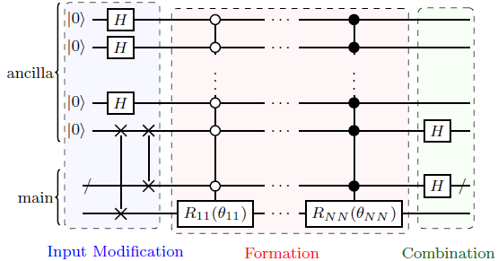
An instance circuit for this simulation technique is given in Fig.2 Emmar2 , which can simulate any given matrix based on Eq.(3). The separation of the main and the ancilla qubits in the circuit is largely artificial, since their role can be interchanged in the circuit. To ease the verification process, the circuit is divided into three blocks: Formation, Combination, and Input Modification as shown in the figure. The verification of this circuit is given in Appendix A.
In the phase estimation process, for simplicity, we swap the states of the first ancilla qubits with the main qubits at the end of the circuit, and use the following output instead of the one in Eq.(3):
| (5) |
where the first states are chosen to be important states. Measuring all the ancilla qubits in the computational basis and post-selecting for the result , one obtains in the remaining qubits in the state (as introduced in Eq. (1)). In this case, the success probability .
3 Finding Eigenvalues of Non-Unitary Matrices
The polar form of a complex eigenvalue, , belonging to a matrix, , can be written as:
| (6) |
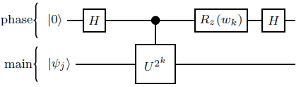
where is the phase and is the magnitude of the th eigenvalue. For unitary matrices, is equal to 1. Therefore, the well-known efficient quantum phase estimation algorithm (PEA) can be used to find the value of the phase, , and hence the eigenvalue . The circuit shown in Fig.3 is the iterative version of the phase estimation algorithm (IPEA) Miroslav ; Abrams ; Kitaev which can also be used to estimate the value of . In each iteration of IPEA, a bit of the -digit binary expansion of the phase is computed:
| (7) |
where is the total number of iterations, which determines the precision. is the binary value found from the th iteration of the IPEA using the th power of the matrix, .
However, for non-unitary matrices, the phase estimation algorithm alone is not enough. This is because two parameters, and , need to be found to compute the eigenvalue. In the following sections, we show that by using IPEA with the general circuit described in the previous section, parameters and can be determined, and hence eigenvalues of non-unitary matrices can also be found by the phase estimation algorithm without additional cost. Since our circuit design has a fixed size and scheme, the application of IPEA to the circuit design also has a fixed design. Therefore, we only need to set the angle values in each iteration of IPEA.
3.1 Estimation of
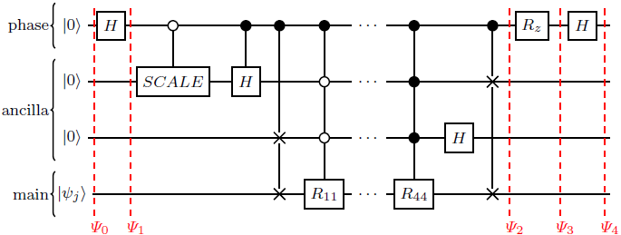
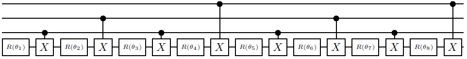
To use the general circuit design shown in Fig.2, within the IPEA framework, we need to determine the relationship between the chosen states and the phase qubit resulting in the measurement. As described in the previous section, the circuit scales the expected output of the chosen states by , which clearly originates from the Hadamard gates. Since there are Hadamard gates in the circuit, . In phase estimation, since all of the gates are controlled by the upper qubit, this scaling effect of exists only when the phase qubit is one. In order to have the same scaling when also the phase qubit is zero, we allow all Hadamard gates on the ancilla qubits except the one on the first ancilla qubit to operate without any control qubit. Instead of that controlled-Hadamard gate on the ancilla qubit, a scaling gate is used, which operates when the phase qubit is zero and has the following structure:
| (8) |
The resulting circuit is shown for two qubit systems in Fig.4. Here, we control all operations except the Hadamard gates on the ancilla qubits by the phase qubit. If the phase qubit is zero, for the input given in Eq.(1), this circuit produces the following on the remaining qubits:
| (9) |
where . Therefore, we can estimate the phase on the selected states, where the ancilla is zero in the output.
Considering the circuit in Fig.4, in one iteration of the phase estimation algorithm, the effect of the eigenvalue,
represented in polar form, can be observed in the evolution of the system as follows:
Fig.4, is:
| (10) |
where , , and represents the phase, ancilla and main qubits, respectively. is the eigenstate of the operator . After the first Hadamard gate on the phase qubit, the state becomes:
| (11) |
When the phase qubit is one, the application of the universal circuit generates the output on the chosen states. Since the Hadamard gates are not controlled, they are the only gates which operates when the phase qubit is zero. Therefore, after the application of the universal circuit with the gate (which scales the input state when the phase qubit is zero), we have the following:
| (12) |
where represents the universal circuit in Fig.2. From the eigenvalue equation, . On the chosen states, simulates . Hence, if we consider chosen states (the states where the ancilla is ), where is the normalization constant. Therefore, we have the following wave function describing the chosen states in the first iteration:
| (13) |
where the states which are not including are ignored. Application of the rotation gate around the z-axis on the phase qubit in the circuit guarantees that only one bit, in , of the phase is estimated in each iteration. Hence, after this gate, the term becomes :
| (14) |
After the last Hadamard applied to the phase qubit, the final state is as follows:
| (15) |
or more concisely:
| (16) |
Here, because of the system size, . For general case, is directly related to the size of the ancilla and is if there are qubits in the ancilla. Thus, the above equation can be represented in general form as follows:
| (17) |
Since is a bit value, it can be either 0 or 1. When , since , the above equation reduces to:
| (18) |
In the case, when , since , Eq.(17) becomes:
| (19) |
Since ; if , the probability to find the phase qubit in state is higher then the probability to find it in . If , then the probability to find the phase qubit in is higher. Thus, from the measurement on the phase qubit can be determined.
In each iteration of the phase estimation algorithm, a different bit of the phase is determined in this manner. For the th iteration of the phase estimation algorithm to determine the th digit of the phase, we see . Hence, for , the more we increase the power of or the accuracy, the more the amplitudes of the states, and , come closer. In this case, a single iteration of the PEA may repeat the protocol several times to collect enough statistics to determine the phase bit with high confidence. This is particularly important for later iterations, where, for , the probability of finding the phase qubit in or is exponentially (in the iteration index ) close.
3.2 Computing
As we have shown above, the output probability of the phase qubit when the ancilla is zero is determined by . We measure or with probability equal to . Hence, we get
| (20) |
Since and are known (for a matrix, the value of is due to two Hadamard gates in the circuit), can be determined from the statistics of the measurement. Therefore, the accuracy of the estimate value of can be further improved by using all iterations of the phase estimation algorithm: For the th iteration, as a general form, the following is obtained:
| (21) |
Taking the average of the estimates from different phase estimation iterations, the estimate of may become more accurate. Finally, by using values of and in Eq. (6), we can compute the eigenvalue of the non-unitary matrix.
4 Discussion
In the phase estimation algorithm, to be able to generate the matrix elements by using rotation gates around y- and z-axis, the absolute values of the elements should be less than one. One way to achieve this is to divide all the elements by the absolute value of the maximum element. Based on the norm and the eigenvalue relationship, this guarantees that the absolute value of the largest eigenvalue is less than the absolute row or column sums of the matrix which can be maximum (i.e. because the absolute value of the maximum is 1.). The eigenvalue is not required to be less than one. However, if the eigenvalue is greater than 1, this approach may require scaling in the very iteration of the algorithm since in the powers there is a possibility the elements may become greater than one again. Another approach to scale the elements is to use the 1-norm or the infinity-norm of the matrix, which are easy to compute. Scaling the matrix by the norm makes the eigenvalue less than 1, and so in the power of the matrix the elements goes to zero. Hence, the scaling is only done at the beginning. Therefore, in the th iteration of the phase estimation algorithm, we have , where is the scaling used at the beginning. Hence, if , without any scaling, the more we increase the power of or the accuracy, the more the amplitudes of the states, and , come closer. For , after a few iterations, it becomes infeasible to distinguish whether the phase qubit is 0 or 1. Scaling the powers of which generates the eigenvalue can be used to remedy this problem.
The accuracy for determining the value of , requires to determine the terms and in the probabilities for finding the phase qubit in or from the statistics on the measurements. The accuracy of in these statics differs based on the measurement protocol, the quantum state, the underlying quantum machine, and even the amount of the entanglement Usami2003 ; Bogdanov2011 .
4.1 Algorithmic Complexity
The complexity of one-iteration of the phase estimation algorithm is mainly dominated by the complexity of implementing the given operator. There is also need to obtain the state tomography of the phase qubit in order to determine the absolute value of the eigenvalue which differs based on the underlying quantum machine used for the phase estimation algorithm.
It is known that the complexity of implementing an operator on quantum computer requires number of one and two qubit operations Chuang . In addition, more efficient circuits are possible for the sparse matrices. The general circuit described in Fig.2 also obeys these complexity behavior (see ref.Emmar2 for the detailed complexity analysis of the circuit.). In the circuit, there is a quantum network composed of rotation gates uniformly controlled by the first qubits. The decomposition of this network requires number of CNOT and single rotation operations, which is explained in Appendix B. Therefore, the circuit in total requires CNOT, single rotation, Hadamard, and SWAP gates Emmar2 . Hence, the total complexity is . Also note that for zero elements, there is no need to use rotation gates. Thus, for the sparse matrices, the number of operations can be reduced Emmar2 .
Since the complexity of an iteration of the phase estimation algorithm is dominated by the complexity of the implementing the given operator, each iteration of the algorithm requires operations. Then for number of iterations, we get as the complexity.
When the powers of the matrix cannot be efficiently computed, the complexity of computing the power of matrix on classical computers should also be considered. The power of a matrix can be found by using the successive squaring method which requires only one matrix multiplication. Then the total complexity becomes the combination of these two:
| (22) |
where is the number of iterations, and is the complexity of matrix multiplication. Note that even if the powers of the matrix needs to be computed, this is still at least as efficient as the classical algorithms which requires in general time for finding an eigenvalue Golub . Also, note that the algorithmic complexity in Eq.(22) does not include the complexities of measuring and determining the value of . These are dependent on the measurement protocol, the quantum state, and the underlying quantum machine. In addition, the total number of iterations may be large in cases where, for , the probability of finding the phase qubit in or states gets exponentially (in the iteration index ) close, since a single iteration of the PEA may require repeating the protocol several times to collect enough statistics to determine the phase bit with high confidence.
In comparison to the work done by Wang et al. Hefeng-MPEA , the success probability decreases exponentially in both algorithms described in this paper and their paper. However, in our case by scaling the matrix elements in every iteration of the algorithm, the probability can be increased. Furthermore, here, one can finds the angle values for the rotation gates very easily (see Appendix B.1) to implement the given operator. However, in their method, one needs to find subsystems and and their interaction in order to implement the given : . In terms of quantum complexity, since their method is based on the non-unitary successive projective measurements on which cannot be implemented deterministically, the complexity is exponentially gets larger Hefeng-MPEA . On the other hand, in their case finding the powers of the given operator is easier, however, when the size of the subsystem is large, the complexity is dominated by the complexity of the measurements.
5 Application to Non-Hermitian Quantum Systems
Some problems can be extremely hard or even impossible to solve within the framework of the standard formalism of quantum mechanics where the observable properties of the dynamic nature are real and associated with the eigenvalues of Hermitian operators. Most extensions of the standard Hermitian formalism of quantum mechanics are equivalent to use a non-Hermitian operator instead of a Hermitian one. Resonance phenomena, where the particles are temporarily trapped by the potential, can be explored within the non-Hermitian quantum mechanics. In the non-Hermitian quantum mechanics, the lifetime of the resonant states are proportionally dependent on the behavior of the imaginary part of the eigenvalue Pablo ; Moiseyev2011 . Suppose we have the non-unitary operator for a non-Hermitian Hamiltonian with energy eigenstates and corresponding energy eigenvalues , i.e., . Since is an eigenvalue of ; if and are set to , then is the eigenvalue of . Therefore, a non-unitary transformation has eigenvectors , , …, , with corresponding eigenvalues . As shown in Sec.3, the eigenvalue of the matrix can be estimated. This also allows us to determine the corresponding eigenvalue of the Hamiltonian from . Note that in our phase estimation procedure, since the matrix elements are directly used in the circuit, one can also directly use the Hamiltonian matrix, , instead of .
5.1 Example
As an example, we consider the following radial Hamiltonian Pablo :
| (23) |
where and are free potential parameters ( is the depth of the potential in the potential graph. is related to the width of the potential barrier.) The potential term, , in the above Hamiltonian exhibits predissociation resonances which are quasibound states associated with the complex part of the eigenvalues Pablo . For the illustration purpose, using only two basis functions (the orthonormalized eigenfunctions of the harmonic oscillator, where mass equals one and the frequency equals ) and setting and ; the Hamiltonian matrix is found as 111This matrix is given by Pablo Serra, private communication, 2012. Pablo :
| (24) |
which has the eigenvector:
| (25) |
and the ground state eigenenergy . Since the above Hamiltonian matrix is non-Hermitian, the time evolution operator found from is non-unitary, which is found as:
| (26) |
with eigenvalue . We have used the phase estimation method described above to simulate this non-unitary operator and determine the complex eigenvalues of . In the simulation, since the absolute values of the matrix elements of are greater than 1, we scale the elements by the 1-norm of the matrix. This makes the matrix elements of go to zero in the limit. We use 11 iterations in the phase estimation algorithm. After the 11th iteration, the probability difference between seeing the phase qubit 0 or 1 becomes almost equal.
Therefore, from the simulation output, we find the eigenvalue of as , and so the eigenvalue of as , which gives an error in the order of . This comes from computer round-off errors and the limited available powers of (when the power of goes to zero, we can no longer distinguish between and on the phase qubit; the probabilities becomes the same). The simulation details are given in Appendix B.
6 Conclusion
We have presented a general scheme for the execution of the phase estimation algorithm for non-unitary matrices. Since the circuit design used for non-unitary matrices is a general programmable circuit, the circuit for the phase estimation algorithm is also universal: It can be used for any type of matrix to compute its eigenvalues. We have shown that the complex eigenvalues of non-Hermitian quantum systems can be found by using this method. As an example we have shown how to explore the resonance states of a model Hamiltonian.
7 Acknowledgement
We thank Pablo Serra for providing the Hamiltonian matrix used as an example in this paper. We also thank the two anonymous referees for their help in improving the clarity of this paper. This work is supported by the NSF Centers for Chemical Innovation: Quantum Information for Quantum Chemistry, CHE-1037992.
Appendix A Verification of the Circuit in Fig.2
The circuit is divided in three blocks: Formation, Combination, and Input Modification as shown in the figure. In the Input Modification block, the initial input is modified to . Then, the matrix is constructed in the Formation and Combination blocks.
A.0.1 Formation Block:
The second block in Fig.2 is called Formation Block which consists of uniformly controlled rotation gates for each element of . For the matrix element , assumed to be real, the rotation gate is defined as follows:
| (27) |
where is determined from the value of the element in accordance with the equality to get the following:
| (28) |
Based on the linear indices of the elements (row-wise), s are controlled by the different states of qubits: e.g., is the second element in the matrix and has a linear index of . Hence, the control of is set accordingly so that this gate operates when the first qubits in state. Combination of these controlled rotation gates forms a network as the second block in Fig.2. This block has the following matrix representation in the computational basis:
| (29) |
Here, we have used rotations around the y-axis since the matrix elements are assumed to be real. However, for the complex elements of , a product of and gates is needed for each . For instance, if , is created by , and is by .
A.0.2 Combination Block:
For a system of qubits, the third block in Fig.2 is defined as the application of the Hadamard gates to th, th, …, th, and th qubits from the top of the circuit: i.e. , where and are the Hadamard and identity matrices, respectively. The matrix representation of this block is as follows:
| (30) |
Note that also has negative elements, however, they are not located in the first row. Therefore, they shall not affect the predetermined states. The application of the above matrix to the matrix defined in Eq.(29) forms the matrix defined in Eq.(3) where the same row elements of are located on the leading rows of each ( represents the row index of ):
| (31) |
Since the negative elements are not in the first row of , the resulting leading rows are not affected by these elements. The elements represented by the symbol “” are disregarded by modifying the input to the circuit in the modification block explained below.
A.0.3 Input Modification Block:
The initial input to the circuit in Fig.2 is defined as where is the input to the ancilla qubits. The first block in Fig.2 consists of the Hadamard gates on the first qubits and sequential swap operations between the th and the remaining last qubits (We apply swap operations between the ancilla th qubit and the main qubits: First we swap the th qubit with the th, then the th with the th, then the th with the th, and so on. Finally we swap the th with the th). This block modifies the input in a way that in the application of to the input, the output is not affected by the elements represented by “” between and . Hence, the application of this block to the initial input transforms to in Eq.(3):
| (32) |
where is a normalization constant.
Consequently, the circuit in Fig.2 describes the operation which simulates any matrix , having elements less than or equal to 1, on the following normalized set of states: , , , where represents the ancilla qubits. This is shown in Eq.(3).
For illustration purposes, we also present the full forms of the operators for the formation, combination and input modification blocks and the output vector for the simulation of the following arbitrary matrix Emmar2 :
| (33) |
The full form of the matrix for the formation block is as follows:
| (34) |
The combination matrix and the matrix for the input modification are defined as:
| (35) |
For the initial input , we find the following final state:
| (36) |
Clearly the normalized states and simulate the original given system.
Appendix B Simulation Details
B.1 The decomposition of a multi controlled network
The circuit in Fig.2 includes a network of rotation gates in the formation block which dominates the complexity of the circuit. The uniformly controlled networks such as the one in Fig.5a controlled by qubits can be decomposed in terms of CNOT gates and single rotation gatesMottonen . For instance, the circuit as illustrated for in Fig.5a can be decomposed as in Fig.5b.
The angle values in the decomposed circuit are solutions of the system of the linear equation :
| (37) |
where is the number of control qubits in the network, and the entries of are defined as:
| (38) |
in which the power term is found by taking the dot product of the standard binary code of the index , , and the binary representation of th Gray coded integer, . Since is a column permuted version of the Hadamard matrix, we see that is unitary. Thus, , and the new angle values in the decomposed circuit are results of the matrix vector multiplicationMottonen :
| (39) |
B.2 Simulation Details for the Example System
In Fig.4, we have a multi controlled network composed of 4 gates. This network basically comes from the Formation step of the circuit design method, which has been represented in matrix form as in Eq.(29). Since the elements of are complex, we need to have rotations around the axis and the axis. Hence, the above matrix is the product of two matrices for rotation around the z-axis, and for rotations around the y-axis: :
| (40) |
To complete this network to a whole uniformly controlled network, we assume that the initial four other gates are identity. Hence, the final decomposition for matrix, the decomposed circuit includes: 4 Hadamard gates, 16 CNOT and 16 single gates (8 CNOTs and 8 gates for the ; and 8 CNOTs and 8 gates for the ), and 2 swaps.
The parameters for the last iteration (The operator is .) of the phase estimation algorithm is shown below, where after scaling the elements of by the matrix norm (maximum of the absolute sums of the columns), we find the angle values for and gates:
| Matrix Elements | Scaled Elements | Angles for s | Angles for s |
|---|---|---|---|
| 0.2588 + 1.1214i | 0.1469 + 0.6364i | 1.0521 | -0.9634 |
| -0.4569 - 0.1109i | -0.2593 - 0.0629i | 0.0278 | 0.1837 |
| -0.4569 - 0.1109i | -0.2593 - 0.0629i | -0.2486 | 1.9401 |
| 1.0594 + 0.7394i | 0.6012 + 0.4196i | 0.0278 | 0.1837 |
| -0.0278 | -0.1837 | ||
| 0.2486 | -1.9401 | ||
| -0.0278 | -0.1837 | ||
| -1.0521 | 0.9634 |
The angle value for the gate on the first qubit is -2.51572849. The output of the phase estimation algorithm on the chosen states and the normalized probability of the phase qubit are shown below.
| States | Probabilities on the Chosen States | Normalized Probabilities of the phase qubit |
|---|---|---|
| 0 | 0.0002 | 0.0058 |
| 1 | 0.001 | 0.9942 |
| 2 | 0.0393 | |
| 3 | 0.1765 |
The bit values of the phase is found as which corresponds to 0.9004. The absolute value of the eigenvalue is found from the ratio of the probability values of the phase qubit:
| (41) |
From the above, we find . The eigenvalue of is found as . The eigenvalue of the Hamitlonian matrix is found from which is .
References
- (1) A.W. Harrow, A. Hassidim, S. Lloyd, Phys. Rev. Lett. 103, 150502 (2009). DOI 10.1103/PhysRevLett.103.150502
- (2) Y. Cao, A. Daskin, S. Frankel, S. Kais, Molecular Physics 110(15-16), 1675 (2012). DOI 10.1080/00268976.2012.668289
- (3) D. Deutsch, Proceedings of the Royal Society of London. A. Mathematical and Physical Sciences 400(1818), 97 (1985). DOI 10.1098/rspa.1985.0070
- (4) C.H. Bennett, E. Bernstein, G. Brassard, U. Vazirani, SIAM J. Comput. 26(5), 1510 (1997). DOI 10.1137/S0097539796300933
- (5) M.A. Martin-Delgado, Sci. Rep. 2(302) (2012)
- (6) D.S. Abrams, S. Lloyd, Phys. Rev. Lett. 83(24), 5162 (1999). DOI 10.1103/PhysRevLett.83.5162
- (7) A. Papageorgiou, C. Zhang, Quantum Information Processing 11(2), 541 (2012). DOI 10.1007/s11128-011-0263-9
- (8) D. Finkelstein, In Gudehus, T., Kaiser, G., Perl- mutter, A. (eds.) Coral Gables Conference on Fundamental Interactions at High Energy. Center of Theoretical Studies. Gordon and Breach, New York (1969)
- (9) R. Feynman, International Journal of Theoretical Physics 21, 467 (1982). 10.1007/BF02650179
- (10) B.C. Sanders, Appl. Math. Inf. Sci 3(2), 117 (2009)
- (11) S. Raeisi, N. Wiebe, B.C. Sanders, New Journal of Physics 14(10), 103017 (2012)
- (12) I. Kassal, S.P. Jordan, P.J. Love, M. Mohseni, A. Aspuru-Guzik, Proceedings of the National Academy of Sciences 105(48), 18681 (2008)
- (13) D.W. Berry, G. Ahokas, R. Cleve, B.C. Sanders, Communications in Mathematical Physics 270(2), 359 (2007)
- (14) D. Lidar, H. Wang, Phys. Rev. E 59, 2429 (1999)
- (15) K.L. Brown, W.J. Munro, V.M. Kendon, Entropy 12 (2010)
- (16) D. Lu, B. Xu, N. Xu, Z. Li, H. Chen, X. Peng, R. Xu, J. Du, Phys. Chem. Chem. Phys. 14, 9411 (2012). DOI 10.1039/C2CP23700H
- (17) I. Kassal, J.D. Whitfield, A. Perdomo-Ortiz, M.H. Yung, A. Aspuru-Guzik, Annual Review of Physical Chemistry 62(1), 185 (2011). DOI 10.1146/annurev-physchem-032210-103512. PMID: 21166541
- (18) K.C. Young, M. Sarovar, J. Aytac, C. Herdman, K.B. Whaley, Journal of Physics B: Atomic, Molecular and Optical Physics 45(15), 154012 (2012)
- (19) A. Kitaev, Electronic Colloquium on Computational Complexity (ECCC) 3(3) (1996)
- (20) A. Aspuru-Guzik, A. Dutoi, P. Love, M. Head-Gordon, Science 309, 1704 (2005)
- (21) H. Wang, S. Kais, A. Aspuru-Guzik, M. Hoffmann, Phys.Chem.Chem.Phys. 10, 5388 (2008)
- (22) L. Veis, J. Pittner, J. Chem. Phys. 133, 194106 (2010)
- (23) A. Daskin, S. Kais, J. Chem. Phys. 134(14), 144112 (2011). DOI 10.1063/1.3575402
- (24) B.P. Lanyon, J.D. Whitfield, G.G. Gillett, M.E. Goggin, M.P. Almeida, I. Kassal, J.D. Biamonte, M. Mohseni, B.J. Powell, M. Barbieri, A. Aspuru-Guzik, A.G. White, Nature Chemistry 2(2), 106 (2010). DOI 10.1038/nchem.483
- (25) A. Aspuru-Guzik, P. Walther, Nat Phys 8(4), 285 (2012). DOI 10.1038/nphys2253
- (26) J. Du, N. Xu, X. Peng, P. Wang, S. Wu, D. Lu, Phys. Rev. Lett. 104, 030502 (2010). DOI 10.1103/PhysRevLett.104.030502
- (27) N. Moiseyev, Non-Hermitian quantum mechanics (Cambridge University Press, 2011)
- (28) H. Terashima, M. Ueda, International Journal of Quantum Information 03(04), 633 (2005). DOI 10.1142/S0219749905001456
- (29) H. Wang, L. Wu, Y. Liu, F. Nori, Phys. Rev. A 82, 062303 (2010). DOI 10.1103/PhysRevA.82.062303
- (30) H. Terashima, Phys. Rev. A 85, 022124 (2012). DOI 10.1103/PhysRevA.85.022124
- (31) A. Daskin, A. Grama, G. Kollias, S. Kais, The Journal of Chemical Physics 137(23), 234112 (2012). DOI 10.1063/1.4772185
- (32) M. Dobšíček, G. Johansson, V. Shumeiko, G. Wendin, Phys. Rev. A 76(3), 030306 (2007)
- (33) K. Usami, Y. Nambu, Y. Tsuda, K. Matsumoto, K. Nakamura, Phys. Rev. A 68, 022314 (2003). DOI 10.1103/PhysRevA.68.022314. URL http://link.aps.org/doi/10.1103/PhysRevA.68.022314
- (34) Y.I. Bogdanov, G. Brida, M. Genovese, S.P. Kulik, E.V. Moreva, A.P. Shurupov, Phys. Rev. Lett. 105, 010404 (2010). DOI 10.1103/PhysRevLett.105.010404. URL http://link.aps.org/doi/10.1103/PhysRevLett.105.010404
- (35) M.A. Nielsen, I.L. Chuang, Quantum Computation and Quantum Information (Cambridge University Press, 2000)
- (36) G.H. Golub, C.F. Van Loan, Matrix computations (3rd ed.) (Johns Hopkins University Press, Baltimore, MD, USA, 1996)
- (37) P. Serra, S. Kais, N. Moiseyev, Phys. Rev. A 64, 062502 (2001). DOI 10.1103/PhysRevA.64.062502
- (38) M. Möttönen, J.J. Vartiainen, V. Bergholm, M.M. Salomaa, Phys. Rev. Lett. 93, 130502 (2004). DOI 10.1103/PhysRevLett.93.130502