Current Sheet Statistics in Three-Dimensional Simulations of Coronal Heating

Abstract

In a recent numerical study [Ng et al., Astrophys. J. 747, 109, 2012], with a three-dimensional model of coronal heating using reduced magnetohydrodynamics (RMHD), we have obtained scaling results of heating rate versus Lundquist number based on a series of runs in which random photospheric motions are imposed for hundreds to thousands of Alfvén time in order to obtain converged statistical values. The heating rate found in these simulations saturate to a level that is independent of the Lundquist number. This scaling result was also supported by an analysis with the assumption of the Sweet-Parker scaling of the current sheets, as well as how the width, length and number of current sheets scale with Lundquist number. In order to test these assumptions, we have implemented an automated routine to analyze thousands of current sheets in these simulations and return statistical scalings for these quantities. It is found that the Sweet-Parker scaling is justified. However, some discrepancies are also found and require further study.

¹Space Science Center, University of New Hampshire, Durham, NH 03824

²Geophysical Institute, University of Alaska Fairbanks, Fairbanks, AK 99775

³Princeton Plasma Physics Laboratory, Princeton, NJ 08543

1 Introduction

Within the framework of the parker model of coronal heating (Parker 1972), a recent analysis (Ng & Bhattacharjee 2008) in two dimensions (2D) demonstrated that when coherence times ($\tau_{c}$) of the imposed photospheric turbulence are much smaller than characteristic resistive time-scales ($\tau_{R}$), the Ohmic dissipation scales independently of resistivity. While their initial 2D RMHD treatment precluded non-linear effects such as instabilities and/or magnetic reconnection, they further invoked a simple analytical argument demonstrated that even with these non-linear effects, which would limit the growth of $B_{\perp}$ (the component of the magnetic field perpendicular to a guide field $B_{z}$), the insensitivity to resistivity is still true for small enough $\tau_{c}$. This latter hypothesis was subsequently confirmed (Ng et al. 2012) by means of 3D RMHD simulations of the Parker model which spanned three orders of magnitude in Lundquist number.

The scalings derived in these studies depend critically on the assumption that the classical 2D steady-state Sweet-Parker scaling for magnetic reconnection holds in 3D simulations where extended current sheets form due to random boundary driving. In order to empirically substantiate this assumption, and to look into the nature of stochastically driven magentofluids in more details, we have carried out a systematic analysis of current sheets formed in our simulations.

We report here a simple algorithm to identify and characterize individual current layers. Statistics are accumulated for current sheet parameters. In Section 2, we develop and review the motivating analysis. Section 3 describes our simple algorithm. Section 4 reports our findings and outstanding issues with our analysis.

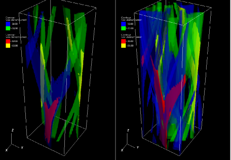
Figure 1.: 3D iso-surfaces of current sheets.

2 Coronal Heating Scaling Analysis

In the parker model, a solar coronal loop is treated as a straight ideal plasma column, bounded by two perfectly conducting end-plates representing the photosphere. Initially, there is a uniform magnetic field along the $z$ direction. The footpoints of the magnetic field on the photosphere are frozen (line-tied), subjected to slow, random motion $\phi(z=0,t)$ and $\phi(z=L,t)$ that deform the magnetic field.

The footpoint motion is assumed to take place on a time scale much longer than the characteristic time for Alfvén wave propagation between $z=0$ and $z=L$, so that the plasma can be assumed to be in quasi static equilibrium nearly everywhere, if such equilibrium exists, during this random evolution. For a given equilibrium, a footpoint mapping can be defined by following field lines from one plate to the other. Since the plasma is assumed to obey the ideal MHD equations, the magnetic field lines are frozen in the plasma and cannot be broken during the twisting process. Therefore, the footpoint mapping must be continuous for smooth footpoint motion. Parker (1972) claims that if a sequence of random footpoint motion renders the mapping sufficiently complicated, there will be no smooth equilibrium for the plasma to relax to, and tangential discontinuities (or current sheets) of the magnetic field must develop. Parker treated the corona as ideal given that the Lundquist number of the corona is estimated to be of the order of $10^{13}$. Being of ultimately finite resistivity however, it is suggested that ohmic dissipation in these current sheets can significantly account for heating coronal plasma.

Resolving current sheets at realistic values of Lundquist numbers remains well beyond the reach of current computational capabilities with direct numerical MHD simulations. Useful scaling studies, however, have been carried out by numerous investigators (cf. Ng et al. 2012 for references). Our current numerical study is motivated by scaling analysis for coronal heating that, unlike previous derivations of the coronal heating rate, considers the effects of random footpoint motion. We quickly summarize the main arguments here (cf. Ng & Bhattacharjee 2008 and Ng et al. 2012 for details).

In well resolved direct time-dependent, 3D RMHD numerical simulations of the Parker model, on average, at any given time, there will be $N$ current sheets with characteristic width ($\lambda$) and length ($\Delta$), which span the length of the simulation box ($L$). The characteristic time over which energy is built-up by random photospheric motions and subsequently released is $\tau_{E}$, and therfore the average heating rate due to ohmic dissipation can be written as:

$$\bar{W}\sim\eta N\Delta L\frac{\bar{B}^{2}_{\perp}}{\lambda}\sim\frac{\bar{B}^{2}_{\perp}LL^{2}_{\perp}}{\tau_{E}},$$ (1)

where $\eta$ is the plasma resistivity and $\bar{B}^{2}_{\perp}$ is the average magnetic field. An expression for the average perpendicular magnetic field can be estimated considering that over a duration of ${\tau_{E}}$, photospheric footpoint motions of average velocity $v_{p}$, if assumed constant, would deform the guide field $B_{z}$ and produce $\bar{B}_{\perp}$ up to a level of

$$\bar{B}_{\perp}\sim B_{z}\frac{v_{p}\tau_{E}}{L}\sim\left[\left(\frac{B_{z}v_{p}}{LN}\right)^{2}\frac{L^{4}_{\perp}}{w\eta}\right]^{1/3},$$ (2)

where, for the latter expression, we have solved for ${\tau_{E}}$ in Equation (1) using the Sweet-Parker current sheet scaling given by $\lambda/\Delta\sim S_{\perp}^{1/2}$. We define the Lundquist number here as $S_{\perp}\equiv wB_{\perp}/\eta$, with $w=v_{p}\tau_{c}$ being the typical transverse length scale of the magnetic field. Together, Equations (1) and (2) yield the following expression for the average heating rate:

$$\bar{W}\sim\left(\frac{L^{10}_{\perp}B_{z}^{5}v_{p}^{5}}{L^{2}N^{2}w\eta}\right)^{1/3}.$$ (3)

Evidently, when one extrapolates to the collisionless coronal limit, the heating rate predicted here becomes un-physically large. If we rewrite however the expression for the perpendicular magnetic field production considering the turbulent motions in the photosphere to have a random walk nature: $\bar{B}_{\perp}\sim B_{z}v_{p}(\tau_{c}\tau_{E})^{1/2}/L$, an average heating rate can be estimated as:

$$\bar{W}\sim\frac{L^{2}_{\perp}}{L}B_{z}^{2}v_{p}^{2}\tau_{c}.$$ (4)

Equation (4) is manifestly independent of resistivity, and holds when $\tau_{c}<\tau_{E}$, i.e. when the effects of random motion become important. In Ng et al. (2012) we have studied the transition of the heating rate into this regime with numerical simulations spanning three orders of magnitude. In the regime where $\tau_{c}>\tau_{E}$, we find good agreement with a previous study (Longcope & Sudan 1994), with the heating rate scales as $\bar{W}\propto{\eta^{1/3}}$. While in the high Lundquist number regime where $\tau_{c}<\tau_{E}$, we recover an $\eta$ independent behavior. The reader is referred to Ng et al. (2012) for an in depth discussion of these results. Here we focus on an ancillary study that addresses two key assumptions made in arriving at the scaling relations here: $(1)$ The number of current sheets $N$ is essentially independent of Lundquist number; and $(2)$ The Sweet-Parker scaling, which derives from a 2D quasi-steady theory, is applicable more generally in our 3D line-tied model with driving applied at the boundaries. We assess these two assumptions by means of a straightforward algorithm.

3 Current Sheet Identification and Fitting

Our MHD simulations employ the reduced MHD equations and are solved using a standard algorithm (described in Ng et al. 2012, and have been recently accelerated via GPUs with NVidia CUDA as shown in Lin et al. 2012). Our current goal is to identify and characterize individual current layers forming in time-dependent 3D simulations of a coronal loop driven at the line-tied boundaries. Figure 1 shows iso-surfaces of current density for a snapshot of one of our simulation runs (with $S_{\perp}\sim 5000$). As a starting point, we examine only the 2D cross section at $z=L/2$ of our simulation domain.

This task is formidable for the following reasons: $(1)$ Given the stochastic nature of the imposed photospheric boundary driving, current sheet orientations are random. $(2)$ We are dealing with tens of thousands of individual instances of current sheets forming during steady state evolution of the Parker model, for which we have data cubes saved at a prescribed cadence. $(3)$ We use periodic boundary conditions in which current sheets often traverse the edges. $(4)$ In three dimensions, current sheets appear to branch out, so a structure appearing as a single current layer in one specific cross-section of the loop might appear as several in a different cross-section at a location further along the loop, possibly with different properties. Figure 1 attests to each of these issues.

Our approach consists of two steps. First, an ad-hoc thresholding algorithm identifies current sheet candidates by simply taking all pixels in $|J|$ above a pre-defined fraction of $|J|_{max}$ and testing for contiguity of the selected regions. This is done in two-dimensional cross-sections of the loop simulations, with the algorithm accounting for the periodic boundary conditions used by the pseudo-spectral RMHD scheme. By this we mean that a current sheet that appears at a border of the simulation box will appear at the other border (or at up to 4 edges if it appears at a corner), but will be identified only one occurrence. This feature is crucial, considering that we are automating this procedure to analyze tens of thousands of simulation cube samples and the likelihood of current sheets appearing at domain edges is quite high. Figure 2(a) shows a contour plot of current density for a cross-section of one of our simulations. Current sheet candidates identified by the routine are labeled by green bracketed numbers. The structures labeled $[1]$ and $[6]$, for example, appear at edges but are uniquely identified.

After current sheet candidates are identified they are morphologically examined by another automated algorithm, which performs least-square fitting with a bi-variate Gaussian. The automated algorithm is implemented using fitting and parameter constraining tools found in the Package for the Interactive Analysis of Line Emission (PINTofALE, Kashyap & Drake 2000).

Together, these two algorithms yield current sheet orientations with respect to the axes ($\theta$), number of current sheets present ($N$), local $J_{max}$, together with $\sigma_{small}$ and $\sigma_{large}$, which serve as proxies for current sheet width ($\lambda$) and current sheet length ($\Delta$), respectively. The three other panels in Figure 2 show one such fit for the current sheet labeled [9]. A surface plot shows $|J|$ in the region where current sheet [9] resides in plot (b). Plot(c) shows the bi-variate Gaussian fit and (d) shows the residual. The primary shortfalls of this approach can be summarized as follows: $(1)$ Many current sheets are not well approximated by bi-variate Gaussians. Profiles are often asymmetric, and the 2-D support of the current sheet structures is often bow-shaped rather than linear. $(2)$ Because we are taking only discrete samples in time (full data cubes are saved at a pre-determined cadence during simulations runs), the measurements will be biased towards current sheet structure that is most long-lived during the lifetime of the sheets. $(3)$ In the present analysis, the threshold for structure detection is set at $10\%$ of maximum $|J|$ (as measured in each time step), low enough so that most local maxima are included. Unfortunately, this renders the iterative search approach we take, while robust, quite computationally expensive. At higher resolutions, this becomes prohibitive, and requires re-sampling to lower resolution for reasonable run-times.

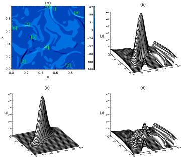
Figure 2.: Example of current sheet identification and fitting.

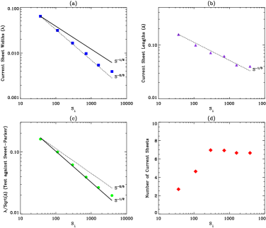
Figure 3.: Scaling of measured current sheet parameters with Lundquist number.

4 Summary of Results & Conclusions

Our current sheet identification and fitting routines have been applied to high resolution data set of Ng et al. (2012), producing a large sample of fits in the range of thousands to tens of thousands of current sheets per simulation run.

In Figure 3, we report weighted average quantities, where we use goodness-of-fit from the least square bi-variate Gaussian fitting as the weighting factor. Plots (a) and (b) show weighted average values for current sheet widths and lengths as a function of Lundquist number $S_{\perp}$. Plot (c) demonstrates good agreement with Sweet-Parker scaling. Plot (d) shows the number of current sheets averaged over all post-processed time slices. These results provide some empirical support for the assumptions we used for our scaling analysis. It is noted however that, even if the Sweet-Parker scaling of $\lambda/\Delta^{-1/2}\propto S_{\perp}^{-1/2}$ is recovered, both the current sheet width ($\lambda\propto S_{\perp}^{-2/3}$) and current sheet length ($\Delta\propto S_{\perp}^{-1/3}$) decrease with the increase of $S_{\perp}$ faster than the scalings ($\lambda\propto S_{\perp}^{-1/2}$, $\Delta\sim$ constant) assumed in both Ng et al. (2012) and Longcope & Sudan (1994).

A more detailed analysis of these current sheet fitting results, and an extension of this analysis to examine the 3D structure of current layers is now underway. Of particular interest here is how the spatial separation of dissipative events in these simulations can inform an analysis of flare energy distributions, which typically only consider temporal variations in event definition (cf. Buchlin et al. 2005; Ng & Lin 2012).

Acknowledgments

Computer time was provided by UNH (using the Zaphod cluster at the Institute for the Study of Earth, Oceans, and Space), and HPC resources from the Arctic Region Supercomputing Center, the DoD High Performance Computing Modernization Program. This research is supported in part by grants from NSF (AGS-0962477 and AGS-0962698) and NASA (NNX08BA71G, NNX09AJ86G, NNX06AC19G, and NNX10AC04G) and DOE (DE-FG0207ER46372), and by NSF through TeraGrid resources provided by NCSA under grant number TG-PHY100057 and through computational resources provided by NICS under grant UT-NTNL0092.

References

- Buchlin et al. (2005) Buchlin, E., Galtier, S., & Velli, M. 2005, Astron. & Astrophys., 436, 355
- Kashyap & Drake (2000) Kashyap, V., & Drake, J. J. 2000, Bulletin of the Astronomical Society of India, 28, 475
- Lin et al. (2012) Lin, L., Ng, C. S., & Bhattacharjee, A. 2012, ASP Conf. Series, 459, 222
- Longcope & Sudan (1994) Longcope, D. W., & Sudan, R. N. 1994, Astrophys. J., 437, 491
- Ng & Bhattacharjee (2008) Ng, C. S., & Bhattacharjee, A. 2008, Astrophys. J., 675, 899
- Ng & Lin (2012) Ng, C. S., & Lin, L. 2012, AIP Conf. Proc., 1500, 38
- Ng et al. (2012) Ng, C. S., Lin, L., & Bhattacharjee, A. 2012, Astrophys. J., 747, 109
- Parker (1972) Parker, E. N. 1972, Astrophys. J., 174, 499