Evolutionary dynamics of time-resolved social interactions

Abstract

Cooperation among unrelated individuals is frequently observed in social groups when their members combine efforts and resources to obtain a shared benefit that is unachievable by an individual alone. However, understanding why cooperation arises despite the natural tendency of individuals towards selfish behavior is still an open problem and represents one of the most fascinating challenges in evolutionary dynamics. Recently, the structural characterization of the networks in which social interactions take place has shed some light on the mechanisms by which cooperative behavior emerges and eventually overcomes the natural temptation to defect. In particular, it has been found that the heterogeneity in the number of social ties and the presence of tightly knit communities lead to a significant increase in cooperation as compared with the unstructured and homogeneous connection patterns considered in classical evolutionary dynamics. Here, we investigate the role of social-ties dynamics for the emergence of cooperation in a family of social dilemmas. Social interactions are in fact intrinsically dynamic, fluctuating, and intermittent over time, and they can be represented by time-varying networks. By considering two experimental data sets of human interactions with detailed time information, we show that the temporal dynamics of social ties has a dramatic impact on the evolution of cooperation: the dynamics of pairwise interactions favors selfish behavior.

I Introduction

The organizational principles driving the evolution and development of natural and social large-scale systems, including populations of bacteria, ant colonies, herds of predators, and human societies, rely on the cooperation of large populations of unrelated agents penni05 ; penni09 ; maynard95 . Even if cooperation seems to be a ubiquitous property of social systems, its spontaneous emergence is still a puzzle for scientists, since cooperative behaviors are constantly threatened by the natural tendency of individuals towards self-preservation and the never-ceasing competition among agents for resources and success. The preference for selfishness over cooperation is also due to the higher short-term benefits that a single (defector) agent obtains by taking advantage of the joint efforts of cooperating agents. Obviously, the imitation of such selfish (but rational) conduct drives the system towards a state in which the higher benefits associated with cooperation are no longer achievable, with dramatic consequences for the whole population. Consequently, the relevant question to address is why cooperative behavior is so common in nature and society, and what are the circumstances and the mechanisms that allow it to emerge and persist.

In recent decades, the study of the elementary mechanisms fostering the emergence of cooperation in populations subjected to evolutionary dynamics has attracted a lot of interest in ecology, biology, and social sciences nowak06 ; kollock98 . The problem has been tackled through the formulation of simple games that neglect the microscopic differences among distinct social and natural systems, thus providing a general framework for the analysis of evolutionary dynamics maynard73 ; maynard82 ; gintis09 . Most of the classical models studied within this framework made the simplifying assumption that social systems are characterized by homogeneous structures, in which the interaction probability is the same for any pair of agents and constant over time samuelson02 . However, the theory of complex networks has proven this assumption false for real systems, by revealing that most natural and social networks exhibit large heterogeneity and non–trivial interconnection topologies watts ; strogatz ; rev:albert ; rev:newman . It has also been shown that the structure of a network has dramatic effects on the dynamical processes taking place on it, so that complex networks analysis has become a fundamental tool in epidemiology, computer science, neuroscience, and social sciences rev:bocc ; rev:doro2 ; rev:castellano .

The study of evolutionary games on complex topologies has led to a new way out for cooperation to survive in some paradigmatic cases such as the Prisoner’s Dilemma pachprl ; pachpnas ; prl ; assenza or the Public Goods games pachnature ; chaosPGG ; percpggrev . In particular, it has been pointed out that the complex patterns of interactions among the agents found in real social networks, such as scale-free distributions of the number of contacts per individual or the presence of tightly-knit social groups, tend to favor the emergence and persistence of cooperation. This line of research, which brings together the tools and methods from the statistical mechanics of complex networks and the classical models of evolutionary game dynamics, has effectively became a new discipline, known as evolutionary graph theory szaborev ; jackson08 ; anxorev ; percrev ; grossrev .

Recently, the availability of longitudinal spatio-temporal information about human interactions and social relationships eaglepentland ; scott ; isella ; sthele_primary has revealed that social systems are not static objects at all: contacts among individuals are usually volatile and fluctuate over time cattuto ; saramaki , face-to-face interactions are bursty and intermittent barabasi2005 ; bianconi2 , and agents motion exhibits long spatio-temporal correlations gonzales ; szell ; sinatra . Consequently, static networks, constructed by aggregating in a single graph all the interactions observed among a group of individuals across a given period, can only be considered as simplified models of real networked systems. For this reason, time-varying graphs have been introduced recently as a more realistic framework to encode time-dependent relationships kossinets ; kostakos ; tang_distance ; holme_review ; tang_sw . In particular, a time-varying graph is an ordered sequence of graphs defined over a fixed number of nodes, where each graph in the sequence aggregates all the edges observed within a certain temporal interval. The introduction of time as a new dimension of the graph gives rise to a richer structure. Therefore, new metrics specifically designed to characterize the temporal properties of graph sequences have been proposed, and most of the classical metrics defined for static graphs have been extended to the time-varying case nicosia_chapter ; tang_sw ; pan_paths ; kovanen_motifs ; tang_centrality ; nicosia_components ; mucha10 . Recently, the study of dynamical processes taking place on time-evolving graphs has shown that temporal correlations and contact recurrence play a fundamental role in diverse settings such as random walks dynamics starnini_rw ; perra_walking ; ribeiro2013 , the spreading of information and diseases rocha_1 ; rocha_2 ; rocha_3 , and synchronization diazguilera .

Here we study how the level of cooperation is affected when one considers a more realistic picture, in which the interactions in a social system are represented by time-varying graphs instead of classical (static) ones. We consider a family of social dilemmas, including the Hawk-Dove, the Stag Hunt, and the Prisoner’s Dilemma games, played by agents connected through a time-evolving topology obtained from real traces of human interactions. We analyze the effect of temporal resolution and correlations on the emergence of cooperation in two paradigmatic data sets of human proximity, namely the MIT Reality Mining eaglepentland and the INFOCOM’06 scott co-location traces. We find that the level of cooperation achievable on time-varying graphs depends crucially on the interplay between the speed at which the network changes and the typical time scale at which agents update their strategy. In particular, cooperation is facilitated when agents keep playing the same strategy for longer intervals, while too frequent strategy updates tend to favor defectors. Our results also suggest that the presence of temporal correlations in the creation and maintenance of interactions hinders cooperation, so that synthetic time-varying networks in which link persistence is broken usually exhibit a considerably higher level of cooperation. Finally, we show that both the average size of the giant component and the weighted temporal clustering calculated across different consecutive time windows are indeed good predictors of the level of cooperation attainable on time-varying graphs.

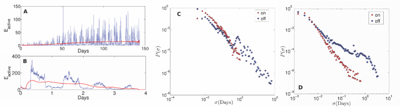
Figure 1: (Color online). Activity patterns of human interactions. The number $E_{\text{active}}$ of links in the graph at time $t$ is reported as a function of time for MIT Reality Mining (a) and INFOCOM’06 (b). Weekly and daily periodicities are visible. Red (light gray) lines display the moving averages, over a 1-month and a 1-day windows, respectively, revealing the non-stationarity of the sequences. Distributions of edge -active and -inactive periods (triangles and circles, respectively) for MIT Reality Mining (c) and INFOCOM’06 (d). The data were log-binned. The peak at $\sigma\sim 1$ for the inactive periods corresponds to 24 hours.

II Evolutionary Dynamics on Time-Varying Graphs

II.1 Evolutionary dynamics of social dilemmas

We focus on the emergence of cooperation in systems whose individuals face a social dilemma between two possible strategies: Cooperation ($C$) and Defection ($D$). A large class of social dilemmas can be formulated as in pachpnas via a two-parameter game described by the payoff matrix:

$$\bordermatrix{&C&D\cr C&R&S\cr D&T&P\cr}=\bordermatrix{&C&D\cr C&1&S\cr D&T&0\cr}\;,$$ (1)

where $R$, $S$, $T$, and $P$ represent the payoffs corresponding to the various possible encounters between two players. Namely, when the two players choose to cooperate, they both receive a payoff $R=1$ (for Reward), while if they both decide to defect they get $P=0$ (for Punishment). When a cooperator faces a defector it gets the payoff $S$ (for Sucker) while the defector gets $T$ (for Temptation). In this version of the game, the payoffs $S$ and $T$ are the only two free parameters, and their respective values induce an ordering of the four payoffs that determines the type of social dilemma. We have in fact three different scenarios. When $T>1$ and $S>0$, defecting against a cooperator provides the largest payoff, and this corresponds to the Hawk-Dove game. For $T<1$ and $S<0$, cooperating with a defector is the worst case, and we have the Stag Hunt game. Finally, for $T>1$ and $S<0$, when a defector plays with a cooperator, we have at the same time the largest (for the defector) and the smallest (for the cooperator) payoffs, and the game corresponds to the Prisoner’s Dilemma. In this work, we consider the three types of games by exploring the parameter regions $T\in[0,2]$ and $S\in[-1,1]$.

In real social systems, each individual has more than one social contact at the same time. This situation is usually represented anxorev by associating each player $i,~{}i=1,2,\ldots,N$ to a node of a static network, with adjacency matrix $A=\{a_{ij}\}$, whose edges indicate pairs of individuals playing the game. In this framework, a player $i$ selects a strategy, plays a number of games equal to the number of her neighbors, $k_{i}=\sum_{j}a_{ij}$, and accumulates the payoffs associated with each of these interactions. Obviously, the outcome of playing with a neighbor depends on the strategies selected by both players, according to the payoff matrix in Eq. (1). When all the individuals have played with all their neighbors in the network, they update their strategies as a result of an evolutionary process, i.e., according to the total collected payoff. Namely, each individual $i$ compares her cumulated payoff, $p_{i}$, with that of one of her neighbors, say $j$, chosen at random. The probability $P_{i\rightarrow j}$ that agent $i$ adopts the strategy of her neighbor $j$ increases with the difference $(p_{j}-p_{i})$. Here we adopt the so-called Fermi update fermi1 ; fermi2 in which the probability that agent $i$ copies the strategy of the randomly chosen neighbor $j$ reads:

$$P_{i\rightarrow j}=\dfrac{1}{1+e^{-\beta(p_{j}-p_{i})}}\;,$$ (2)

where $\beta$ is a parameter controlling the smoothness of the transition from $P_{i\rightarrow j}=0$ for small values of $(p_{j}-p_{i})$, to $P_{i\rightarrow j}=1$ for large values of $(p_{j}-p_{i})$. Notice that for $\beta\ll 1$ we obtain $P_{i\rightarrow j}\simeq 0.5$ regardless of the value of $(p_{j}-p_{i})$, which effectively corresponds to a random strategy update. On the other hand, when $\beta\gg 1$ then $P_{i\rightarrow j}\simeq\Theta(p_{j}-p_{i})$, where $\Theta(x)$ is the Heaviside step function. Here we adopt $\beta=1$, although we have checked that the results are qualitatively similar for a broad range of values of $\beta$.

The games defined by the payoff matrix in Eq. (1) and the use of a payoff-based strategy update rule have been thoroughly investigated in static networks with different topologies. The main result is that, when the network is fixed and agent strategies are allowed to evolve over time, the level of cooperation increases with the heterogeneity of the degree distribution of the network, with scale-free networks being the most paradigmatic promoters of cooperation pachprl ; pachpnas ; prl . However, in most cases human contacts and social interactions are intrinsically dynamic and varying in time, a feature that has profound consequences on any process taking place over a social network. We explore here the role of time on the emergence of cooperation in time-varying networks.

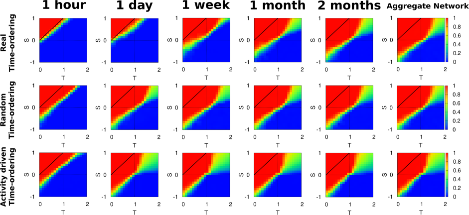
Figure 2: (Color online). Cooperation diagrams for the MIT Reality Mining data set. Fraction of cooperators at the equilibrium as a function of the temptation to defect (T) and of the sucker’s score (S) for different values of the interval $\Delta t$ between two successive strategy updates. From left to right, the diagrams correspond to $\Delta t$ equal to 1 hour, 1 day, 1 week, 1 month, 2 months, and to the entire observation period $M\tau\simeq 5$ months. The diagrams in the top row correspond to time-varying graphs with original time ordering, those in the middle row are obtained for the same values of $\Delta t$ but on randomized time-varying graphs, while the bottom row reports the results obtained on synthetic networks constructed through the activity-driven model. The results are averaged over 50 different realizations. Red (light gray) corresponds to $100\%$ of cooperators while blue (dark gray) indicates $100\%$ defectors. By focusing on a row, and proceeding from left to right, it is evident that there exists a value of the update interval $\Delta t$ above which the differences in the cooperation diagram are mostly limited to the region which separates the two phases (100% defectors and 100% cooperators), while the rest of the phase diagram is already indistinguishable from that corresponding to the aggregate graph. Moreover, for a fixed value of $\Delta t$, we observe that randomized and synthetic sequences are associated with an overall larger level of cooperation than the original ones. See Fig. 8 for additional details.

II.2 Temporal patterns of social interactions

In the following, we consider two data sets describing the temporal patterns of human interactions at two different time scales. The first data set has been collected during the MIT Reality Mining experiment eaglepentland , and it includes information about the spatial proximity of a group of students, staff, and faculty members at the Massachusetts Institute of Technology, over a period of six months. The resulting time-dependent network has $N=100$ nodes and consists of a time-ordered sequence $\{G_{1},G_{2},\ldots,G_{M}\}$ of $M=41291$ graphs (snapshots), each graph representing proximity interactions during a time interval of $\tau=5$ minutes. Remember that each graph $G_{m}$ ($m=1,\ldots,M$) accounts for all the instantaneous interactions taking place in the temporal interval $[(m-1)\tau,m\tau]$. The second data set describes co-location patterns, over a period of four days, among the participants of the INFOCOM’06 conference scott . In this case, the resulting time-dependent network has $N=78$ nodes, and it contains a sequence of $M=2880$ graphs obtained by registering users co-location every $\tau=2$ minutes. Additional details about the two data sets are reported in Appendix A.

The frequency of social contacts is illustrated in Fig. 1 [panels (a) and (b)], where we report the number of active links at time $t$, $E_{\text{active}}$, as a function of time. In the MIT Reality Mining data set, social activity exhibits daily and weekly periodicities, respectively due to home–work and working days-weekends cycles. In addition to these rhythms, we notice a non-stationary behavior which is clearly visible when we plot the activity averaged over a 1-month moving window [red line in panel (a)]. In the INFOCOM’06 data set we observe a daily periodicity and a non-stationary trend which is due, in this case, to a decreasing social activity in the last days of the conference as seen by aggregating activity over 24 hours [red line in panel (b)]. We also report in Fig. 1 [panels (c) and (d)] the distributions $P(\sigma)$ of contact duration, $\sigma\equiv\sigma_{\text{on}}$, and of inter-contact time, $\sigma\equiv\sigma_{\text{off}}$ (i.e., the interval between two consecutive appearances of an edge). As it is often the case for human dynamics barabasi2005 , the distributions of contact duration and inter-contact time are heterogeneous. For the MIT data set, an active edge can persist up to an entire day, while inactive intervals can last over multiple days and weeks; similar patterns are observed in the INFOCOM’06 data set, where some edges remain active up to one entire day and inter-contact times span almost the whole observation interval. Edge activity exhibits significant correlations over long periods of time. In particular, the autocorrelation function of the time series of edge activity shows a slow decay, up to lags of $6-8$ hours for the MIT data set, and of $3-4$ hours for INFOCOM’06, after which the daily periodicity becomes dominant (as displayed in Fig. 7).

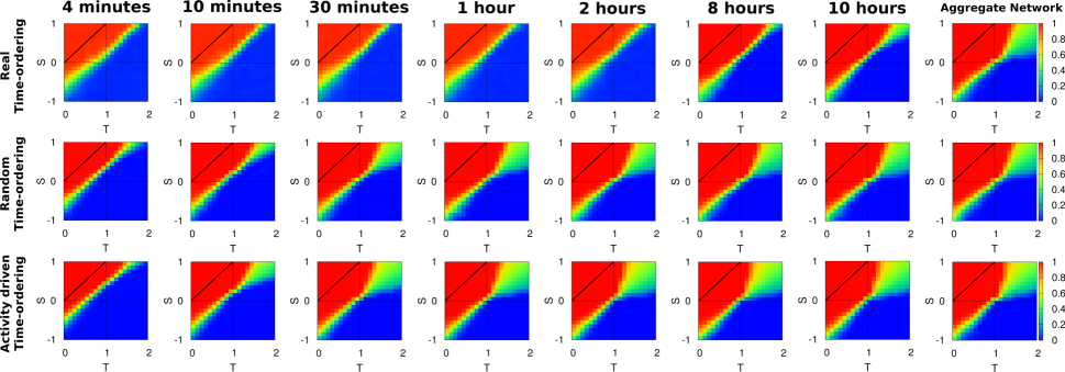
Figure 3: (Color online). Cooperation diagrams for the INFOCOM data set. Fraction of cooperators at the equilibrium as a function of the temptation to defect (T) and of the sucker’s score (S) for different values of the interval $\Delta t$ between two successive strategy updates. From left to right, the diagrams correspond to $\Delta t$ equal to 4 minutes, 10 minutes, 30 minutes, 1 hour, 2 hours, 8 hours, 10 hours, and $M\tau\simeq 4$ days. The top, middle, and bottom row report, respectively, the results for the original data set, the reshuffled time-varying graph, and synthetic graphs constructed through the activity-driven model. The results are averaged over 50 different realizations. Red (light gray) corresponds to $100\%$ of cooperators, while blue (dark gray) indicates $100\%$ defectors. As in Fig. 2, the comparison of the diagrams corresponding to the same update interval shows that differences appear in the region that separates the full cooperation and full defection phases and that these differences favor (in terms of degree of cooperation) the randomized and synthetic sequences. See Fig. 9 for additional details.

III Evolution of Cooperation in Time-varying Networks

III.1 Cooperation Diagrams

To simulate the game on a time-varying topology $\{G_{m}\}_{m=1,\ldots,M}$, we start from a random distribution of strategies, so that each individual initially behaves either as a cooperator or as a defector, with equal probability. The simulation proceeds in rounds, where each round consists of a playing stage followed by a strategy update. In the first stage, each agent plays with all her neighbors on the first graph of the sequence, namely on $G_{1}$, and accumulates the payoff according to the matrix in Eq. (1). Then the graph changes, and the agents employ the same strategies to play with all their neighbors in the second graph of the sequence, $G_{2}$. The new payoffs are summed to those obtained in the previous iteration. The same procedure is then repeated $n$ times with $n$ such that $n\tau$ is equal to a chosen interval $\Delta t$, which is the strategy update interval. At this point, the playing stage terminates and agent strategies are updated following the Fermi update in Eq. (2). After the agents have updated their strategy, their payoff is reset to $0$ and they start another round, during the subsequent time interval of length $\Delta t=n\tau$, as described above.

To evaluate the degree of cooperation obtained for a given value of the strategy update interval $\Delta t$ and a pair of values $(T,S)$, we compute the average fraction of cooperators $\langle C(T,S)_{\Delta t}\rangle$:

$$\langle C(T,S)_{\Delta t}\rangle=\dfrac{1}{Q}\sum_{i=1}^{Q}\dfrac{N_{c}^{i}}{N}\,,$$ (3)

where $N_{c}^{i}$ is the number of cooperators found at time $i\,\Delta t$ and $Q$ is the total number of rounds played. In general, we set $Q$ large enough to guarantee that the system reaches a stationary state in which the level of cooperation remains roughly constant.

We have simulated the system using different values of $\Delta t$. Notice that for smaller value of $\Delta t$, the time scale of the strategy update is comparable with that of the graph evolution, while when $\Delta t$ is equal to the entire observation period $M\tau$ the game is effectively played on a static topology, namely the weighted aggregated graph corresponding to the whole observation interval. We focus now on the top panels of Figs. 2 and 3, where we show how the average fraction of cooperators depends on the parameters $S$ and $T$ and on the length $\Delta t$ of the strategy update interval. We considered six values of $\Delta t$ for the MIT data set, from $\Delta t=1$ hour up to the whole observation interval, and eight values for INFOCOM’06, ranging from minutes up to the aggregate network.

At first glance, we notice that the rightmost diagrams in both figures, which correspond to $\Delta t=M\tau$, are in perfect agreement with the results of evolutionary games played on static topologies reported in the literature (see, e.g., pachpnas ; anxorev ). If we look at the cooperation diagrams obtained by increasing the value of $\Delta t$ in the original sequences of graphs (top panels of Figs. 2 and 3), we notice an increase of the area of the red region, which corresponds to configurations in which 100% of the nodes are cooperators at the stationary state. In particular, for MIT Reality Mining (Fig. 2), the fraction of cooperators increases up until $\Delta t=2$ months, after which the cooperation diagram is practically indistinguishable from that obtained on the static aggregated graph.

As we pointed out above, edge activation patterns show non-trivial correlations. To highlight the effects of temporal correlations and of periodicity in the appearance of links in the real data sets, we have simulated the games also on randomized time-varying graphs and on synthetic networks generated through the activity-driven model Perra2012 (See Appendix B for details on the activity-driven model). The results for randomized graphs and activity-driven graphs are reported, respectively, in the middle and in bottom panels of Figs. 2 and 3.

Randomized time-varying graphs are obtained by uniformly reshuffling the original sequences of snapshots. In this case, the frequency of each pairwise contact is preserved equal to that of the original data set. However, the temporal correlations of these contacts, namely the persistence of an edge during consecutive time snapshots, are completely wiped out. As expected, for $\Delta t=M\tau$ the cooperation diagrams obtained on the reshuffled sequences (middle rightmost panels of Figs. 2 and 3) are identical to those obtained on the corresponding original data sets (top rightmost panels). In fact, when $\Delta t=M\tau$ each agent plays with all the contacts she has seen in the whole observation interval, with the corresponding weights, before updating her strategy, and thus the frequencies of contacts are the only ingredients responsible for the emergence of cooperation. Conversely, for smaller values of $\Delta t$, the importance of the temporal correlations of each pairwise contact becomes clear since the cooperation diagrams for randomized and original networks are very different in both data sets. In fact, for the randomized graphs, the cooperation levels at $\Delta t=1$ week and $\Delta t=2$ hours for the Reality and INFOCOM data sets, respectively, are comparable to those for $\Delta t=M\tau$. This points out that cooperation is enhanced by destroying the temporal correlations of pairwise contacts.

Little differences are observed between activity-driven synthetic networks and the corresponding graph sequence randomizations (results shown in the bottom panels of Figs. 2 and 3). In this case not only are temporal correlations wiped out, but also the microscopic structure of each snapshot is replaced by a graph having a similar density of links. This rewiring distributes links more heterogeneously than in the original and the randomized sequences (see Appendix B for details). The cooperation diagrams of activity-driven networks show a further increase of the cooperation levels for even smaller values of the strategy update interval, $\Delta t$, than in the case of Random graphs. Namely, for $\Delta t=1$ day in Reality Mining (Fig. 2) and for $\Delta t=30$ minutes in INFOCOM (Fig. 3), we already recover the cooperation levels of $\Delta t=M\tau$. These results indicate that defectors take advantage of the volatility of edges, and that cooperation emerges only when the interval between two consecutive strategy updates is large enough. A more detailed visualization of the differences between the phase diagrams obtained in the original sequence for different values of $\Delta t$ and those observed for the randomized and synthetic networks is reported in Figs. 8 and 9.

III.2 Structural analysis of time varying networks

The reported results suggest that the ordering, persistence, and distribution of edges over consecutive time windows are all fundamental ingredients for the success of cooperation. In general, a small value of $\Delta t$ in the original data sets corresponds to playing the game on a sparse graph, possibly comprising a number of small components, in which nodes are connected to a small neighborhood that persists rather unaltered over consecutive time windows. The small size of the isolated clusters and the persistence of the connections within them allow defectors to spread their strategy efficiently. In the following, we will test this hypothesis by characterizing the structure of the original and randomized versions of the time-varying graphs.

In order to investigate the dependence of cooperation on the strategy update interval $\Delta t$, we computed the average fraction $\langle\mathcal{S}\rangle$ of nodes in the giant component of the graphs as a function of $\Delta t$ for the original data sets and for the reshuffled and synthetic sequences of snapshots. The results reported in Fig. 4 indicate that for a given value of $\Delta t$, the giant component of graphs in the randomized sequences or in the activity-driven model is larger than that of graphs in the original ordering. The lack of temporal correlations between consecutive time snapshots in randomized and activity-driven networks produces an increase in the number of ties between different agents of the population even for small values of $\Delta t$. In addition, the more homogeneous distribution of links within the snapshots of the activity-driven network further increases the mixing of the agents and thus enlarges the size of the giant connected component compared to that of randomized graphs.

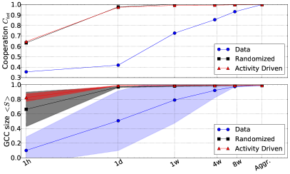
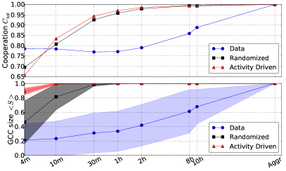
Figure 4: (Color online). Cooperation level and size of the Giant Component. Overall cooperation level $C_{tot}(\Delta t)$ and average size of the giant component $\langle\mathcal{S}\rangle$ as a function of the aggregation interval $\Delta t$ for MIT Reality Mining (top panels) and INFOCOM’06 (bottom panels). Blue circles correspond to the original data, black squares to the reshuffled networks and red triangles to the activity-driven model. The shades indicate the standard deviation of $\langle\mathcal{S}\rangle$ across the sequence of graphs for each value of $\Delta t$. Notice that the typical size of the giant component at time-scale $\Delta t$ correlates quite well with the observed cooperation level at the same time-scale.

In Fig. 4, we also show the overall level of cooperation observed at a given aggregation scale $\Delta t$, $C_{\text{tot}}(\Delta t)$, defined as:

$$C_{\text{tot}}(\Delta t)=\frac{1}{C_{\text{tot}}(M\tau)}\int_{0}^{2}\!\!\!\mathrm{d}T\!\int_{-1}^{1}\!\!\!C(T,S)\,\mathrm{d}S\,.$$

Notice that $C_{\text{tot}}(\Delta t)$ is divided by the value $C_{\text{tot}}(M\tau)$ corresponding to the whole observation interval, so that $C_{\text{tot}}\in[0,1]$. The value of $\Delta t$ at which $\langle\mathcal{S}\rangle$ is comparable with the number of nodes $N$, i.e. when $\langle\mathcal{S}\rangle\simeq 1$, coincides with the value of $\Delta t$ at which the cooperation diagram becomes indistinguishable from that obtained for the aggregate network, $C_{\text{tot}}(\Delta t)\simeq 1$, for both the original and the reshuffled sequences of snapshots. This result confirms that the size of the giant connected component of the graph corresponding to a given aggregation interval plays a central role in determining the level of cooperation sustainable by the system, in agreement with the experiments discussed in wang_scirep_2012 for the case of static complex networks.

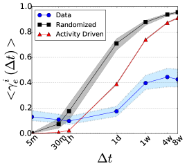
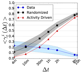
Figure 5: (Color online). Extremal temporal clustering $\gamma_{e}^{i}$ as a function of the strategy update interval $\Delta t$ on real data sets (blue dots). Top (bottom) panel refers to Reality Mining (INFOCOM). Black squares correspond to randomly reshuffled sequences and red triangles to activity-driven synthetic networks. In both data sets we notice that, for small values of $\Delta t$, real data display an higher value of clustering (persistence) than synthetic cases followed by a transition value of $\Delta t$ above which we observe a rapid increase in the clustering of synthetic cases such that the previous situation is inverted.

We also investigate the role of edge correlations between consecutive graphs on the observed cooperation level. To this aim, we analyze the temporal clustering $\gamma_{e}^{i}$ (see Appendix C), which captures the average tendency of edges to persist over time. In Fig. 5 we plot the evolution of the temporal clustering as a function of the strategy update interval $\Delta t$. The results clearly reveal that, for small values $\Delta t$, the persistence of ties in the two original data sets is larger than in the randomized and the activity-driven graphs. Overall, for small $\Delta t$, the large temporal clustering and the small average size of the giant component indicate that the graphs are composed of small clusters of nodes whose composition changes very slowly compared to the faster mixing observed in the randomized sequences. Thus, these are two ingredients hindering the cooperation levels in the original data sets: the size of the giant component, and the internal arrangement of connections within the different components.

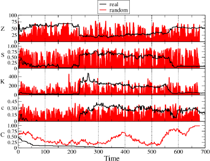
Figure 6: (Color online). Evolution of cooperation and topological quantities as a function of time $t$ for the INFOCOM data set in the Harmony Game ($T=0.9,S=0.2$). From top to bottom we display the number of components $Z$, fraction of nodes in the giant component $S$, number of links $K$, topological clustering coefficient $c$, and fraction of cooperators $C$ as a function of time. Black (red or gray in b/w) line corresponds to the original (randomized) data set.

As an example of the negative effect on cooperation of the combination of the two latter ingredients, we consider a pair of $\left(T,S\right)$ values in the Harmony Game (HG) regime ($0<T<1$ and $0<S<1$). The evolutionary dynamics of the HG in the well mixed (all-to-all) regime drives the system towards full cooperation. Even though this regime is the best scenario for the promotion of cooperation, the real time varying graphs exhibit small cooperation levels for small $\Delta t$. This is mainly due to the high level of segregation of interactions in disconnected and small clusters. Under these conditions (far from the well mixed hypothesis), the HG behaves differently in the regimes $T<S$ and $S<T$ (these two regimes are separated by the solid line $S=T$ in the panels of Figs. 2 and 3). While in the first regime, $T<S$, the pairwise encounters between a cooperator and a defector yield more benefit to the former, this is not the case when $S<T$. Thus, when the population is segregated into small (and persistent) clusters containing a small number of nodes, defection easily prevails in the region $S<T$ of the HG. This counterintuitive result is obtained for the original time varying graphs (especially for that of MIT) and small $\Delta t$. The time evolution of the interaction patterns of the real data sets confirms the structural roots of this behavior.

In Fig. 6 we display, for the case of INFOCOM, the number of components $Z$, the number of links $K$, the size of the giant component $S$, and the topological clustering coefficient $c$ (i.e. the probability that two neighbors of a given node are also connected) as a function of time $t$. Similar results are obtained for the MIT data set. We notice considerable differences between the time evolution of these quantities in the original time series and in the randomized ones. Namely, in the original time-varying graph we observe a long initial time window during which the real network displays a large number of components and poor connectivity. This period is then followed by another long period characterized by the appearance of a connected and clustered giant component. As expected, the randomized graph does not show this persistent behavior. In the bottom panel, we show the evolution of cooperation when the update interval is set to its minimum value, $\Delta t=4$ minutes. As can be observed, starting at time $0$ would imply that the initial fraction of cooperators face a rather complicated scenario for their survival even in the HG regime.

Turning our attention back to Fig. 5, we notice that, as $\Delta t$ increases, the link persistence grows similarly in the randomized and activity-driven networks. This growth points out that the randomization of snapshots in one null model and the redistribution of links in the other one make the ties more stable as $\Delta t$ increases. This stabilization, however, does not lead to a decrease in cooperation since it is combined with the fast increase with $\Delta t$ of the size of the giant component.

IV Conclusions

Although the impact of network topology on the onset and persistence of cooperation has been extensively studied in recent years, the recent availability of data sets with time-resolved information about social interactions allows for a deeper investigation of the impact of time-evolving social structures on evolutionary dynamics. Here we addressed two crucial questions: does the interplay between the time scale associated with graph evolution and that corresponding to the strategy update affect the classical results about the enhancement of cooperation driven by network reciprocity? And what is the role of the time correlations of temporal networks in the evolution of cooperation? The importance of the competition between the time scale of social ties and their corresponding outcome (here the games played and the benefits obtained) and the update of strategies have been recently addressed cuesta ; pachtraul . However, in our work we attempted to go one step further by relying on two empirical data sets incorporating the two ingredients whose impact over the evolution of cooperation we want to evaluate: the time scale of social interactions and their temporal correlations.

Our results confirm that, for all four social dilemmas studied in this work, cooperation is seriously hindered when (i) agent strategy is updated too frequently with respect to the typical time scale of agent interaction, and (ii) realistic link temporal correlations are present. This phenomenon is a consequence of the relatively small size of the giant component of the graphs obtained at small aggregation intervals. However, when the temporal sequence of social contacts is replaced by randomized or synthetic time-varying networks preserving the original activity attributes of links or nodes but breaking the original temporal correlations, the structural patterns of the network at a given time scale of strategy update changes dramatically from those observed in real data. As a consequence, the effects of temporal resolution over cooperation are smoothed and, by breaking the real temporal correlations of social contacts, cooperation can emerge and persist even for moderately small time periods between consecutive strategy updates.

Our findings suggest that the frequency at which the connectivity of a given system is sampled has to be carefully chosen, according with the typical time scale of the social interaction dynamics. For instance, as stock brokers might decide to change strategy after just a couple of interactions, other processes such as trust formation in business or collaboration networks are likely to be better described as the result of multiple subsequent interactions. These conclusions are also supported by the results of a recent paper by Ribeiro et al. ribeiro2013 in which the effects of temporal aggregation interval $\Delta t$ in the behavior of random walks are studied. One limitation of the current work comes from the fact that the used data sets have not been specifically collected in order to study cooperation spreading on networks and might represent therefore a suboptimal network substrate for the dynamical process under study. At the same time, these empirical data sets arguably contain the most direct measurement of human interaction upon which any social interaction mechanism is then built up and –already at this simple level of face-to-face interaction– contain rich and non-trivial structures and phenomena. One example of this is the fundamental role played by the real-data time correlations in dynamical processes on the graph, which calls for more models of temporal networks and for a better understanding of their nature. In a nutshell, our results point out that one should always bear in mind that both the over- and the under-sampling of time-evolving social graph and the use of the finest/coarsest temporal resolution could substantially bias the results of a game-theoretic model defined on the corresponding network. These results pave the way to a more detailed investigation of social dilemmas in systems where both structural and temporal correlations are incorporated in the interaction maps.

Appendix A Data sets Description

In the following, we introduce the principal characteristics of the two data sets used in our study. As stated in the main text, one of the reasons behind the emergence of cooperation is the persistence of interactions. A way to gauge such persistence is measuring the autocorrelation function $R$ of our time series as shown in Fig. 7.

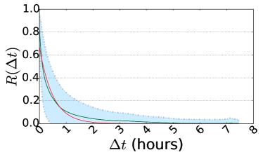
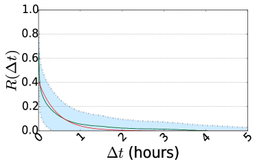
Figure 7: (Color online). Autocorrelation fucntion $R$ for edge activations, averaged over all the active edges in the data sets, Reality (top) and INFOCOM (bottom). The long lasting correlations in the edge activity of both data sets (up to 6-8 hours for Reality and 3-4 hours for INFOCOM) represent one of the main ingredients behind the different cooperation outcomes. Red (gray) line corresponds to the exponential fit of the data.

A.1 MIT Reality Mining data set

The data set describes proximity interactions collected through the use of Bluetooth-enabled phones eaglepentland . The phones were distributed to a group of 100 users, composed by 75 MIT Media Laboratory students and 25 faculty members. Each device had a unique tag and was able to detect the presence and identity of other devices within a range of 5–10 meters. The interactions, intended as proximity of devices, were recorded over a period of about six months. In addition to the interaction data, the original data set included also information regarding call logs, other Bluetooth devices within detection range, the cell tower to which the phones were connected, and information about phone usage and status. Here, we consider only the contact network data, ignoring any other contextual metadata. The resulting time-varying network is an ordered sequence of 41291 graphs, each having N=100 nodes. Each graph corresponds to a proximity scan taken every 5 minutes. An edge between two nodes indicates that the two corresponding devices were within detection range of each other during that interval. We refer to such links as active. During the entire recorded period, 2114 different edges have been detected as active, at least once. This corresponds to the aggregate graph having a large average node degree $\langle k\rangle\simeq 42$. However, this is an artefact of the aggregation; the single snapshots tend to be very sparse, usually containing between 100 and 200 active edges.

A.2 INFOCOM’06 data set

The data set consists of proximity measurements collected during the IEEE INFOCOM’06 conference held in a hotel in Barcelona in 2006 scott . A sample of $78$ participants from a range of different companies and institutions were chosen and equipped with a portable Bluetooth device, Intel iMote, able to detect similar devices nearby. Area “inquiries” were performed by the devices every 2 minutes, with a random delay or anticipation of 20 seconds. The delay/anticipation mechanism was implemented in order to avoid synchronous measurements, because, while actively sweeping the area, devices could not be detected by other devices. A total number of 2730 distinct edges were recorded as active at least once in the observation interval, while the number of edges active at a given time is significantly lower, varying between 0 and 200, depending on the time of the day.

Appendix B Activity-driven model

The activity-driven model, introduced in Ref. Perra2012 , is a simple model to generate time-varying graphs starting from the empirical observation of the activity of each node, in terms of number of contacts established per unit time. Given a characteristic time-window $\Delta t$, one measures the activity potential $x_{i}$ of each agent $i$, defined as the total number of interactions (edges) established by $i$ in a time-window of length $\Delta t$ divided by the total number of interactions established on average by all agents in the same time interval. Then, each agent is assigned an activity $a_{i}=\eta x_{i}$, which is the probability per unit time to create a new connection or contact with any another agent $j$. The coefficient $\eta$ is a rescaling factor, whose value is appropriately set in order to ensure that the total number of active nodes per unit time in the system is equal to $\eta\langle x\rangle N$, where $N$ is the total number of agents. Notice that $\eta$ effectively determines the average number of connections in a temporal snapshot whose length corresponds to the resolution of the original data set.

The model works as follows. At each time $t$ the graph $G_{t}$ starts with $N$ disconnected nodes. Then, each node $i$ becomes active with probability $a_{i}\Delta t$ and connects to $m$ other randomly selected nodes. At the following time-step, all the connections in $G_{t}$ are deleted, and a new snapshot is sampled.

Notice that time-varying graphs constructed through the activity-driven model preserve the average degree of nodes in each snapshot, but impose that connections have, on average, a duration equal to $\Delta t$, effectively removing any temporal correlation among edges.

For the networks studied, we obtain mean raw activities $\langle x\rangle_{Infocom}\simeq 0.49$ and $\langle x\rangle_{Reality}\simeq 0.15$. Choosing a number $m=2$ of new links created for every activated node and constraining the average fraction of active nodes and the average number of contacts per node to be those of the real networks, we obtain $\eta_{Reality}\simeq 0.024$ and $\eta_{Infocom}\simeq 0.7$. Finally, the average activity of nodes becomes $\langle a\rangle_{Reality}=0.004\pm 0.001$ and $\langle a\rangle_{Infocom}=0.35\pm 0.11$.

The aggregated versions of networks obtained from the activity-driven model were computed in two steps: $i)$ a synthetic temporal network was created at the same temporal resolution and of the same length as the original data set; $ii)$ the synthetic network was aggregated on the appropriate time-window. This was done in order to mimic as closely as possible the procedure that we performed on the real networks, where a single temporal network was compared with its own aggregated versions.

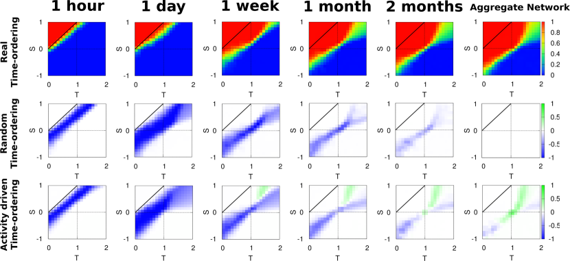
Figure 8: (Color online). Here we report with a color-code the difference between the cooperation diagram corresponding to the original MIT Reality Mining graph sequence (top panels) and those obtained on the reshuffled (middle panels) and synthetic networks (bottom panels), at different values of the update interval $\Delta t$.

Appendix C Temporal clustering

Several metrics have been lately proposed to measure the tendency of the edges of a time-varying graph to persist over time. One of the most widely used is the unweighted temporal clustering, introduced in Ref. tang_sw , which for a node $i$ of a time-varying graph is defined as:

$${\gamma}^{i}=\frac{1}{T-1}\sum_{t=1}^{T-1}\frac{\sum_{j}{a}^{t}_{ij}{a}_{ij}^{t+1}}{\sqrt{k_{i}^{t}k_{i}^{t+1}}}\,,$$ (4)

where $a_{ij}^{t}$ are the elements of the adjacency matrix of the time-varying graph at snapshot $t$, $k_{i}^{t}$ is the total number of edges incident on node $i$ at snapshot $t$, and $T$ is the duration of the whole observation interval. Notice that $\gamma^{i}$ takes values in $[0,1]$. In general, a higher value of $\gamma^{i}$ is obtained when the interactions of node $i$ persist longer in time, while $\gamma^{i}$ tends to zero if the interactions of $i$ are highly volatile.

If each snapshot of the time-varying graph is a weighted network, where the weight $\omega^{t}_{ij}$ represents the strength if the interaction between node $i$ and node $j$ at time $t$, we can define a weighted version of the temporal clustering coefficient as follows:

$${\gamma}_{w}^{i}=\frac{1}{T-1}\sum_{t=1}^{T-1}\frac{\sum_{j}{\omega}^{t}_{ij}{\omega}_{ij}^{t+1}}{s_{i}^{t}s_{i}^{t+1}}\,.$$ (5)

Finally, if we focus more on the persistence of interaction strength across subsequent network snapshots, we can define the extremal temporal clustering as:

$${\gamma}_{e}^{i}=\frac{1}{T-1}\sum_{t=1}^{T-1}\frac{\sum_{j}\min({\omega}^{t}_{ij},{\omega}_{ij}^{t+1})}{\sqrt{s_{i}^{t}s_{i}^{t+1}}}\,,$$ (6)

where by considering the minimum between ${\omega}^{t}_{ij}$ and ${\omega}_{ij}^{t+1}$ one can distinguish between persistent interactions having constant strength over time and those interactions having more volatile strength. As in our case social interactions are seen to be highly volatile in real data sets, the extremal version of the temporal clustering seems to be the best choice to unveil the persistence of social ties at short time scales.

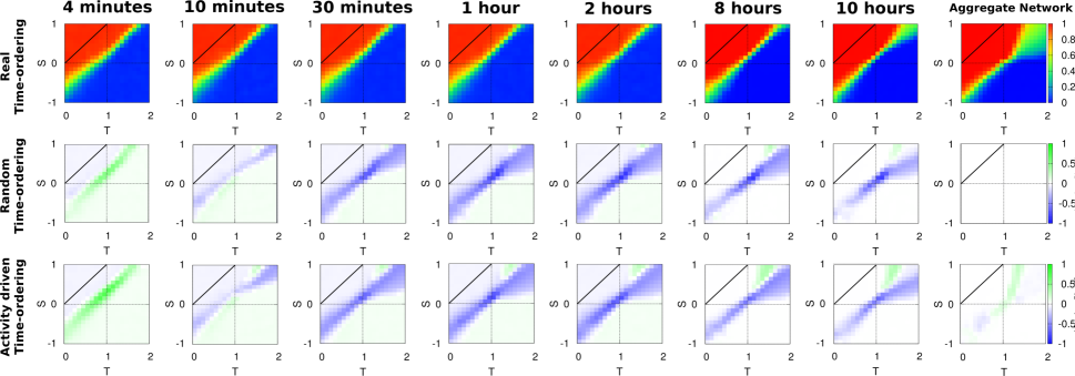
Figure 9: (Color online). As in Fig.8, we report the differences between the cooperation diagram corresponding to the original INFOCOM’06 data set and those obtained on the reshuffled (middle panels) and synthetic networks (bottom panels), at different values of the update interval $\Delta t$.

Appendix D Differences in the Cooperation Diagrams

To highlight the effects that temporal correlations between pairwise interactions have on the emergence of cooperation, we show in this appendix the quantitative differences among the cooperation level of the original data sets (as displayed by the fraction of cooperators as a function of $T$ and $S$) and both their randomized and activity-driven versions. In Figs. 8 and 9 we show these differences for the MIT Reality Mining and INFOCOM’06 graphs, respectively.

From these two figures, it becomes clear that most of the differences with the dynamics run on the original time-varying graph are concentrated at the interface between the regions in which 100% of the nodes are cooperators [the red (light gray) areas in the top panels] and those where 100% of the nodes become defectors [blue (dark gray) areas in the top panels]. Interestingly, for both data sets these differences are more pronounced for smaller values of $\Delta t$ and become less evident when $\Delta t$ increases, until they almost disappear for the largest aggregation interval.

References

- (1) E. Pennisi, “How did cooperative behavior evolve?”, Science 309, 93 (2005).
- (2) E. Pennisi, “On the origin of cooperation”, Science 325, 1196–1199 (2009).
- (3) J. Maynard-Smith and E. Szathmary, “The Major Transitions in Evolution” (Freeman, Oxford, UK, 1995).
- (4) M.A. Nowak, “Evolutionary Dynamics: Exploring the Equations of Life.” (The Belknap Press of Harvard University Press, Cambridge, MA, 2006).
- (5) P. Kollock, “Social dilemmas: the anatomy of cooperation”, Annu. Rev. Sociol. 24, 183–214 (1998).
- (6) J. Maynard-Smith, and G.R. Price, “The logic of animal conflict”, Nature 246 (5427), 15–18 (1973).
- (7) J. Maynard-Smith, “Evolution and the Theory of Games”, Cambridge Univ. Press, Cambridge (UK), (1982).
- (8) H. Gintis, “Game Theory Evolving” (Princeton University Press, Princeton, NJ, 2009).
- (9) L. Samuelson, “Evolution and game theory”, J. Econ. Perspect. 16, 47–66 (2002).
- (10) D.J. Watts, and S.H. Strogatz, “Collective dynamics of small-world networks” Nature 393, 440–442 (1998).
- (11) S.H. Strogatz, “Exploring complex networks” Nature 410, 268–276 (2001).
- (12) R. Albert, and A-L Barabási, “Statistical mechanics of complex networks”, Rev. Mod. Phys. 74, 47–97 (2002).
- (13) M.E.J. Newman, “The Structure and Function of Complex Networks” SIAM Rev. 45, 167–256 (2003).
- (14) S. Boccaletti, V. Latora, Y. Moreno, M. Chavez, and D-U Hwang, “Complex Networks: Structure and Dynamics”, Phys. Rep. 424, 175–308 (2006).
- (15) S.N. Dorogovtsev, A.V. Goltsev, and J.F.F. Mendes, “Critical phenomena in complex networks”, Rev Mod. Phys. 80, 1275–1335 (2008).
- (16) C. Castellano, S. Fortunato, and V. Loreto, “Statistical physics of social dynamics”, Rev. Mod. Phys. 81 591–646 (2009).
- (17) F.C. Santos, and J.M. Pacheco, “Scale-Free Networks Provide a Unifying Framework for the Emergence of Cooperation”, Phys. Rev. Lett. 95, 098104 (2005).
- (18) F.C. Santos, J.M. Pacheco, and T. Lenaerts, “Evolutionary dynamics of social dilemmas in structured heterogeneous populations”, Proc. Natl. Acad. Sci. (U.S.A.) 103, 3490–3494 (2006).
- (19) J. Gómez-Gardeñes, M. Campillo, L.M. Floría, and Y. Moreno, “Dynamical Organization of Cooperation in Complex Topologies”, Phys. Rev. Lett. 98, 108103 (2007).
- (20) S. Assenza, J. Gómez-Gardeñes, and V. Latora, “Enhancement of cooperation in highly clustered scale-free networks”, Phys. Rev. E 78, 017101 (2008).
- (21) F.C. Santos, M.D. Santos, and J.M. Pacheco, “Social diversity promotes the emergence of cooperation in public goods games”, Nature 454, 213–216 (2008).
- (22) J. Gómez-Gardeñes, M. Romance, R. Criado, D. Vilone, and A. Sánchez, “Evolutionary games defined at the network mesoscale: The Public Goods game”, Chaos 21, 016113 (2011).
- (23) M. Perc, J. Gómez-Gardeñes, A. Szolnoki, L. M. Floria, and Y. Moreno, “Evolutionary dynamics of group interactions on structured populations: a review”, J. Roy. Soc. Interface 10, 20120997 (2013).
- (24) G. Szabó, and G. Fáth, “Evolutionary games on graphs”, Phys. Rep. 446, 97 (2007).
- (25) M.D. Jackson, “Social and Economic Networks” (Princeton Univ. Press, Princeton, NJ, 2008).
- (26) C.P. Roca, J. Cuesta, and A. Sánchez, “Evolutionary game theory: temporal and spatial effects beyond replicator dynamics”, Phys. Life Rev. 6, 208 (2009).
- (27) M. Perc, and A. Szolnoki, “Coevolutionary games - A mini review”, BioSystems 99, 109–125 (2010).
- (28) T. Gross, and B. Blasius, “Adaptive coevolutionary networks: a review”, J. R. Soc. Interface 5, 259–271 (2008).
- (29) N. Eagle and A. Pentland, “Reality mining: sensing complex social systems”, Person. Ubiq. Comput. 10, 255–268 (2006).
- (30) J. Scott et al. , “CRAWDAD Trace”, INFOCOM, Barcelona (2006).
- (31) L. Isella, M. Romano, A. Barrat, C. Cattuto, V. Colizza, et al. , “Close Encounters in a Pediatric Ward: Measuring Face-to-Face Proximity and Mixing Patterns with Wearable Sensors.” PLoS ONE 6, e17144 (2011).
- (32) J. Stehle, N. Voirin, A. Barrat, C. Cattuto, L. Isella, et al. “High-Resolution Measurements of Face-to-Face Contact Patterns in a Primary School.” PLoS ONE 6, e23176 (2011).
- (33) L. Isella, J. Stehlé, A. Barrat, C. Cattuto, J-F Pinton, and W. Van den Broeck, “What’s in a crowd? Analysis of face-to-face behavioral networks”, J. Theor. Biol. 271, 166–180 (2011).
- (34) M. Karsai, M Kivelä, R.K. Pan, K. Kaski, J. Kertész, A-L Barabási, and J. Saramäki, “Small But Slow World: How Network Topology and Burstiness Slow Down Spreading”, Phys. Rev. E 83, 025102(R) (2011).
- (35) A-L Barabási, “The origin of bursts and heavy tails in human dynamics” Nature 435, 207–211 (2005).
- (36) J. Stehlé, A. Barrat, and G. Bianconi, “Dynamical and bursty interactions in social networks”, Phys. Rev. E 81, 035101(R) (2010).
- (37) M.C. González, C.A. Hidalgo, and A-L Barabási, “Understanding individual human mobility patterns” Nature 453, 779–782 (2008).
- (38) M. Szell, R. Lambiotte, and S. Thurner, “Multi-relational Organization of Large-scale Social Networks in an Online World”, Proc. Natl. Acad. Sci. (U.S.A.) 107, 13636–13641 (2010).
- (39) M. Szell, R. Sinatra, G. Petri, S. Thurner, and V. Latora, “Understanding mobility in a social petri dish”, Sci. Rep. 2, 457 (2012).
- (40) G. Kossinets, J. Kleinberg, and D. Watts, “The Structure of Information Pathways in a Social Communication Network,” Proceedings of the 14th ACM SIGKDD International Conference on Knowledge Discovery and Data Mining (ACM, New York, 2008).
- (41) V. Kostakos, “Temporal graphs”, Physica A 388, 1007–1023 (2009).
- (42) J. Tang, M. Musolesi, C. Mascolo, and V. Latora, “Temporal Distance Metrics for Social Network Analysis”, Proceedings of the 2nd ACM SIGCOMM Workshop on Online Social Networks (WOSN’09) (ACM, New York, 2009).
- (43) P. Holme and J. Saramäki, “Temporal networks”, Phys. Rep. 519, 97–125 (2012).
- (44) J. Tang, S. Scellato, M. Musolesi, C. Mascolo, and V. Latora, “Small-world behavior in time-varying graphs.” Phys. Rev. E 81, 055101(R) (2010).
- (45) V. Nicosia, J. Tang, C. Mascolo, M. Musolesi, G. Russo, V. Latora ”Graph Metrics for Temporal Networks”, edited by P. Holme and J. Saramäki, Temporal Networks. (Springer, Berlin, 2013), pp. 15-40.
- (46) R.K. Pan, and J. Saramäki, “Path lengths, correlations, and centrality in temporal networks,” Phys. Rev. E 84, 016105 (2011).
- (47) L. Kovanen, M. Karsai, K. Kaski, J. Kertesz, and J. Saramäki. “Temporal motifs in time-dependent networks” J. Stat. Mech., P11005 (2011).
- (48) J. Tang, M. Musolesi, C. Mascolo, V. Latora, and V. Nicosia, “Analysing Information Flows and Key Mediators through Temporal Centrality Metrics” Proceedings of the 3rd ACM Workshop on Social Network Systems (SNS’10), (ACM, New York, 2010).
- (49) V. Nicosia, J. Tang, M. Musolesi, G. Russo, C. Mascolo, and V. Latora, “Components in time-varying graphs”, Chaos 22, 023101 (2012).
- (50) P.J. Mucha, T. Richardson, K. Macon, M.A. Porter, and J-P Onnela, “Community structure in time-dependent, multiscale, and multiplex networks”, Science 328, 876–878 (2010).
- (51) M. Starnini, A. Baronchelli, A. Barrat, and R. Pastor-Satorras, “Random walks on temporal networks”, Phys. Rev. E 85, 056115 (2012).
- (52) N. Perra, A. Baronchelli, D. Mocanu, B. Gonçalves, R. Pastor-Satorras, and A. Vespignani, “Walking and searching in time-varying networks”, Phys. Rev. Lett. 109, 238701 (2012).
- (53) B. Ribeiro, N. Perra, and A. Baronchelli, “Quantifying the effect of temporal resolution on time-varying networks.” Sci. Rep. 3, 1 (2013).
- (54) L.E.C. Rocha, F. Liljeros, and P. Holme, “Simulated Epidemics in an Empirical Spatiotemporal Network of 50,185 Sexual Contacts.” PLoS Comp. Biol. 7, e1001109 (2011).
- (55) L.E.C. Rocha, A. Decuyper, and V.D. Blondel, “Epidemics on a stochastic model of temporal network”, Dynamics on and of Complex Networks, Volume 2. Modeling and Simulation in Science, Engineering and Technology (Springer, New York, 2013), pp. 301–314.
- (56) L.E.C. Rocha and V.D. Blondel, “Bursts of vertex activation and epidemics in evolving networks.” PLoS Comp. Biol. 9, e1002974 (2013).
- (57) N. Fujiwara, J. Kurths, and A. Díaz-Guilera, “Synchronization in networks of mobile oscillators.” Phys. Rev. E 83, 025101(R) (2011).
- (58) L.E. Blume, “The Statistical Mechanics of Strategic Interaction.” Games Econ. Behav. 5, 387 (1993).
- (59) G. Szabó and C. Töke, “Evolutionary prisoner’s dilemma game on a square lattice”, Phys. Rev. E 58, 69 (1998).
- (60) N. Perra, B. Gonçalves, R. Pastor-Satorras, and A. Vespignani, “Activity driven modeling of time varying networks”, Sci. Rep. 2, 469 (2012).
- (61) Z. Wang, A. Szolnoki, and M. Perc, “If players are sparse social dilemmas are too: Importance of percolation for evolution of cooperation.” Sci. Rep. 2, 369 (2012).
- (62) C.P. Roca, J.A. Cuesta, and A. Sánchez, “Time Scales in Evolutionary Dynamics”, Phys. Rev. Lett. 97, 158701 (2006).
- (63) J.M. Pacheco, A. Traulsen, and M.A. Nowak, “Coevolution of Strategy and Structure in Complex Networks with Dynamical Linking”, Phys. Rev. Lett. 97, 258103 (2006).