Inclusive tau lepton decay:
the effects due to hadronization

Abstract:

The inclusive $\tau$ lepton hadronic decay and its description within Dispersive approach to Quantum Chromodynamics are briefly discussed.

1 Introduction

The process of the inclusive $\tau$ lepton decay into hadrons constitutes a unique opportunity to explore the nonperturbative nature of the strong interaction at low energies. The experimental data on hadronic $\tau$ decay are commonly employed in various tests of Quantum Chromodynamics (QCD) and entire Standard Model, that puts strong limits on possible New Physics beyond the latter.

The pertinent experimentally measurable quantity is the ratio of the total width of $\tau$ lepton decay into hadrons to the width of its leptonic decay. Usually, this ratio is decomposed into several parts, specifically

$$R_{\tau}=\frac{\Gamma(\tau^{-}\to\mbox{hadrons}^{-}\,\nu_{\tau})}{\Gamma(\tau^{-}\to e^{-}\,\bar{\nu}_{e}\,\nu_{\tau})}=R_{\tau,\mbox{\tiny V}}^{\mbox{\tiny$J$=0}}+R_{\tau,\mbox{\tiny V}}^{\mbox{\tiny$J$=1}}+R_{\tau,\mbox{\tiny A}}^{\mbox{\tiny$J$=0}}+R_{\tau,\mbox{\tiny A}}^{\mbox{\tiny$J$=1}}+R_{\tau,\mbox{\tiny S}}.$$ (1)

In the right hand side of this equation the last term accounts for the $\tau$ lepton decay modes which involve strange quark, whereas the other terms account for the hadronic decay modes involving light quarks (u, d) only and associated with vector (V) and axial–vector (A) quark currents, respectively. The superscript $J$ indicates the angular momentum in the hadronic rest frame.

The quantities appearing in Eq. (1) can be evaluated by making use of the so–called spectral functions, which are extracted from the experiment. For the zero angular momentum ($J=0$) the vector spectral function vanishes (that leads to $R_{\tau,\mbox{\tiny V}}^{\mbox{\tiny$J$=0}}=0$), whereas the axial–vector one is commonly approximated by Dirac $\delta$–function, since the dominant contribution is due to the pion pole here. The experimental predictions [1, 2] for the nonstrange spectral functions corresponding to $J=1$ are presented in Fig. 1. In what follows we shall restrict ourselves to the consideration of terms $R_{\tau,\mbox{\tiny V}}^{\mbox{\tiny$J$=1}}$ and $R_{\tau,\mbox{\tiny A}}^{\mbox{\tiny$J$=1}}$ of $R_{\tau}$–ratio (1).

The aforementioned quantities can be represented in the following form

$$R_{\tau,\mbox{\tiny V/A}}^{\mbox{\tiny$J$=1}}=\frac{N_{\mbox{\scriptsize c}}}{2}\,|V_{\mbox{\scriptsize ud}}|^{2}\,S_{\!\mbox{\tiny EW}}\,\Bigl{(}\Delta^{\mbox{\tiny V/A}}_{\mbox{\tiny QCD}}+\delta^{\prime}_{\mbox{\tiny EW}}\Bigr{)},$$ (2)

where $N_{\mbox{\scriptsize c}}=3$ is the number of colors, $|V_{\mbox{\scriptsize ud}}|=0.97425\pm 0.00022$ is Cabibbo–Kobayashi–Maskawa matrix element [3], $S_{\!\mbox{\tiny EW}}=1.0194\pm 0.0050$ and $\delta^{\prime}_{\mbox{\tiny EW}}=0.0010$ stand for the electroweak corrections (see Refs. [4, 5]), and

$$\Delta^{\mbox{\tiny V/A}}_{\mbox{\tiny QCD}}=2\int_{m_{\mbox{\tiny V/A}}^{2}}^{M_{l}^{2}}\!\!\biggl{(}1-\frac{s}{M_{l}^{2}}\biggr{)}^{\!\!\!\!2}\!\biggl{(}1+2\frac{s}{M_{l}^{2}}\biggr{)}R^{\mbox{\tiny V/A}}(s)\,\frac{ds}{M_{l}^{2}}$$ (3)

denotes the QCD contribution to Eq. (2). In the integrand of Eq. (3)

$$R(s)=\frac{1}{2\pi i}\lim_{\varepsilon\to 0_{+}}\Bigl{[}\Pi(s+i\varepsilon)-\Pi(s-i\varepsilon)\Bigr{]},$$ (4)

where $\Pi(q^{2})$ is the hadronic vacuum polarization function

$$\Pi_{\mu\nu}(q^{2})=i\!\int\!d^{4}x\,\,e^{iqx}\langle 0|\,T\!\left\{J_{\mu}(x)\,J_{\nu}(0)\right\}|0\rangle=\frac{i}{12\pi^{2}}(q_{\mu}q_{\nu}-g_{\mu\nu}q^{2})\Pi(q^{2})$$ (5)

with $J_{\mu}(x)$ being the electromagnetic quark current (the indices “V” and “A” will only be shown when relevant hereinafter). It is worthwhile to mention that for practical purposes it is also convenient to deal with the so–called Adler function [6]

$$D(Q^{2})=-\frac{d\,\Pi(-Q^{2})}{d\ln Q^{2}},\qquad Q^{2}=-q^{2}=-s.$$ (6)

             

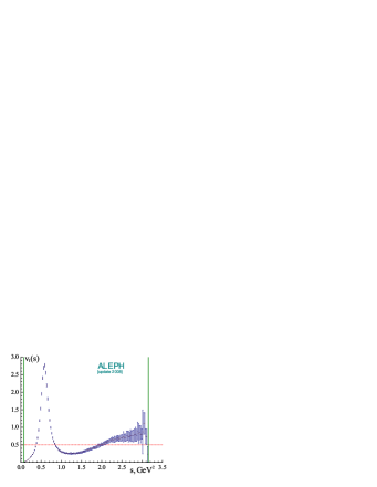
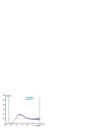
Figure 1: The inclusive $\tau$ lepton hadronic decay vector (left plot) and axial–vector (right plot) spectral functions [1, 2]. Vertical solid lines mark the boundaries of respective kinematic intervals, whereas horizontal dashed lines denote the naive massless parton model predictions.

It is necessary to outline that in Eq. (3) $M_{l}$ denotes the mass of the lepton on hand, whereas $m$ stands for the hadronic threshold mass (i.e., the total mass of the lightest allowed hadronic decay mode of this lepton in the corresponding channel). The nonvanishing value of $m$ explicitly expresses the physical fact that $\tau$ lepton is the only lepton which is heavy enough ($M_{\tau}\!\simeq\!\!1.777\,$GeV [3]) to decay into hadrons. Indeed, in the massless limit ($m=0$) the theoretical prediction for the QCD contribution (3) to Eq. (2) is nonvanishing for either lepton ($l=e,\mu,\tau$). Specifically, the leading–order term of Eq. (9) $\Delta^{\mbox{\scriptsize$(0)$}}_{\mbox{\scriptsize pert}}=1$ (which corresponds to the naive massless parton model prediction for the Adler function (8) $D^{\mbox{\scriptsize$(0)$}}_{\mbox{\scriptsize pert}}(Q^{2})=1$) does not depend on $M_{l}$, and, therefore, is the same for either lepton. In the realistic case (i.e., when the total mass of the lightest allowed hadronic decay mode exceeds the masses of electron and muon, $M_{e}<M_{\mu}<m<M_{\tau}$) Eq. (3) acquires non–zero value for the case of the $\tau$ lepton only.

2 Inclusive $\tau$ lepton hadronic decay within perturbative approach

In this Section we shall deal with the massless limit, that implies that the masses of all final state particles are neglected ($m=0$). By making use of definitions (4) and (6), integrating by parts, and additionally employing Cauchy theorem, the quantity $\Delta^{\mbox{\tiny}}_{\mbox{\tiny QCD}}$ (3) can be represented as

$$\Delta^{\mbox{\tiny}}_{\mbox{\tiny QCD}}=\frac{1}{2\pi}\!\int_{-\pi}^{\pi}\!D\bigl{(}M_{\tau}^{2}\,e^{i\theta}\bigr{)}\bigl{(}1+2e^{i\theta}-2e^{i3\theta}-e^{i4\theta}\bigr{)}d\theta,$$ (7)

see, e.g., Refs. [7, 4]. It is worth noting here that Eq. (7) is only valid for the massless limit of “genuine physical” Adler function $D^{\mbox{\scriptsize$$}}_{\mbox{\scriptsize phys}}(Q^{2})$, which possesses the correct analytic properties in the kinematic variable $Q^{2}$ (otherwise Eq. (7) can not be derived from Eq. (3)). However, in Eq. (7) one usually directly employs the perturbative approximation for the Adler function

$$D(Q^{2})\simeq D^{\mbox{\scriptsize$(\ell)$}}_{\mbox{\scriptsize pert}}(Q^{2})=1+\sum\nolimits_{j=1}^{\ell}d_{j}\Bigl{[}\alpha^{\mbox{\scriptsize$(\ell)$}}_{\mbox{\scriptsize pert}}(Q^{2})\Bigr{]}^{j},\qquad Q^{2}\to\infty,$$ (8)

which has unphysical singularities in $Q^{2}$. In this equation at the one–loop level (i.e., for $\ell=1$) the strong running coupling reads $\alpha^{\mbox{\scriptsize$(1)$}}_{\mbox{\scriptsize pert}}(Q^{2})=4\pi/[\beta_{0}\,\ln(Q^{2}/\Lambda^{2})]$, where $\beta_{0}=11-2n_{\mbox{\scriptsize f}}/3$, $\Lambda$ denotes the QCD scale parameter, $n_{\mbox{\scriptsize f}}$ is the number of active flavors, and $d_{1}=1/\pi$, see Ref. [8] for the details. In what follows the one–loop level with $n_{\mbox{\scriptsize f}}=3$ active flavors will be assumed. Eventually, Eq. (7) corresponding to the perturbative Adler function (8) takes the form

$$\Delta^{\mbox{\scriptsize$$}}_{\mbox{\scriptsize pert}}=\Delta^{\mbox{\scriptsize$(0)$}}_{\mbox{\scriptsize pert}}+\frac{4}{\beta_{0}}\!\int_{0}^{\pi}\frac{\lambda A_{1}(\theta)+\theta A_{2}(\theta)}{\pi(\lambda^{2}+\theta^{2})}\,d\theta,$$ (9)

where $\Delta^{\mbox{\scriptsize$(0)$}}_{\mbox{\scriptsize pert}}\!=\!1$, $A_{1}(\theta)\!=\!1\!+\!2\cos(\theta)\!-\!2\cos(3\theta)\!-\!\cos(4\theta)$, $A_{2}(\theta)\!=\!2\sin(\theta)\!-\!2\sin(3\theta)\!-\!\sin(4\theta)$, and $\lambda=\ln\bigl{(}M_{\tau}^{2}/\Lambda^{2}\bigr{)}$.

             

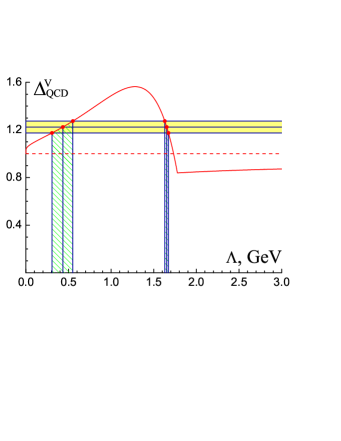
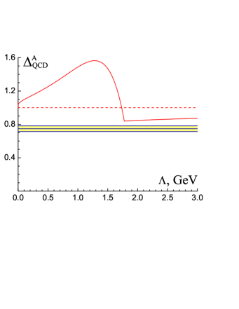
Figure 2: Juxtaposition of the one–loop perturbative expression $\Delta^{\mbox{\tiny$$}}_{\mbox{\tiny pert}}$ (9) (solid curve) with relevant experimental data (10) (horizontal shaded bands). The leading–order term $\Delta^{\mbox{\tiny$(0)$}}_{\mbox{\tiny pert}}=1$ (9) is denoted by dashed line. The solution for QCD scale parameter $\Lambda$ (if exists) is shown by vertical dashed band.

It is worthwhile to underscore that perturbative approach provides identical expressions (9) for the functions (3) in vector and axial–vector channels (i.e., $\Delta^{\mbox{\scriptsize$\mbox{\tiny V}$}}_{\mbox{\scriptsize pert}}\equiv\Delta^{\mbox{\scriptsize$\mbox{\tiny A}$}}_{\mbox{\scriptsize pert}}$). However, their experimental values [1, 2] are different, namely

$$\Delta^{\mbox{\scriptsize$\mbox{\tiny V}$}}_{\mbox{\scriptsize exp}}=1.224\pm 0.050,\qquad\Delta^{\mbox{\scriptsize$\mbox{\tiny A}$}}_{\mbox{\scriptsize exp}}=0.748\pm 0.034.$$ (10)

The comparison of these quantities with perturbative result (9) is presented in Fig. 2. As one can infer from this figure, for the vector channel there are two solutions for the QCD scale parameter: $\Lambda=\bigl{(}434^{+117}_{-127}\bigr{)}\,$MeV (which is usually retained) and $\Lambda=\bigl{(}1652^{+21}_{-23}\bigr{)}\,$MeV (which is commonly merely disregarded). As for the axial–vector channel, the perturbative approach fails to describe the experimental data [1, 2], since for any value of $\Lambda$ the function $\Delta^{\mbox{\scriptsize$$}}_{\mbox{\scriptsize pert}}$ (9) exceeds $\Delta^{\mbox{\scriptsize$\mbox{\tiny A}$}}_{\mbox{\scriptsize exp}}$ (10).

3 Dispersive approach to Quantum Chromodynamics

It is crucial to emphasize that the presented in Section 2 massless limit completely leaves out the effects due to hadronization, which play significant role in the studies of the strong interaction processes at low energies. Specifically, the mathematical realization of the physical fact, that in a strong interaction process no final state hadrons can be produced at energies below the hadronic threshold mass $m$, consists in the fact that the beginning of cut of corresponding hadronic vacuum polarization function $\Pi(q^{2})$ (5) in the complex $q^{2}$–plane is located at the threshold of hadronic production $q^{2}=m^{2}$, but not at $q^{2}=0$ (see also discussion of this issue in Ref. [9]). Such restrictions are inherently embodied within relevant dispersion relations, which, in turn, impose stringent physical intrinsically nonperturbative constraints on the quantities on hand.

The complete set of dispersion relations, which express the functions (4), (5), and (6) in terms of each other, reads

$$\Delta\Pi(q^{2},\,q_{0}^{2}) = (q^{2}-q_{0}^{2})\int_{m^{2}}^{\infty}\frac{R(\sigma)}{(\sigma-q^{2})(\sigma-q_{0}^{2})}\,d\sigma=-\int_{-q_{0}^{2}}^{-q^{2}}D(\zeta)\frac{d\zeta}{\zeta},$$ (11)

$$D(Q^{2}) = -\frac{d\,\Pi(-Q^{2})}{d\,\ln Q^{2}}=Q^{2}\int_{m^{2}}^{\infty}\frac{R(\sigma)}{(\sigma+Q^{2})^{2}}\,d\sigma,$$ (12)

$$R(s) = \frac{1}{2\pi i}\lim_{\varepsilon\to 0_{+}}\Bigl{[}\Pi(s+i\varepsilon)-\Pi(s-i\varepsilon)\Bigr{]}=\frac{1}{2\pi i}\lim_{\varepsilon\to 0_{+}}\int_{s+i\varepsilon}^{s-i\varepsilon}D(-\zeta)\frac{d\zeta}{\zeta},\qquad\quad$$ (13)

where $\Delta\Pi(q^{2},\,q_{0}^{2})=\Pi(q^{2})-\Pi(q_{0}^{2})$ and $s=q^{2}=-Q^{2}$ (see Refs. [6, 10]). For practical purposes, it proves to be convenient to deal with the integral representations, which express the aforementioned functions in terms of the common spectral density $\rho(\sigma)$. Such representations have been derived in the framework of Dispersive approach to QCD (see Refs. [11, 12] for the details):

$$\Delta\Pi^{(\ell)}(q^{2},\,q_{0}^{2}) = \Delta\Pi^{(0)}(q^{2},\,q_{0}^{2})+\!\int_{m^{2}}^{\infty}\rho^{(\ell)}(\sigma)\ln\biggl{(}\frac{\sigma-q^{2}}{\sigma-q_{0}^{2}}\frac{m^{2}-q_{0}^{2}}{m^{2}-q^{2}}\biggr{)}\frac{d\,\sigma}{\sigma},$$ (14)

$$D^{(\ell)}(Q^{2}) = D^{(0)}(Q^{2})+\frac{Q^{2}}{Q^{2}+m^{2}}\int_{m^{2}}^{\infty}\rho^{(\ell)}(\sigma)\frac{\sigma-m^{2}}{\sigma+Q^{2}}\frac{d\,\sigma}{\sigma},$$ (15)

$$R^{(\ell)}(s) = R^{(0)}(s)+\theta(s-m^{2})\int_{s}^{\infty}\rho^{(\ell)}(\sigma)\frac{d\,\sigma}{\sigma}.$$ (16)

In these equations $\theta(x)$ denotes the unit step–function ($\theta(x)=1$ if $x\geq 0$ and $\theta(x)=0$ otherwise) and $\rho^{(\ell)}(\sigma)$ is the $\ell$–loop spectral density:

$$\rho^{(\ell)}(\sigma)=\frac{1}{\pi}\frac{d}{d\,\ln\sigma}\,\mbox{Im}\lim_{\varepsilon\to 0_{+}}p^{(\ell)}(\sigma-i\varepsilon)=\frac{1}{\pi}\,\mbox{Im}\lim_{\varepsilon\to 0_{+}}d^{(\ell)}(-\sigma-i\varepsilon)=-\frac{d}{d\,\ln\sigma}\,r^{(\ell)}(\sigma),$$ (17)

with $p^{(\ell)}(q^{2})$, $d^{(\ell)}(Q^{2})$, and $r^{(\ell)}(s)$ being the $\ell$–loop strong corrections to functions (5), (6), and (4), respectively (see Refs. [11, 12] for the details).

It is worthwhile to note that integral representations (14)–(16) automatically embody all the nonperturbative constraints (including the correct analytic properties in the kinematic variable) that Eqs. (11)–(13) impose on the functions on hand. For example, dispersion relation (12) implies that the Adler function vanishes in the infrared limit ($D(Q^{2})\to 0$ at $Q^{2}\to 0$) and possesses the only cut along the negative semiaxis of real $Q^{2}$ starting at the hadronic production threshold $Q^{2}\leq-m^{2}$ (preliminary formulation of the Dispersive approach to QCD, which accounts for the second constraint only, was discussed in Ref. [13]).

It is worth mentioning also that integral representations (14)–(16) were obtained by making use of only the dispersion relations (11)–(13) and the fact that the strong correction $d(Q^{2})$ vanishes in the ultraviolet asymptotic $Q^{2}\to\infty$. Neither additional approximations nor model–dependent assumptions were involved in the derivation of Eqs. (14)–(16), see Refs. [11, 12] for the details. It is worthwhile to note that the hadronic vacuum polarization function (14) agrees with relevant lattice simulation data (e.g., Ref. [14]) and the Adler function (15) agrees with corresponding experimental prediction, see Refs. [11, 12] (as well as Ref. [15]) for the details.

In general, there is no unique way to calculate the spectral density (17) (see Refs. [16, 17]). Nonetheless, the perturbative contribution to Eq. (17) can be obtained by making use of perturbative expressions for the strong corrections $p^{\mbox{\scriptsize$(\ell)$}}_{\mbox{\scriptsize pert}}(q^{2})$, $d^{\mbox{\scriptsize$(\ell)$}}_{\mbox{\scriptsize pert}}(Q^{2})$, and $r^{\mbox{\scriptsize$(\ell)$}}_{\mbox{\scriptsize pert}}(s)$ (see, e.g., paper [18] and references therein):

$$\rho^{\mbox{\scriptsize$(\ell)$}}_{\mbox{\scriptsize pert}}(\sigma)=\frac{1}{\pi}\frac{d}{d\,\ln\sigma}\,\mbox{Im}\lim_{\varepsilon\to 0_{+}}p^{\mbox{\scriptsize$(\ell)$}}_{\mbox{\scriptsize pert}}(\sigma-i\varepsilon)=\frac{1}{\pi}\,\mbox{Im}\lim_{\varepsilon\to 0_{+}}d^{\mbox{\scriptsize$(\ell)$}}_{\mbox{\scriptsize pert}}(-\sigma-i\varepsilon)=-\frac{d}{d\,\ln\sigma}\,r^{\mbox{\scriptsize$(\ell)$}}_{\mbox{\scriptsize pert}}(\sigma).$$ (18)

Note that in the massless limit ($m=0$) the integral representations (14)–(16) acquire the form

$$\quad\quad\Delta\Pi^{(\ell)}(q^{2},\,q_{0}^{2})=-\ln\biggl{(}\frac{-q^{2}}{-q_{0}^{2}}\biggr{)}+\!\int_{0}^{\infty}\!\rho^{(\ell)}(\sigma)\ln\!\biggl{[}\frac{1-(\sigma/q^{2})}{1-(\sigma/q_{0}^{2})}\biggr{]}\frac{d\,\sigma}{\sigma},$$ (19)

$$D^{(\ell)}(Q^{2})=1+\int_{0}^{\infty}\frac{\rho^{(\ell)}(\sigma)}{\sigma+Q^{2}}\,d\,\sigma,\qquad R^{(\ell)}(s)=\theta(s)\biggl{[}1+\int_{s}^{\infty}\!\rho^{(\ell)}(\sigma)\frac{d\,\sigma}{\sigma}\biggr{]}.$$ (20)

In particular, Eq. (19) expresses the fact that in the massless limit the hadronic vacuum polarization function $\Pi(q^{2})$ (5) can not be subtracted at the point $q_{0}^{2}=0$. It is worth mentioning also that for the case of perturbative spectral density ($\rho^{\mbox{\scriptsize$(\ell)$}}_{\mbox{\scriptsize}}(\sigma)=\mbox{Im}\;d^{\mbox{\scriptsize$(\ell)$}}_{\mbox{\scriptsize pert}}(-\sigma-i\,0_{+})/\pi$) the massless equations (20) become identical to those of the so–called Analytic Perturbation Theory [19] (see also Refs. [20, 21]). But, as it was emphasized above, it is essential to keep the hadronic threshold mass $m$ nonvanishing (see also discussion of this issue in Refs. [9, 11, 12]).

In the realistic case ($m\neq 0$) the so–called “Abrupt kinematic threshold” may be employed for the leading–order terms of the functions (4)–(6):

$$\Delta\Pi^{(0)}(q^{2},\,q_{0}^{2})=-\ln\biggl{(}\frac{m^{2}-q^{2}}{m^{2}-q_{0}^{2}}\biggr{)},\qquad D^{(0)}(Q^{2})=\frac{Q^{2}}{Q^{2}+m^{2}},\qquad R^{(0)}(s)=\theta(s-m^{2}).$$ (21)

This equation represents a rather rough approximation, which, nonetheless, grasps the basic peculiarities of the functions on hand. The expression (21) was examined in details in Refs. [11, 12, 22] and has been applied to the study of the inclusive $\tau$ lepton hadronic decay in Refs. [12, 22]. The latter has revealed the significance of the effects due to hadronization. For example, in the vector channel the leading–order QCD contribution (3) corresponding to Eq. (21) reads $\Delta^{\mbox{\scriptsize(0)}}_{\mbox{\tiny QCD}}=1+\delta^{\mbox{\tiny V}}_{\mbox{\scriptsize had}}$, where $\delta^{\mbox{\tiny V}}_{\mbox{\scriptsize had}}\simeq-0.048$, that considerably exceeds the electroweak correction $\delta^{\prime}_{\mbox{\tiny EW}}$ to Eq. (2), see Refs. [12, 22] for the details.

More accurate expression for the leading–order terms of the functions (4)–(6) is the so–called “Smooth kinematic threshold” (e.g., Refs. [9, 23]):

$$\Delta\Pi^{(0)}(q^{2},\,0)\! = \!\frac{2}{3}+2\biggl{(}1-\frac{m^{2}}{q^{2}}\biggr{)}\!\biggl{(}1-\frac{\varphi}{\tan\varphi}\biggr{)},\quad\sin^{2}\varphi=\frac{q^{2}}{m^{2}},$$ (22)

$$D^{(0)}(Q^{2})\! = \!1+\frac{3}{\xi}\biggl{\{}\!1\!+\!\frac{u(\xi)}{2}\ln\!\Bigl{[}1\!+\!2\xi\Bigl{(}1\!-\!u(\xi)\!\Bigr{)}\!\Bigr{]}\!\!\biggr{\}},\quad\!u(\xi)\!=\!\sqrt{1+\xi^{-1}},\quad\!\xi=\frac{Q^{2}}{m^{2}},\qquad\quad$$ (23)

$$R^{(0)}(s)\! = \!\theta(s-m^{2})\biggl{(}1-\frac{m^{2}}{s}\biggr{)}^{\!\!3/2},$$ (24)

see also papers [22, 24] and references therein. Here the effects due to hadronization appear to be even more pronounced than in the aforementioned case, see Refs. [22, 24, 25] for the details.

4 Inclusive $\tau$ lepton hadronic decay within Dispersive approach

Let us proceed now to the description of inclusive $\tau$ lepton hadronic decay within Dispersive approach [11, 12]. This analysis retains the effects due to hadronization (in other words, the expressions (14)–(16) are used instead of their perturbative approximations and the hadronic threshold mass $m$ is kept nonvanishing). The leading–order terms (22)–(24) are also employed.

Eventually, within the approach on hand the quantity $\Delta^{\mbox{\tiny V/A}}_{\mbox{\tiny QCD}}$ (3) acquires the following form (see Refs. [22, 24, 25] for the details):

$$\Delta^{\mbox{\tiny V/A}}_{\mbox{\tiny QCD}} = \sqrt{1-\zeta_{\mbox{\tiny V/A}}}\,\Bigl{(}1+6\zeta_{\mbox{\tiny V/A}}-\frac{5}{8}\zeta_{\mbox{\tiny V/A}}^{2}+\frac{3}{16}\zeta_{\mbox{\tiny V/A}}^{3}\Bigr{)}$$ (25)

$$-3\zeta_{\mbox{\tiny V/A}}\Bigl{(}\!\!1+\frac{1}{8}\zeta_{\mbox{\tiny V/A}}^{2}-\frac{1}{32}\zeta_{\mbox{\tiny V/A}}^{3}\!\Bigr{)}\ln\biggl{[}\frac{2}{\zeta_{\mbox{\tiny V/A}}}\Bigl{(}\!1\!+\!\sqrt{1-\zeta_{\mbox{\tiny V/A}}}\Bigr{)}-1\biggr{]}\!+\!\!\int_{m_{\mbox{\tiny V/A}}^{2}}^{\infty}\!\!\!H\!\Bigl{(}\frac{\sigma}{M_{\tau}^{2}}\Bigr{)}\,\rho(\sigma)\,\frac{d\sigma}{\sigma}\,,\qquad$$

where $H(x)=g(x)\,\theta(1-x)+g(1)\,\theta(x-1)-g(\zeta_{\mbox{\tiny V/A}})$, $g(x)=x(2-2x^{2}+x^{3})$, $m_{\mbox{\tiny V}}^{2}\simeq 0.075\,\mbox{GeV}^{2}$, $m_{\mbox{\tiny A}}^{2}\simeq 0.288\,\mbox{GeV}^{2}$, and $\zeta_{\mbox{\tiny V/A}}=m_{\mbox{\tiny V/A}}^{2}/M_{\tau}^{2}$. For the spectral density $\rho(\sigma)$ the model [22, 24]

$$\rho(\sigma)=\frac{4}{\beta_{0}}\frac{1}{\ln^{2}(\sigma/\Lambda^{2})+\pi^{2}}+\frac{\Lambda^{2}}{\sigma}$$ (26)

(see also papers [16, 17] and references therein) is used in this analysis. The first term in the right–hand side of Eq. (26) is the one–loop perturbative contribution, whereas the second term represents intrinsically nonperturbative part of the spectral density.

             

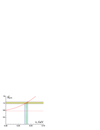
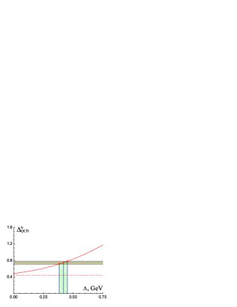
Figure 3: Juxtaposition of expression $\Delta^{\mbox{\tiny$\!\mbox{V/A}$}}_{\mbox{\tiny QCD}}$ (25) (solid curves) with relevant experimental data (10) (horizontal shaded bands). The solutions for QCD scale parameter $\Lambda$ are shown by vertical dashed bands.

The comparison of obtained result (25) with experimental data (10) gives nearly identical solutions for the QCD scale parameter $\Lambda$ in both channels, see Fig. 3. Namely, $\Lambda=(408\pm 30)\,$MeV for vector channel and $\Lambda=(418\pm 35)\,$MeV for axial–vector one. Additionally, both these values agree with the aforementioned perturbative solution for vector channel. It is worth mentioning also that the use of OPAL data on $\tau$ lepton hadronic decay [26] yields quite similar results [25].

5 Conclusions

The theoretical description of inclusive $\tau$ lepton hadronic decay is performed in the framework of Dispersive approach to QCD. The significance of effects due to hadronization is convincingly demonstrated. The approach on hand proves to be capable of describing experimental data on $\tau$ lepton hadronic decay in vector and axial–vector channels. The vicinity of values of QCD scale parameter obtained in both channels bears witness to the self–consistency of developed approach.

The author is grateful to D. Boito, P. Colangelo, M. Davier, F. De Fazio, A. Francis, and S. Menke for the stimulating discussions and useful comments. This work is supported by grant JINR-12-301-01.

References

• [1] R. Barate et al. [ALEPH Collaboration], Eur. Phys. J. C 4, 409 (1998); S. Schael et al. [ALEPH Collaboration], Phys. Rept. 421, 191 (2005).
• [2] M. Davier, A. Hocker, and Z. Zhang, Rev. Mod. Phys. 78, 1043 (2006); M. Davier, S. Descotes–Genon, A. Hocker, B. Malaescu, and Z. Zhang, Eur. Phys. J. C 56, 305 (2008).
• [3] J. Beringer et al. [Particle Data Group Collaboration], Phys. Rev. D 86, 010001 (2012).
• [4] E. Braaten, S. Narison, and A. Pich, Nucl. Phys. B 373, 581 (1992).
• [5] W.J. Marciano and A. Sirlin, Phys. Rev. Lett. 61, 1815 (1988); E. Braaten and C.S. Li, Phys. Rev. D 42, 3888 (1990).
• [6] S.L. Adler, Phys. Rev. D 10, 3714 (1974).
• [7] A.A. Pivovarov, Z. Phys. C 53, 461 (1992); F. Le Diberder and A. Pich, Phys. Lett. B 286, 147 (1992); 289, 165 (1992).
• [8] P.A. Baikov, K.G. Chetyrkin, and J.H. Kuhn, Phys. Rev. Lett. 101, 012002 (2008); 104, 132004 (2010); P.A. Baikov, K.G. Chetyrkin, J.H. Kuhn, and J. Rittinger, Phys. Lett. B 714, 62 (2012).
• [9] R.P. Feynman, Photon–hadron interactions, Reading, MA: Benjamin (1972) 282p.
• [10] A.V. Radyushkin, preprint JINR E2–82–159 (1982); JINR Rapid Commun. 78, 96 (1996); arXiv:hep-ph/9907228; N.V. Krasnikov and A.A. Pivovarov, Phys. Lett. B 116, 168 (1982).
• [11] A.V. Nesterenko and J. Papavassiliou, J. Phys. G 32, 1025 (2006); A.V. Nesterenko, SLAC eConf C0706044, 25 (2007); arXiv:0710.5878 [hep-ph].
• [12] A.V. Nesterenko, Nucl. Phys. B (Proc. Suppl.) 186, 207 (2009).
• [13] A.V. Nesterenko and J. Papavassiliou, Phys. Rev. D 71, 016009 (2005); Int. J. Mod. Phys. A 20, 4622 (2005); Nucl. Phys. B (Proc. Suppl.) 152, 47 (2005); 164, 304 (2007).
• [14] M. Della Morte, B. Jager, A. Juttner, and H. Wittig, JHEP 1203, 055 (2012).
• [15] M. Baldicchi, A.V. Nesterenko, G.M. Prosperi, and C. Simolo, Phys. Rev. D 77, 034013 (2008).
• [16] A.V. Nesterenko, Phys. Rev. D 62, 094028 (2000); 64, 116009 (2001).
• [17] A.V. Nesterenko, Int. J. Mod. Phys. A 18, 5475 (2003); Nucl. Phys. B (Proc. Suppl.) 133, 59 (2004); arXiv:hep-ph/0010257.
• [18] A.V. Nesterenko and C. Simolo, Comput. Phys. Commun.  181, 1769 (2010); 182, 2303 (2011).
• [19] D.V. Shirkov and I.L. Solovtsov, Phys. Rev. Lett. 79, 1209 (1997); Theor. Math. Phys. 150, 132 (2007); K.A. Milton and I.L. Solovtsov, Phys. Rev. D 55, 5295 (1997); 59, 107701 (1999).
• [20] K.A. Milton, I.L. Solovtsov, and O.P. Solovtsova, Mod. Phys. Lett. A 21, 1355 (2006); G. Cvetic, C. Valenzuela, and I. Schmidt, Nucl. Phys. B (Proc. Suppl.) 164, 308 (2007).
• [21] G. Cvetic and C. Valenzuela, Braz. J. Phys. 38, 371 (2008); A.P. Bakulev, Phys. Part. Nucl. 40, 715 (2009); G. Cvetic and A.V. Kotikov, J. Phys. G 39, 065005 (2012).
• [22] A.V. Nesterenko, SLAC eConf C1106064, 23 (2011); arXiv:1106.4006 [hep-ph].
• [23] A.I. Akhiezer and V.B. Berestetsky, Quantum electrodynamics, Interscience, NY (1965) 868p.
• [24] A.V. Nesterenko, arXiv:1110.3415 [hep-ph]; arXiv:1209.0164 [hep-ph].
• [25] A.V. Nesterenko, in preparation.
• [26] K. Ackerstaff et al. [OPAL Collaboration], Eur. Phys. J. C 7, 571 (1999); D. Boito, M. Golterman, M. Jamin, A. Mahdavi, K. Maltman, J. Osborne, and S. Peris, Phys. Rev. D 85, 093015 (2012).