Complex-valued information entropy measure
for networks with directed links (digraphs).
Application to citations by community agents with opposite opinions

Abstract

The notion of complex-valued information entropy measure is presented. It applies in particular to directed networks (digraphs). The corresponding statistical physics notions are outlined. The studied network, serving as a case study, in view of illustrating the discussion, concerns citations by agents belonging to two distinct communities which have markedly different opinions: the Neocreationist and Intelligent Design Proponents, on one hand, and the Darwinian Evolution Defenders, on the other hand.
The whole, intra- and inter-community adjacency matrices, resulting from quotations of published work by the community agents, are elaborated and eigenvalues calculated. Since eigenvalues can be complex numbers, the information entropy may become also complex-valued. It is calculated for the illustrating case.
The role of the imaginary part finiteness is discussed in particular and given some physical sense interpretation through local interaction range consideration. It is concluded that such generalizations are not only interesting and necessary for discussing directed networks, but also may give new insight into conceptual ideas about directed or other networks. Notes on extending the above to Tsallis entropy measure are found in an Appendix.

keywords : Entropy – Citation networks – Asymmetric adjacency matrix

1 Introduction

”Complicated systems” are usually, but abusively [1], called complex systems. Recall that complex numbers are found in physics to describe various macroscopic properties: the dielectric permittivity, the electric impedance, the amplitudes and phase angles of modal vibrations, Magnetic Resonance images, etc..

Complex eigenvalues (EVs) do $naturally$ occur in a Hamiltonian formalism: the imaginary part of some self-energy which turns out to be the ”density of states”, localization in superconductors [5], dissipation and scattering in Quantum Chaos [6, 7] or Quantum Chromodynamics, with a non-vanishing chemical potential [8], fractional Quantum Hall Effect [9], two-dimensional plasma of charged particles [10, 11]. See also the imaginary part of the ”free energy” measuring the quantum decay rate of a pure state or the imaginary part of power law exponents describing oscillations in the specific heat or in the electrical resistivity temperature derivative at (magnetic, for example) transitions [3, 4].

It will be argued below that one modern case of interest is the entropy of directed networks: it can have a real and an imaginary part. For coherence, the definitions of the thermodynamic and the information entropy measure are recalled in Sect. 2. Subsequently the complex information entropy measure (CIE) is defined in order to take into account complex algebra, when or if necessary, - in particular when discrete ”states” are considered. In Sect. 3, a brief outline of some illustrating case is presented. It concerns a citation network, - see Sect. 3.1. The entropy of such digraphs can be complex, following some illustrative calculation. A preliminary interpretation follows in Sect. 3.2.

Some conclusion is found in Sect. 4. A discussion on normalization is found in Appendix A. An extension to Tsallis entropy measure is suggested in Appendix B. A long but useful discussion on the origin of complex EV for citation and similar asymmetric networks is found in Appendix C, where the various cases of the most simple asymmetric networks, i.e. triads, described by 3x3 matrices, are used to point to transitivity causes.

2 Complex-valued information entropy measure

The typical statistical mechanics approach starts from the partition function $Z$ defined through the sum of all the Boltzmann factors measuring the probability of occurrence of the various states of a Hamiltonian $\cal H$. The partition function reads

$$Z_{s}(T)=\Sigma_{\nu=1}^{N_{s}}e^{-\beta\cal H(s,\nu)}.$$ (1)

when observing a system at a scale $s$ and at some temperature $T$ ($\beta\equiv 1/k_{B}T$); $\nu$ $(=1,...,N_{s})$ is an index allowing to label and to count the configurations of the relevant degrees of freedom governing the system. One can next derive the corresponding free energy $F_{s}(T)=-k_{B}T\;ln(Z_{s}(T))$. This free energy is known to be a homogeneous function at critical points [14], in the scaleless situation. This leads to define (real) critical exponents [15, 16]. The scale of interest is in fact related to the coherence length, $\xi$, itself temperature dependent, giving some measure of the ”temperature distance”, $\epsilon\equiv(T-T_{c})/T_{c}$, between the critical temperature $T_{c}$ and the system temperature $T$. Practically, one can map the model Hamiltonian $\cal H$ over the possible states, through $e^{-\beta\cal H}$. Without justifying much here, i.e. going back to the theory of Markov processes, we admit that the latter is a so called transfer matrix [17], with elements made of Boltzmann factors. Thereafter we can calculate the eigenvalues $\lambda_{i}$ and evaluate $Z$, $F$, and $S$, i.e. $e^{-\beta{\cal H}}$ $\rightarrow$ $e^{-\beta E}$ $\rightarrow$ $e^{-\beta\lambda_{i}}$ $\rightarrow$ $Z$ $\rightarrow$ $F$ $\rightarrow$ $\simeq$ $\lambda_{1}-k_{B}T\;ln\left(1+e^{-\beta(\lambda_{2}-\lambda_{1})}+...\right)$ $\rightarrow$ $S$. Often, the first eigenvalue $\lambda_{1}$ is sufficient to obtain an estimate of the free energy. So called ”corrections” imply higher order terms [18], though one often stops at $\lambda_{2}$. Thus, any (thermodynamic) property, $\chi(s,T)$, derived from $F_{s}(T)\sim F(\xi(\epsilon))$, can have the form $\chi(\epsilon)\sim\xi^{\tau}(\epsilon),$ but where $\tau$ can be complex [19, 20]. In some sense, this is as if $F$ is complex, or if some $\lambda_{i}$ is complex.

We interpret an adjacency matrix, e.g. describing a network, as a transfer matrix, - written in terms of some Hamiltonian $\cal H$. However, we are aware that such an $\cal H$ is not necessarily a bona fide Hamiltonian, i.e., from a quantum mechanics point of view, since it might not be hermitian. The eigenvalues can thus be complex.

2.1 Real algebra information entropy measure

The Boltzmann entropy in statistical physics  [12] reads:

$$S=-\int_{0}^{\infty}\mbox{d}wN(w,t)\log{N(w,t)}.$$ (2)

where $N(w,t)$ is the number of states, of type $w$, at time $t$. This entropy corresponds to the usual Shannon information entropy which can also be written in terms of the (equilibrium) probability $p_{i}$ of finding some (macroscopic variable in some) state $i$,

$$H=-k_{B}\sum_{i}p_{i}\ln p_{i}$$ (3)

Since $p_{i}$ is necessarily positive but less than 1, $H\geq 0$, - like a Boltzmann factor.

Often, $p_{i}$ is practically known through some a priori bin decompositionof the distribution of states. This is similar to the Theil approach in economy [21, 22, 23], where the individual incomes are taken into account, normalized to the income of the whole population of interest in the study. Thus, in the above, some generalization would replace $p_{i}$ by $\lambda_{i}$.

Having in mind applications to network theory, one might argue that the most adequate normalization should take into account the size of the system (or the adjacency matrix). In the Theil spirit, one could imagine various normalizations, see Appendix A. This can be considered elsewhere depending on specific applications.

Thereafter, the Information Entropy ($IE$) is defined, as in [24, 25], by

$$H=1+\sum\limits_{i=1}^{l_{M}}{\frac{{\lambda_{i}}}{{l_{M}}}\log_{l_{M}}\frac{{\lambda_{i}}}{{l_{M}}}}$$ (4)

in units where $k_{B}=1$, and where $\lambda_{i}$ is the i-th eigenvalue of the relevant matrix of size $l_{M}$ x $l_{M}$. However, one may, without much loss of generality, decide that the log-basis is the natural one, rather than one being associated with the matrix size, i.e. to keep a thermodynamic-like spirit, and redefine for our purpose,

$$H_{e}\equiv 1+\sum\limits_{i=1}^{l_{M}}{\frac{{\lambda_{i}}}{{l_{M}}}\ln\frac{{\lambda_{i}}}{{l_{M}}}}.$$ (5)

to emphasize that we the natural log. Nevertheless, for simplicity, the index _e will not be further written.

In concluding this section, let us introduce the notation $H_{1}\equiv 1+{\frac{{\lambda_{1}}}{{l_{M}}}\ln\frac{{\lambda_{1}}}{{l_{M}}}}.$ such that it should correspond to an estimate of the $IE$ based on the largest EV.

2.2 Complex information entropy measure

In fact, let $l_{M}$ is the number of available states, or the number of EVs for some Hamiltonian or transfer matrix or adjacency matrix. Since the $l_{M}$ eigenvalues could be complex, one has to generalize the previous formula, Eq. (5) to the complex plane, i.e. $H=H^{{}^{\prime}}+\;i\;H^{{}^{\prime\prime}}$, such as one gets

$$H^{{}^{\prime}}=1+\sum\limits_{i=1}^{l_{M}}\;\frac{{\|\lambda_{i}}\|}{{l_{M}}}\;\left([\ln\frac{{\|\lambda_{i}}\|}{{l_{M}}}][cos(\Phi_{i})]-[(\Phi_{i}+i\;n\;2\pi)\;sin(\Phi_{i})]\right),$$ (6)

and

$$H^{{}^{\prime\prime}}=\sum\limits_{i=1}^{l_{M}}\;\frac{{\|\lambda_{i}}\|}{{l_{M}}}\;\left([\ln\frac{{\|\lambda_{i}}\|}{{l_{M}}}][sin(\Phi_{i})]+[(\Phi_{i}+i\;n\;2\pi)\;cos(\Phi_{i})]\right),$$ (7)

where we identify any $\lambda_{i}^{{}^{\prime}}+i\;\lambda_{i}^{{}^{\prime\prime}}$ with $\|\lambda_{i}\|\;[cos(\Phi_{i})+i\;sin(\Phi_{i})]$. Note that from these, the magnitude $\|H\|$ of the complex information entropy, as well as the $IE$ phase factor, could be calculated. The $i\;n\;2\pi$ term is due to the fact that the argument of log $\lambda_{i}$ is a multivalued function [2]. Therefore, for meaningfully pursuing any calculation, it is necessary to define the existence interval of the argument of such a complex number. One can decide that $\Phi_{i}$ is defined in $0\leq\;\Phi_{i}\;<+2\pi$, or in $-\pi<\;\Phi_{i}\;\leq\;+\pi$, i.e. the so called ”principal value” (PV) component [2].

Thus, when doing the summations in Eq.(6) and Eq.(7), several terms may cancel each other. In particular, when either $\Phi_{i}\;tan(\Phi_{i})$ is even or when $\Phi_{i}\;cotan(\Phi_{i})$ is odd. This depends on whether two EVs are complex conjugates, and in the appropriately defined space of $\Phi_{i}$. Then, the above formulae can be simplified through some trivial algebra when taking into account the form of the eigenvalue.

Whence, starting from Eq.(5), let us distinguish between the real positive ($\rho$), real negative ($\nu$), imaginary ($\mu$), equal to zero, and complex-valued ($\lambda)$ eigenvalues. One can rewrite Eq.(7), with obvious notations for each sum upper limit,

$$H=1+\sum\limits_{i=1}^{\rho_{M}}\frac{\rho_{i}}{l_{M}}\ln\frac{\rho_{i}}{l_{M}}+\sum\limits_{i=1}^{\nu_{M}}\frac{\nu_{i}}{l_{M}}\ln\frac{\nu_{i}}{l_{M}}+\sum\limits_{i=1}^{\mu_{M}}\frac{\mu_{i}}{l_{M}}\ln\frac{\mu_{i}}{l_{M}}+\sum\limits_{i=1}^{\lambda_{M}}\frac{\lambda_{i}}{l_{M}}\ln\frac{\lambda_{i}}{l_{M}}\;.$$ (8)

The first sum is trivially real, for any interval definition of $\Phi_{i}$. In fact, $\rho_{i}=\|\rho_{i}\|$.

When an EV has some finite, in particular if it is negative, real or imaginary part, several cases must be distinguished. The case of degenerate EVs has also to be specially considered. Note that if an EV is evenly degenerate, it can be considered as stemming from a set of $c.c.$ EV with a zero imaginary part. Then, $\frac{\lambda_{i}}{l_{M}}\ln\frac{\lambda_{i}}{l_{M}}$ depends on which complex sheet (”interval space”) the phase factor is defined.

2.2.1 $\Phi_{i}$ $\in$ [0, 2$\pi$[ space

• When $\nu_{i}^{{}^{\prime}}$ = -$\|\nu_{i}^{{}^{\prime}}\|$, and $\nu_{i}^{{}^{\prime\prime}}=0$, one has $\nu_{i}\equiv\|\nu_{i}^{{}^{\prime}}\|\;e^{i\pi+2ni\pi}$; the second summation has thus terms like ${\frac{{\nu_{i}}}{{l_{M}}}\ln\frac{{\nu_{i}}}{{l_{M}}}}$ $\equiv$ $-\frac{\|\nu_{i}^{{}^{\prime}}\|}{l_{M}}\;\left[ln[\frac{\|\nu_{i}^{{}^{\prime}}\|}{{l_{M}}}]+(2n+1)i\;[\pi]\right]$. Such a term contains a real $and$ an imaginary part. The $n=0$ case is of course in order here below, i.e. ${\frac{{\nu_{i}}}{{l_{M}}}\ln\frac{{\nu_{i}}}{{l_{M}}}}$ $\equiv$ $-\frac{\|\nu_{i}^{{}^{\prime}}\|}{l_{M}}\;ln[\frac{\|\nu_{i}^{{}^{\prime}}\|}{{l_{M}}}]-\frac{\|\nu_{i}^{{}^{\prime}}\|}{l_{M}}i\;[\pi]$.

• In the third summation, the imaginary part $\mu_{i}^{{}^{\prime\prime}}$ could be positive or negative, i.e. $\mu_{i}\equiv i\;\mu_{i}^{{}^{\prime\prime}}=\pm i\|\mu_{i}\|$; the phase factor is $\left[\frac{\pi}{2}\right]$ and $\left[\frac{3\pi}{2}\right]$, respectively. Thus, a term in the third summation reads either

  $+i\frac{\|\mu_{i}\|}{l_{M}}\;\left[ln(\frac{\|\mu_{i}\|}{l_{M}})+i[\frac{\pi}{2}]\right]$$\equiv-[\frac{\pi}{2}]\frac{\|\mu_{i}\|}{l_{M}}\;+i\frac{\|\mu_{i}\|}{l_{M}}\;ln(\frac{\|\mu_{i}\|}{l_{M}})$,

  or $-i\frac{\|\mu_{i}\|}{l_{M}}\;\left[ln(\frac{\|\mu_{i}\|}{l_{M}})+i[\frac{3\pi}{2}]\right]$$\equiv[\frac{3\pi}{2}]\frac{\|\mu_{i}\|}{l_{M}}\;$ $-i\frac{\|\mu_{i}\|}{l_{M}}\;ln(\frac{\|\mu_{i}\|}{l_{M}})$.

  Therefore, in the summation, extending over the whole number ($\mu_{M}$) of imaginary, - but necessarily ($c.c.$), EVs, we insist, only a $real$ term subsists in $H$ after summing over $c.c.$ EVs, i.e. $+\|\mu_{i}\|\;\pi/l_{M}$. Note the + sign.

• Let $\lambda_{i}^{{}^{\prime}}+i\;\lambda_{i}^{{}^{\prime\prime}}\equiv\|\lambda_{i}\|\;[cos(\Phi_{i})+i\;sin(\Phi_{i})]\equiv\|\lambda_{i}\|\;e^{+i\Phi_{i}}$. Thus, $\lambda_{i}^{{}^{\prime}}-i\;\lambda_{i}^{{}^{\prime\prime}}\equiv\|\lambda_{i}\|\;[cos(\Phi_{i})-i\;sin(\Phi_{i})]\equiv\|\lambda_{i}\|\;e^{+i(2\pi-\Phi_{i})}$. One has,

  $\frac{\|\lambda_{i}\|}{l_{M}}\;ln\frac{\|\lambda_{i}\|}{l_{M}}\equiv\;\frac{\|\lambda_{i}\|}{l_{M}}\left[cos(\Phi_{i})\;ln\frac{\|\lambda_{i}\|}{l_{M}}-\Phi_{i}\;sin(\Phi_{i})\right]$
    $+\;\;i\;\;\frac{\|\lambda_{i}\|}{l_{M}}\;\left[\Phi_{i}\;cos(\Phi_{i})+ln\frac{\|\lambda_{i}\|}{l_{M}}sin(\Phi_{i})\right],$… if $\lambda\equiv\lambda_{i}^{{}^{\prime}}+i\;\lambda_{i}^{{}^{\prime\prime}}$.

  But when $\lambda\equiv\lambda_{i}^{{}^{\prime}}-i\;\lambda_{i}^{{}^{\prime\prime}}$, one has $\frac{\|\lambda_{i}\|}{l_{M}}\;ln\frac{\|\lambda_{i}\|}{l_{M}}$
  $\equiv\;\frac{\|\lambda_{i}\|}{l_{M}}\;.\left[cos(\Phi_{i})\;ln\frac{\|\lambda_{i}\|}{l_{M}}+(2\pi-\Phi_{i})\;sin(\Phi_{i})\right]$

  +$i$ $\frac{\|\lambda_{i}\|}{l_{M}}\left[(2\pi-\Phi_{i})\;cos(\Phi_{i})-ln\frac{\|\lambda_{i}\|}{l_{M}}\;sin(\Phi_{i})\right].$ Therefore, the fourth summation can be simplified; after grouping $c.c.$ terms, as indicated by the notation $\sum^{{}^{\prime}}_{i}$, it reads

  $\sum^{{}^{\prime}}_{i}$ $2\frac{\|\lambda_{i}\|}{l_{M}}\left[cos(\Phi_{i})\;ln\frac{\|\lambda_{i}\|}{l_{M}}+(\pi-\Phi_{i})sin(\Phi_{i})\right]+$
  $+i$ $\sum^{{}^{\prime}}_{i}\;2\pi\frac{\|\lambda_{i}\|}{l_{M}}cos(\Phi_{i})$.

One can rewrite the real and imaginary parts of the $IE$ such that,

$$\phantom{}H^{{}^{\prime}}_{TC}=1+\sum\limits_{i=1}^{\rho_{M}}\;\frac{{\|\rho_{i}}\|}{{l_{M}}}\;\left[\ln(\frac{{\|\rho_{i}}\|}{{l_{M}}})\right]+$$

$$\sum\limits_{i=1}^{\nu_{M}}\;\frac{-\|\nu_{i}\|}{l_{M}}\;\left[\ln(\frac{{\|\nu_{i}}\|}{{l_{M}}})\right]+$$

$$\sum_{i}^{{}^{\prime}}\;\frac{\|\mu_{i}\|}{l_{M}}\;\left[\pi\right]+$$

$$2\;\sum_{i}^{{}^{\prime}}\left[\frac{\lambda_{i}^{{}^{\prime}}}{l_{M}}\ln(\frac{{\|\lambda_{i}}\|}{{l_{M}}})+(\pi-\Phi_{i})\frac{\lambda_{i}^{{}^{\prime\prime}}}{l_{M}}\right]$$ (9)

and

$$H^{{}^{\prime\prime}}_{TC}=\sum\limits_{i=1}^{\nu_{M}}\;\left[\frac{-\|\nu_{i}\|\;\pi}{l_{M}}\;\right]+\sum^{{}^{\prime}}_{i}\;2\pi\frac{\|\lambda_{i}\|}{l_{M}}cos(\Phi_{i}).$$ (10)

2.2.2 Principal Value (PV) space : $\Phi_{i}$ $\in$ ]-$\pi,\pi$]

• When $\nu_{i}^{{}^{\prime}}$ = -$\|\nu_{i}^{{}^{\prime}}\|$, and $\nu_{i}^{{}^{\prime\prime}}=0$, one can obtain, as in TC space, ${\frac{{\nu_{i}}}{{l_{M}}}\ln\frac{{\nu_{i}}}{{l_{M}}}}$ $\equiv$ $-\frac{\|\nu_{i}^{{}^{\prime}}\|}{l_{M}}\;ln[\frac{\|\nu_{i}^{{}^{\prime}}\|}{{l_{M}}}]-\frac{\|\nu_{i}^{{}^{\prime}}\|}{l_{M}}i\;[\pi]$.

• Recall that in the third summation, the imaginary part $\mu_{i}^{{}^{\prime\prime}}$ could be positive or negative, i.e. $\mu_{i}\equiv i\;\mu_{i}^{{}^{\prime\prime}}=\pm i\|\mu_{i}\|$. In PV space, the phase factor is $\left[\frac{\pi}{2}\right]$ and $\left[-\frac{\pi}{2}\right]$, respectively. Thus, a term in the third summation reads either $+i\frac{\|\mu_{i}\|}{l_{M}}\;\left[ln(\frac{\|\mu_{i}\|}{l_{M}})+i[\frac{\pi}{2}]\right]$ or $-i\frac{\|\mu_{i}\|}{l_{M}}\;\left[ln(\frac{\|\mu_{i}\|}{l_{M}})-i[\frac{\pi}{2}]\right]$.

  Therefore, in the summation, extending over the whole number ($\mu_{M}$) of imaginary, - but necessarily $c.c.$ EVs, we again insist, only a $real$ term subsists in $H$ after summing over $c.c.$ EVs, i.e. $-\|\mu_{i}\|\;\pi/l_{M}$. Note the $-$ sign.

• Because $\lambda_{i}^{{}^{\prime}}\pm i\;\lambda_{i}^{{}^{\prime\prime}}\equiv\|\lambda_{i}\|\;[cos(\Phi_{i})\pm i\;sin(\Phi_{i})]\equiv\|\lambda_{i}\|\;e^{\pm i\Phi_{i}}$, terms like $\frac{\|\lambda_{i}\|}{l_{M}}\;ln\frac{\|\lambda_{i}\|}{l_{M}}\equiv\;$
  $\frac{\|\lambda_{i}\|}{l_{M}}\left[[cos(\Phi_{i})\;ln\frac{\|\lambda_{i}\|}{l_{M}}-\Phi_{i}\;sin(\Phi_{i})]\pm\;i[\Phi_{i}cos(\Phi_{i})+sin(\Phi_{i})\;ln\frac{\|\lambda_{i}\|}{l_{M}}]\right]$.

  Taking into account that the $\lambda$ EVs are necessarily $c.c.$, the fourth summation can be simplified into a real quantity, after grouping $c.c.$ terms, as indicated by $\sum^{{}^{\prime}}_{i}$, i.e.

  $\sum_{i}^{{}^{\prime}}$ $2\left[\frac{\lambda_{i}^{{}^{\prime}}}{l_{M}}\;ln\frac{\|\lambda_{i}\|}{l_{M}}-\Phi_{i}\;\frac{\lambda_{i}^{{}^{\prime\prime}}}{l_{M}}\right]$ which also reads

  $\sum^{{}^{\prime}}_{i}$ $2\frac{\|\lambda_{i}\|}{l_{M}}\left[cos(\Phi_{i})\;ln\frac{\|\lambda_{i}\|}{l_{M}}-\Phi_{i}sin(\Phi_{i})\right]$.

One can regroup the real and imaginary parts such that finally,

$$\phantom{}H^{{}^{\prime}}_{PV}=1+\sum\limits_{i=1}^{\rho_{M}}\;\frac{{\|\rho_{i}}\|}{{l_{M}}}\;\left[\ln(\frac{{\|\rho_{i}}\|}{{l_{M}}})\right]+$$

$$\sum\limits_{i=1}^{\nu_{M}}\;\frac{-\|\nu_{i}\|}{l_{M}}\;\left[\ln(\frac{{\|\nu_{i}}\|}{{l_{M}}})\right]+$$

$$\sum_{i}^{{}^{\prime}}\;-\frac{\|\mu_{i}\|}{l_{M}}\;\left[\pi\right]+$$

$$2\;\sum^{{}^{\prime}}_{i}\left[\frac{\lambda_{i}^{{}^{\prime}}}{l_{M}}\ln(\frac{{\|\lambda_{i}}\|}{{l_{M}}})-\Phi_{i}\frac{\lambda_{i}^{{}^{\prime\prime}}}{l_{M}}\right]$$ (11)

and

$$H^{{}^{\prime\prime}}_{PV}=\sum\limits_{i=1}^{\nu_{M}}\;\left[\frac{-\|\nu_{i}\|\;\pi}{l_{M}}\;\right].$$ (12)

It can be observed that $H^{{}^{\prime}}_{PV}$ can have any sign. However, $H^{{}^{\prime\prime}}_{PV}$ is necessarily $\leq 0$. Moreover, if the EV of type $\nu$ is evenly degenerate, it has to be recognized that such EVs are equivalent to a $c.c.$ EV, with zero imaginary part. Thus, ${\frac{{\nu_{i}}}{{l_{M}}}\ln\frac{{\nu_{i}}}{{l_{M}}}}$ $\equiv$ $-\frac{\|\nu_{i}^{{}^{\prime}}\|}{l_{M}}\;ln[\frac{\|\nu_{i}^{{}^{\prime}}\|}{{l_{M}}}]\pm\frac{\|\nu_{i}^{{}^{\prime}}\|}{l_{M}}i\;[\pi]$. Therefore, the summation over such degenerate EVs is equal to $-2\;\frac{\|\nu_{i}^{{}^{\prime}}\|}{l_{M}}\;ln[\frac{\|\nu_{i}^{{}^{\prime}}\|}{l_{M}}]$ and leads to a zero imaginary part contribution.

Note also that if the Principal Value (PV) space is rather the PV’ space such that $\Phi_{i}$ $\in$ [-$\pi,\pi$[, one would obtain ${\frac{{\nu_{i}}}{{l_{M}}}\ln\frac{{\nu_{i}}}{{l_{M}}}}$ $\equiv$ $-\frac{\|\nu_{i}^{{}^{\prime}}\|}{l_{M}}\;ln[\frac{\|\nu_{i}^{{}^{\prime}}\|}{{l_{M}}}]+i\;[\pi]\;\frac{\|\nu_{i}^{{}^{\prime}}\|}{l_{M}}$, instead. Appropriate modifications would have to occur when writing $H^{{}^{\prime}}_{PV^{\prime}}$ and $H^{{}^{\prime\prime}}_{PV^{\prime}}$. Yet, the contribution of evenly degenerate negative EVs would still lead to a vanishing contribution to $H^{{}^{\prime\prime}}_{PV^{\prime}}$.

To verify the above formulae and conclusions, it can be also usefully checked that the $\nu$ and $\mu$ cases can be obtained as special cases of the $\lambda$ case.

3 Data

Let us consider a numerical example covering various cases among complex (= complicated) networks.These have been used to depict the characteristics of various abstract systems. The network nodes can be motifs or agents, while the links can be directed or undirected, weighted or not.

Among directed networks [26, 27, 28, 29, 30, 31, 32, 33, 34, 35, 36, 37, 38, 39], a special class is the citation networks [40, 41, 42, 43], which is called a digraph. Digraphs are surveyed in [44].

Due to the intrinsically time dependent hierarchical process, the adjacency matrix representing the network is usually asymmetric, beside being a non-negative matrix. There is a large body of mathematical work on spectra of adjacency matrices, ranging from modern versions of Perron-Frobenius theorem for non-negative matrices [45, 46], - up to recent results reviewed by Brualdi [47] and others like [48, 49, 50, 51, 52, 53].

For the following, let it be recalled that a square matrix $\cal M$ is so called irreducible if $D(\cal M)$, the corresponding network is strongly connected, i.e. a path exists between any couple of nodes. Otherwise $\cal M$ is said to be reducible. Let $\cal M$ $\geq$ 0 be an irreducible $n$ x $n$ matrix. Then, $\cal M$ has a positive real eigenvalue equal to its spectral radius $\rho(\cal M).$ An irreducible nonnegative matrix $\cal M$ is said to be primitive, if the only eigenvalue of $\cal M$ of modulus $\rho(\cal M)$ is $\rho(\cal M).$ An irreducible nonnegative matrix $\cal M$ is said to be cyclic of index $k$ $>$ 1, if it has $k$ eigenvalues of modulus equal to $\rho(\cal M).$

To illustrate the arguments leading to the CIE theory, we have therefore selected a citation network, previously studied along other lines [42, 43], but presenting a set of adjacency matrices containing quite a variety of features, in particular with respect to the EV distributions.

It might be useful to the reader to consider the case of the smallest asymmetric adjacency matrix, with zero on the diagonal for reasons given below, discussed in Appendix C. Even though it might look surprising to discuss a 3x3 matrix in a modern scientific paper, the illustrations found in the Appendix have been found to be the most simple ones leading to the appreciation of the EV behavior of large random matrices. Indeed such matrices correspond to complicated networks from which it is not often possible to easily observe the key features.

3.1 A 77x77 real asymmetric matrix

Consider the citation network first studied in [42], with adjacency matrices given in [43], according to the outcome from a Scholar Google search process. The citations are those of agents belonging to two quite distinct communities, composed of modern creationists (most are Intelligent Design (ID) proponents (IDP), on one hand, and Darwin’s theory of Evolution Defenders (DED), on the other hand. The network [43] is composed of two subgraphs, one with 37 and the other with 40 elements, or nodes, or agents, corresponding to the IDP and DED community, respectively. The adjacency matrices can be summarized as

$$M_{0}\equiv\left(\begin{tabular}[]{ll}$C_{0}$&$A$\\ $B$&$D_{0}$\end{tabular}\right)\;\equiv\left(\begin{tabular}[]{ll}$C_{0}$&$0$\\ $0$&$D_{0}$\end{tabular}\right)+\left(\begin{tabular}[]{ll}0&$A$\\ $B$&$0$\end{tabular}\right).$$ (13)

in which a matrix element $m_{ij}$ takes the value 1 or 0 depending on whether or not a citation of $i$ by $j$ has taken place, as recorded and explained in ref. [42, 43]. The matrices $C_{0}$ (37x37) and $D_{0}$ (40x40) indicate whether agents of community $i$ have been quoted by others of the same community $i$. In contrast, $F_{0}$, i.e.

$$F_{0}=\left(\begin{tabular}[]{ll}0&$A$\\ $B$&$0$\end{tabular}\right).$$ (14)

emphasizes links $between$ different communities, i.e. agents of community $j$ quoting those of community $i(\neq j)$; $i\leftarrow j$. $A$ and $B$ are obviously $rectangular$ matrices describing inter-community links. We emphasize with the ₀ index that all diagonal terms in $M_{0}$, $C_{0}$, and $D_{0}$ are $0$, i.e. we are $not$ considering any self-citation, i.e. $m_{ii}=0$. In brief, there are 91, 71, and 119 links, in IDP, DED and inter-community ones, respectively. All adjacency matrices, as well as $M_{0}$ and $F_{0}$ are markedly asymmetric and contain only real and positive numbers, 0 or 1; see [43] for the list of all finite matrix elements.

Moreover, since each square matrix $M_{0}$, $C_{0}$, $D_{0}$, $F_{0}$ has non-negative elements, the Perron-Frobenius theorem, see above, states that there exists a non negative eigenvalue greater or equal in absolute value than all other eigenvalues (and its corresponding eigenvector has non-negative components) [54, 55].

We have tested the hypothesis of irreducibility of these matrices. Since the property of irreducibility is equivalent to the property of the adjacency matrix corresponding to a strongly connected network, we have tested the irreducibility through the algorithm of Tarjan [56] It occurs that each matrix is reducible (i.e. not irreducible). In fact, beside a giant strongly connected component, there are many other (even $single$) units that stand alone as if strongly connected components for its neighborhood. This is due to the fact that the ”sample” reports authors that either only quote or are only quoted. Therefore, reversal links are missing, increasing thereby the number of strongly connected components. Therefore, extensions of the Perron-Frobenius theorem to irreducible matrices cannot be applied since each matrix $M_{0}$, $C_{0}$, $D_{0}$, $F_{0}$ reducible.

Of course, the Perron-Frobenius theorem for irreducible matrices could be applied on each single strongly connected component, - locally, w mean. However, it seems that this would give a (too) local result on the eigenvalue for all the short dimension sub-matrices. We have considered that it would not be useful for the present purpose, - nor to the global task of understanding the relevance of authors, - since the property of irreducibility is only interesting, in our opinion, for considering the strongly connected components. However, the strongly connected components may help in understanding the existence of ”hubs”, clusters and clubs, - if such is a question. Therefore, the Perron-Frobenius theorem, applied in its version for non-negative matrices only, indicates that there may exist eigenvalues of the same absolute value as the maximal one; moreover the maximal eigenvalue may not be a simple root of the characteristic polynomial, can be zero (and the corresponding eigenvector does not need to be strictly positive).

The EVs of the above 4 matrices, $M_{0}$, $C_{0}$, $D_{0}$, and $F_{0}$, have been computed. The EVs of interest are given in Tables 1-3. Some information ”summarizing” the structure of the EVs distribution is given in Table 5. The values of the CIE are also given in Table 4, from which the real part, imaginary part, absolute value and phase factor of $H$ could be deduced depending on the defining Riemann sheet.

3.2 Discussion

First, note some apparent similarity between the characteristics of the whole network and of the two subnetworks from Table 4. The ratios between the number of directed (DL), undirected (UL) or total number (L) of links are rather similar, - the DL/L ratio being a little bit larger for $C_{0}$.

Moreover, each largest EV is real and positive. The second largest EV can be either positive, like in $M_{0}$ and $D_{0}$, or complex, like in $C_{0}$ and $F_{0}$.

Recall that the real part of the main eigenvalue of an adjacency matrix is usually considered to be a measure of centrality of some node, like a leading agent. What is new here concerns the imaginary part which, as we consider, indicates the relative (inverse) scale or range of influence of such a leader.

The information entropy, deduced from the calculated EVs, enhances some difference between the networks, going beyond consideration on the ”main node”, or ”state” in a thermodynamic language. The real and imaginary parts of information entropy values for the matrices are presented in Table 4. First, one notes that $H_{1}$ values are all of the same order of magnitude. Next, it is apparent that $\|H\|$ are quasi similar whatever the used Riemann sheet, but more interestingly that the $M_{0}$ and $D_{0}$ values differ from those of $C_{0}$ and $F_{0}$. Yet, the $D_{0}$ $\|H\|$ value is very small and quasi equal to 0, in using the PV space.

$H^{{}^{\prime}}$ is markedly different for $C_{0}$ and for the other matrices. In fact, the real part of the IDP network $entropy$ $H$ is the only one to be positive, - but small. The other real parts are negative, in both spaces. In all cases, $H^{{}^{\prime\prime}}$ is negative.

Recall that the size of the matrices has been taken into account through the $l_{M}$ factor in the EV normalization.

Rather than spending more time on the numerical values, it seems more useful to stress the origin of such a complex information entropy as arising through the network structure. The key feature appears to be the ensemble of so called simple transitivity paths, as illustrated in App. C on small networks. This observation might also help in future deep mathematical work in order to sort out the property of EV distributions of random matrices. In fine, the complex part of the entropy truly emphasizes the delay in information, the citation sequence, and range of information, the connected nodes. In so doing, it seems that the CIE has brought a vision of directed networks different from other measures and other previous discussions, like one in [57], but considering acyclic networks.

4 Conclusions

Directed networks are very common. Citation networks belong to a huge subclass of those. It is common knowledge also that opinion formation demands information exchanges which are thereby necessarily ”directed” between agents. When representing such networks through adjacency matrices, it is apparent that such matrices are necessarily asymmetric.

This paper, on one hand, introduces a technique in order to obtain some insight into directed networks. It appears that one can consider a network information entropy through the link distribution on which information is exchanged. Through an analogy with Boltzmann entropy in usual statistical mechanics, one can observe that in order to get more insight on the network entropy, one can calculate the whole set of eigenvalues of the adjacency matrix of the network. This is similar to consider the set of discrete values of a transfer matrix in quantum or statistical mechanics. However, the resulting information entropy turns out to be a complex mathematical feature. It needs some interpretation. The latter can be based on the free energy concept.

Starting form the notion of equilibrium free energy, Zweger [58] attempted a dynamical interpretation of a classical complex free energy, in 1985. He pointed out that the problem is to determine a characteristic ”relaxation” time for some process in which the dynamical (Langevin or Fokker-Planck) equation is connected to some Hamiltonian or some corresponding transfer matrix. A probability current can be written, in fact, in terms of some unstable mode times an equilibrium factor which is the imaginary part of the free energy [59]. Usually [58, 60], the imaginary part of the free energy (or largest eigenvalues) give some information about the ”nucleation stage” of the dynamics. The real part, of course, determines the equilibrium energy state.

We propose that another, though related approach, can be considered. Instead of some ”relaxation time”, one may consider the ”spatial aspect of the phenomenon”, e.g. through some correlation range length $\xi$. This approach makes some sense,in particular for networks, analytically described through some Hamiltonian or transfer matrix. Moreover, such a spatial scale introduction may remind of some analogy with Discrete Scale Invariance (DSI) (or lack of DSI) feature [19, 20]. In fact, this DSI leads to complex dimensions and complex critical exponents.

The illustrating example implies two distinct communities, with markedly different opinions : the Neocreationist and Intelligent Design Proponents (IDP) on one hand, and the Darwinian Evolution Defenders (DED) on the other hand. These are communities for which an opinion consensus can be hardly expected. It appears that for the whole set of agents, two agents (”states”) are markedly dominating. They seem to belong to the DED community. In contrast, the IDP community has only one main ”state”. Interestingly, the same is true for the inter-community ” information exchange phenomenon” for which there is only one main dominating state.

In summary, we have presented an original work extension of $IE$, connecting the CIE method, to sound statistical mechanics. By examining, different eigenvalues of asymmetric matrices, - sometimes complex eigenvalues, yet starting with the largest ones, one can describe an $IE$, - like if in thermodynamics, one describes a free energy in terms of eigenvalues of some Hamiltonian. Thus, one not only obtains the ”basic” free energy, but also corrections due to some underlying scale structure. Moreover considerations on the mathematical form of the $IE$, i.e. its real and imaginary part, when they exist, allow to emphasize characteristics, which we attribute to the leadership range. This has been exemplified by considering a network with two specific communities having different opinions, exchanged through citations.

Note added at the completion of this report: Another argument in favor of studying asymmetric matrices can be mentioned. Indeed, during the process of finishing up the present work, for submission, a paper, submitted to to EPJB, occurred on arXives [61] entitled Asymmetric correlation matrices: an analysis of financial data. Due to the asymmetry in time delayed correlations between financial time series, it is indeed also of interest to extend the spectral analysis to the realm of complex eigenvalues, - as first attempted in [62]. Though different in essence, such works and the present one indicate that one should not be stacked to studying only systems within real algebra.

Acknowledgements

GR thanks the COST Action MP0801 for the STSM 4475 grant, allowing her stay at the University of Liege in Feb. 09. MA thanks the COST Action MP0801 for the STSM 6698 grant, allowing his stay at the University of Viterbo, in Sept. 2010.

Appendix A. Normalization considerations

In the main text, the Theil index form [22]

$$\frac{{\lambda_{i}}}{{<\lambda_{i}>}}\sum\limits_{i=1}^{l_{M}}\;\frac{{\lambda_{i}}}{{<\lambda_{i}>}},$$ (15)

has been adapted from its original writing, with real numbers, to one involving complex numbers, but the more so better appropriate for the $IE$, i.e.,

$$\frac{{\lambda_{i}}}{{l_{M}}}\sum\limits_{i=1}^{l_{M}}\;\frac{{\lambda_{i}}}{{l_{M}}},$$ (16)

with the ”normalization” $l_{M}$. Indeed, it would have been inappropriate to use the Theil index original normalization, since $<\lambda_{i}>=0$, because $\sum\limits_{i=1}^{l_{M}}\;\lambda_{i}=0$.

Appendix B. Tsallis entropy

Tsallis [63, 64, 65] proposed that a large category of systems may be treated by a similar formalism, but where a more general entropy measure is defined by

$$S_{q}=k_{B}\frac{(1-\sum_{i}p_{i}^{q})}{q-1}$$ (17)

which depends on the real parameter $q$ and which reduces to the Shannon entropy for $q\rightarrow$1. Along the lines in the main text, it is tempting to define a ${}_{q}IE$ as

$$H_{q}\equiv\;1+\;\frac{k_{B}}{q-1}(1-\sum_{i}p_{i}^{q})\equiv\;1+\frac{k_{B}}{q-1}\left(1-\sum_{i}[\frac{\lambda_{i}}{l_{M}}]^{q}\right)$$ (18)

thereby accepting a complex-valued $IE$ in Tsallis sense.

Tsallis theory is sometimes referred to in the literature as no-extensive statistical mechanics, in contrast with the extensivity of the Shannon entropy. For general $q$, a proper extremisation of Eq.(17) leads to generalized canonical distributions, often called Tsallis distributions,

$$f_{q}(x)=\frac{e_{q}^{-\beta^{{}^{\prime}}x}}{Z_{s}(q)}$$ (19)

where $x$ denotes the energy of the system, $Z_{s}(q)\equiv\Sigma_{\nu=1}^{N_{s}}e^{-{\cal H}(s,\nu)^{q}}$, and $e_{q}^{x}$ is the $q$-exponential function defined by

$$e_{q}^{x}\equiv(1+(1-q)x)^{\frac{1}{1-q}}.$$ (20)

One should also note that Tsallis formalism draws a direct parallelism with the equilibrium theory, where $\beta^{{}^{\prime}}$ plays the role of the inverse of a temperature, and $Z$ that of a partition function. However Tsallis and others [63, 64, 65] have often insisted ion the connexion between $q$- and non-equilibrium effects. One might consider connecting the above $IE$ to Tsallis considerations, in further work; see already [66]. Recall that a $q-$Theil index has been already introduced [67, 68].

Appendix C. A 3x3 matrix

Let a state Hamiltonian be described by a 3x3 matrix

$$\cal H=\left(\begin{tabular}[]{llll}$H_{11}$&$H_{12}$&$H_{13}$\\ $H_{21}$&$H_{22}$&$H_{23}$\\ $H_{13}$&$H_{23}$&$H_{33}$\end{tabular}\right)\;.$$ (21)

To remain within a ”no self-citation” scheme, let all the diagonal elements be equal to zero, i.e. $H_{11}=H_{22}=H_{33}$ = 0, and call this ”new” matrix ${\cal H}_{0}$. Moreover, let all non diagonal elements be equal to either 1 or 0. These ”reductions” are made in the spirit of tying the present subsection to the main text, involving a (”large”) citation network for which the (adjacency) matrix has elements taking only a 1 or 0 value.

Recall that the EVs of any 3x3 matrix are solutions of the cubic equation

$$-\lambda^{3}+\lambda^{2}\;tr({\cal H}_{0})+\frac{\lambda}{2}[tr({\cal H}_{0})^{2}-tr^{2}({\cal H}_{0})]+det({\cal H}_{0})=0.$$ (22)

By ”construction”, $tr(\cal H$${}_{0})=tr^{2}(\cal H$${}_{0})=0.$ Moreover, one easily obtains that $tr(\cal H$${}_{0})^{2}/2=H_{12}H_{21}+H_{13}H_{31}+H_{23}H_{32}$, and $det(\cal H$${}_{0})=H_{13}H_{32}H_{21}+H_{31}H_{12}H_{23}$. Therefore, only 7 types of cubic equations, as Eq.(22), have to be considered

• type I  : $-\lambda^{3}+3\lambda+2=0$

• type II  : $-\lambda^{3}+2\lambda+1=0$

• type III : $-\lambda^{3}+\lambda+1=0$

• type IV : $-\lambda^{3}+\lambda+0=0$

• type V  : $-\lambda^{3}+2\lambda+0=0$

• type VI : $-\lambda^{3}+0\lambda+1=0$

• type VII : $-\lambda^{3}+0\lambda+0=0$

It is somewhat easily deduced that only type III and type VI lead to complex eigenvalues. Both types have one positive real root. Note that the type I cubic equation has a real negative (of course evenly) degenerate root = -1, requesting special attention when calculating $H$; see end of Sect. 2.2.

The networks made of three nodes corresponding to such cubic equations are illustrated in Fig. 5, - one network is displayed for each case only; the others are easily and readily deduced by permutation of bonds [69, 70, 71]. On one hand, this illustrates well why type I has degenerate eigenvalues. On the other hand, the complex eigenvalues (type III and type VI) are now understood as arising from the transitivity relationship, corresponding to 14-120C and 9-030T triads, in Pajek Manual notations [72].

Even though it might look surprising to describe 3x3 matrices in a modern scientific paper, the present illustration has been found necessary as the most simple one leading to some appreciation of the EV behavior of larger random matrices.

Figure 1: Distribution of the eigenvalues (EVs) of the matrix $M_{0}$ in the complex plane

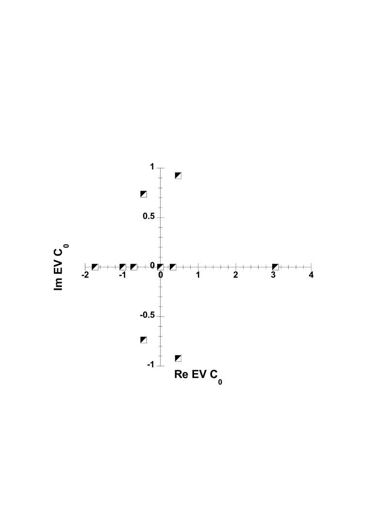
Figure 2: Distribution of the eigenvalues (EVs) of the matrix $C_{0}$ in the complex plane

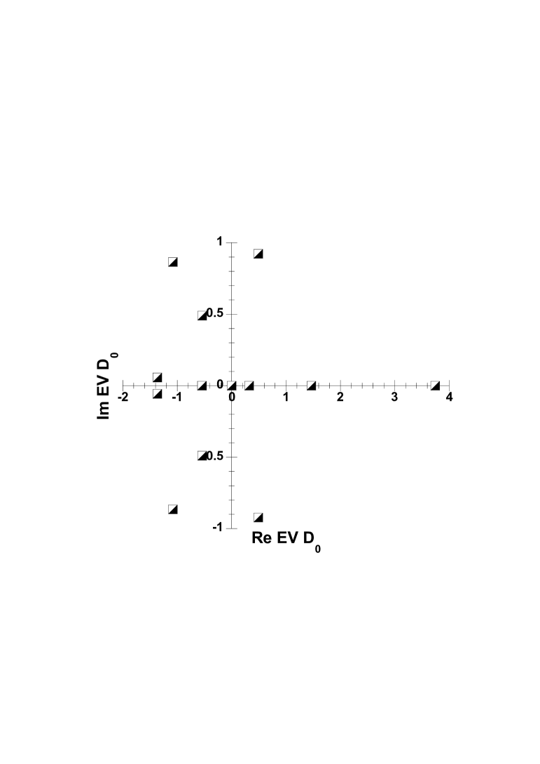
Figure 3: Distribution of the eigenvalues (EVs) of the matrix $D_{0}$ in the complex plane

Figure 4: Distribution of the eigenvalues (EVs) of the matrix $F_{0}$ in the complex plane

Figure 5: Networks of triplets, according to Pajek Manual notations, corresponding to different types of cubic equations as given in the main text; only one network is shown per type of equation; the others can be obtained by permutation.

$M_{0}$	.	.	$M_{0}$	.	.
$EV\;rank$	$Re$	$Im$	$EV\;rank$	$Re$	$Im$
$1$	$7.1039$	-	$62$	$-0.0000$	$-0.0000$
$2$	$1.4849$	$-$	$63$	$-0.3350$	$-$
$3$	$1.0758$	$0.7077$	$64$	$-0.3461$	$0.6531$
$4$	$1.0758$	$-0.7077$	$65$	$-0.3461$	$-0.6531$
$5$	$0.7763$	$-$	$66$	$-0.4422$	$-$
$6$	$0.5693$	$1.3660$	$67$	$-0.4524$	$1.1900$
$7$	$0.5693$	$-1.3660$	$68$	$-0.4524$	$-1.1900$
$8$	$0.4919$	$0.5775$	$69$	$-0.6560$	$-$
$9$	$0.4919$	$-0.5775$	$70$	$-0.7323$	$0.6917$
$10$	$0.3214$	$0.3474$	$71$	$-0.7323$	$-0.6917$
$11$	$0.3214$	$-0.3474$	$72$	$-1.5661$	$0.5212$
$12$	$0.1506$	$0.5245$	$73$	$-1.5661$	$-0.5212$
$13$	$0.1506$	$-0.5245$	$74$	$-1.5739$	$1.2422$
$14$	$0.0000$	$0.0000$	$75$	$-1.5739$	$-1.2422$
$...$	$0.0000$	$0.0000$	$76$	$-1.9041$	$0.1983$
$61$	$-0.0000$	$-0.0000$	$77$	$-1.9041$	$-0.1983$

Table 1: Real ($Re$) and Imaginary ($Im$) part of each eigenvalue (EV) of the $M_{0}$ matrix ranked in increasing rank order according to the $Re$ part. Not all EVs $\equiv 0$ are given.

$C_{0}$	.	.	$D_{0}$	.	.
$EV\;rank$	$Re$	$Im$	$EV\;rank$	$Re$	$Im$
$1$	$3.054$	$-$	$1$	$3.744$	$-$
$2$	$0.4714$	$0.9238$	$2$	$1.4677$	-
$3$	$0.4714$	$-0.9238$	$3$	$0.4907$	0.9230
$4$	$0.3349$	$-$	$4$	$0.4907$	-0.9230
$5$	$0.0000$	$0.0000$	$5$	$0.3213$	-
$6$	$0.0000$	$0.0000$	$6$	$0.0000$	0.0000
$...$	$0.0000$	$0.0000$	$...$	$0.0000$	$0.0000$
$32$	$0.0000$	$0.0000$	$32$	$0.0000$	$0.0000$
$33$	$-0.4441$	$0.7369$	$33$	$0.0000$	0.0000
$34$	$-0.4441$	$-0.7369$	$34$	$-0.5423$	0.4902
$35$	$-0.7072$	$-$	$35$	$-0.5423$	-0.4902
$36$	$-1.0000$	$-$	$36$	$-0.5441$	-
$37$	$-1.7363$	$-$	$37$	$-1.0789$	0.8657
			$38$	$-1.0789$	-0.8657
			$39$	$-1.3640$	0.0572
			$40$	$-1.3640$	-0.0572

Table 2: Real ($Re$) and Imaginary ($Im$) part of each eigenvalue (EV) of the $C_{0}$ and $D_{0}$ matrix ranked in increasing rank order according to the $Re$ part. Not all EVs $\equiv 0$ are given.

$F_{0}$	.	.	$F_{0}$	.	.
$EV\;rank$	$Re$	$Im$	$EV\;rank$	$Re$	$Im$
$1$	$3.8191$	-	$73$	$-$	$0.7097$
$2$	$0.7411$	$0.2997$	$74$	$-$	$-0.7097$
$3$	$0.7411$	$-0.2997$	$75$	$-0.7411$	$0.2997$
$4$	$0.000$	$0.000$	$76$	$-0.7411$	$-0.2997$
$...$	$0.000$	$0.000$	$77$	$-3.8191$	$-$

Table 3: Real ($Re$) and Imaginary ($Im$) part of each eigenvalue (EV) of the $F_{0}$ matrix ranked in increasing rank order according to the $Re$ part. Not all EVs $\equiv 0$ are given

$number$ $of$		$M_{0}$	$C_{0}$	$D_{0}$	$F_{0}$
$nodes$ ($l_{M}$)		$77$	$37$	40	$77$
$links$		$281$	$91$	71	$119$
$directed$ $links$		$219$	$79$	51	$89$
$undirected$ $links$		$31$	$6$	10	$15$
$finite$ $EVs$		$28$	$9$	12	$8$
$EV\equiv 1$		$0$	$0$	0	$0$
$EV\equiv 0$		$49$	$28$	28	$69$
$EV\equiv-1$		$0$	$0$	1	$0$
$real,deg.$ $EV\neq 0$		0	0	0	0
$\rho$ $Re>0$		$3$	$2$	3	$1$
$\nu$ $Re<0$		$3$	$3$	1	$1$
$\mu$ $Im>0$		$0$	$0$	0	$1$
$\mu$ $Im<0$		$0$	$0$	0	1
$\lambda$, $c.c.$ $EV$		11x2	2x2	4x2	3x2
($\lambda_{1}$/$l_{M}$) ln[$\lambda_{1}$/$l_{M}$]		$-0.2199$	$-0.2059$	-0.2217	$-0.1490$
$H_{1}$		$0.7801$	$0.7941$	0.7783	$0.8510$
$H^{{}^{\prime}}_{TC}$		$+0.2655$	+1.0731	$+0.3366$	$+0.8671$
$H^{{}^{\prime\prime}}_{TC}$		$-0.4568$	$-0.2877$	$-0.4346$	$-0.2132$
$H^{{}^{\prime}}_{PV}$		$-0.3889$	+0.7911	$-0.03040$	+0.7603
$H^{{}^{\prime\prime}}_{PV}$		$-0.1328$	$-0.2924$	$-0.04273$	$-0.2422$

Table 4: Pertinent characteristics of studied matrices

References

- [1] I. Procaccia, Nature 333, 498 (1988)
- [2] I. F. Wilde, Lecture notes on complex analysis (Imperial College Press, London, 2006)
- [3] M. Ausloos, J.B. Sousa, M.M. Amado, R.P. Pinto, Appl. Phys. Lett. 43, 927 (1983)
- [4] M. Ausloos, in Non linear Phenomena at Phase Transitions and Instabilities, ed. T.Riste, Plenum Press, New York (1982) pp. 337-341.
- [5] N. Hatano, D.R. Nelson, Phys. Rev. Lett. 77, 570 (1996)
- [6] R. Grobe, F. Haake, H.-J. Sommers, Phys. Rev. Lett. 61, 1899 (1988)
- [7] Y.V. Fyodorov, B.A. Khoruzhenko, Phys. Rev. Lett. 83, 65 (1999)
- [8] M.A. Stephanov, Phys. Rev. Lett. 76, 4472 (1996)
- [9] P. Di Francesco, M. Gaudin, C. Itzykson, F. Lesage, Int. J. Mod. Phys. A 9, 4257 (1994)
- [10] B. Jancovici, Molec. Phys. 42, 1251 (1984)
- [11] P.J. Forrester, B. Jancovici, Int. J. Mod. Phys. A 11, 941 (1996)
- [12] K. Huang, Statistical Mechanics (Wiley, New York, 1963)
- [13] C. Shannon, Bell. Syst. Tech. J. 27, 379 (1948); , Bell. Syst. Tech. J. 27, 623 (1948); see also , Bell Syst. Tech. J. 30, 50 (1951)
- [14] H.E. Stanley, Phase transitions and critical phenomena (Clarendon Press, London, 1971)
- [15] M.E. Fisher, Rev. Mod. Phys. 70, 653 (1998)
- [16] H. E. Stanley, Rev. Mod. Phys. 71, 358 (1999)
- [17] C.J. Thompson, Mathematical statistical mechanics (Macmillan, London, 1971)
- [18] E. Brezin, J.C. LeGuillou, J. Zinn-Justin, Phys. Rev. Lett. 32, 473 (1974)
- [19] J.C. Anifrani, C. Le Floc’h, D. Sornette, B. Souillard, J. Physique I (France) 5, 631 (1995)
- [20] D. Sornette, Phys. Rep. 297, 239 (1998)
- [21]
- [22] H. Theil, Econometrica 33, 67 (1965)
- [23] J. Miśkiewicz, Physica A 387, 6595 (2008)
- [24] F.O. Redelico, A.N. Proto, Int. J. Bifurcation Chaos 20, 413 (2010)
- [25] Q. Wang, Y. Shen, J.Q. Zhang, Physica D 200, 287 (2005)
- [26] K.W. Boyack, S. Milojević, K. Börner, S. Morris, in A. Scharnhorst, K. Börner, P. van den Besselaar (eds.), Models of Science Dynamics, Understanding Complex Systems, (Springer-Verlag Berlin Heidelberg, 2012) pp. 3-22
- [27] Y. Li, H.D. Cao, Y. Tan, Complexity 17, 13 (2011)
- [28] R. Sinatra, D. Condorelli, V. Latora, Phys. Rev. Lett. 105, 178702 (2010)
- [29] V. Venkatasubramanian, S. Katare, P. R. Patkar, F.-P. Mu, Comput. Chem. Eng. 28, 1789 (2004)
- [30] T. Araújo, R. Vilela Mendes, Complex Systems, 12, 357 (2000)
- [31] L. Kullmann, J. Kertész, K. Kaski, Phys. Rev. E 64, 057105 (2001)
- [32] L. Guo, Xu Cai, Int. J. Mod. Phys. C 19, 1909 (2008)
- [33] S. Abe, N. Suzuki, Europhys. Lett. 65, 581 (2004)
- [34] B. Tadić, Physica A 286, 509 (2001)
- [35] G. Mukherjee, S.S. Manna, Phys. Rev. E 71, 066108 (2005)
- [36] L. A. Meyers, M.E.J. Newman, B. Pourbohloul, J. Theor. Biol. 240, 400 (2006)
- [37] E.A. Leicht, M.E.J. Newman, Phys. Rev. Lett. 100, 118703 (2008)
- [38] A. Ramzanpour, V. Karimipour, Phys. Rev. E 66, 036128 (2002)
- [39] A.D. Sánchez, J.M. López, M.A. Rodríguez, Phys. Rev. Lett. 88, 048701 (2002)
- [40] F. Radicchi, S. Fortunato, A. Vespignani, in A. Scharnhorst, K. Börner, P. van den Besselaar (eds.), Models of Science Dynamics, Understanding Complex Systems (Springer-Verlag Berlin Heidelberg, 2012) pp. 233-257
- [41] M. Szell, R. Lambiotte, S. Thurner, Proc. Natl. Acad. Sci. 107, 13636 (2010).
- [42] A. Garcia Cantù Ross, M. Ausloos, Scientometrics 80, 457 (2009)
- [43] G. Rotundo, M. Ausloos, Physica A 389, 5479 (2010)
- [44] A. Bermann, N. Shaked-Monderer, Nonnegative matrices and digraphs, Encyclopedia of Complexity and System Science (Springer, 2008)
- [45] O. Perron, Math. Ann. 64, 248 (1907)
- [46] G. Frobenius, S.-B. Prüss. Acad. Wiss. Berlin (1912) pp. 456-477.
- [47] R.A. Brualdi,
- [48] R.B. Bapat, T.E.S. Raghavan, Nonnegative Matrices and Applications, Encyclopedia of Mathematics and its Applications 64 (Cambridge University Press, Cambridge, 1997)
- [49] A. Berman, M. Neumann, R.J. Stern, Nonnegative Matrices in Dynamic Systems (Wiley-Interscience, 1989)
- [50] A. Berman, R.J. Plemmons, Nonnegative Matrices in the Mathematical Sciences. Classics in Applied Mathematics (SIAM, Philadelphia, PA, 1994)
- [51] H. Minc, Nonnegative Matrices (Wiley, New York, 1988)
- [52] U. Rothblum, Nonnegative matrices and stochastic matrices, in L. Hogben, editor, Handbook of Linear Algebra (CRC Press, 2006)
- [53] E. Senata, Nonnegative Matrices and Markov Chains, Springer Series in Statistics (Springer-Verlag, 1981)
-
[54]
C. Meyer, Matrix analysis and applied linear algebra, ch. 8.3, p. 670 (2000);
. - [55] F.R. Gantmacher, The Theory of Matrices, K.A. Hirsch, transl. 2000, chapter XIII.3, p. 66 (AMA Chelsea Publ., 2000)
- [56] R.E. Tarjan, SIAM Journal on Computing 1, 146 (1972)
- [57] B. Karrer, M.E.J. Newman, Phys. Rev. E 80, 046110 (2009)
- [58] W. Zweger, J. Phys. A: Math. Gen. 18, 2079 (1985)
- [59] J.S. Langer, Ann. Phys. NY 54, 258 (1969)
- [60] W. Cook, C. Mounfield, P. Ormerod, L. Smith, Eur. Phys. J. B 27, 189 (2002)
- [61] G. Livan, L. Rebecchi, Asymmetric correlation matrices: an analysis of financial data, arXiv:1201.6535v2
- [62] S. Droźdź, J. Kwapień, A. Z. Gorski, P. Oswieçimka, Acta Phys. Pol. B 37, 3039 (2006)
- [63] C. Tsallis, J. Stat. Phys. 52, 479 (1988)
- [64] C. Tsallis, R.S. Mendes, A.R. Plastino, Physica A 261, 534 (1998)
- [65] C. Tsallis, Braz. J. Phys. 29, 1 (1999)
- [66] G. Wilk, Z. Wlodarczyk, Acta Phys. Pol. B 35, ) 871 (2004
- [67] M. Ausloos, J. Miśkiewicz, Braz. J. Physics 39, 388 (2009)
- [68] J.R. Iglesias, R.M.C. de Almeida, Eur. Phys. J. B 85: 85 (2012)
- [69] J. Moody, Social Networks 20, 291 (1998)
- [70] R. Milo, S. Shen-Orr, S. Itzkovitz, N. Kashtan, D. Chklovskii, U. Alon, Science, 298, 824 (2002)
- [71] R. Milo, S. Itzkovitz, N. Kashtan, R. Levitt, S. Shen-Orr, I. Ayzenshtat, M. Sheffer, U. Alon, Science 303, 1538 (2004)
- [72] V. Batagelj, A. Mrvar, Pajek, Program for Analysis and Visualization of Large Networks Reference Manual, Fig. 15, p. 52