Quantum-mechanical engine models and their efficiencies

Abstract

Based on quantum thermodynamic processes, we make a quantum-mechanical (QM) extension of the typical heat engine cycles, such as the Carnot, Brayton, Otto, and Diesel cycles, etc. The temperature is not included in these QM engine cycles, as lies in the fact that the concept of energy is well-defined in quantum mechanics, temperature a priori is not. These QM engine cycles are implemented by an ideal or interacting system with an arbitrary number of particles confined in an arbitrary power-law trap. As a result, a relation between the quantum adiabatic exponent and trap exponent is found. The efficiency of a given QM engine cycle is similar to that of its classical counterpart, thereby identifying the universality of the efficiency.

PACS number(s): 05.70.-a, 03.65. -w, 51.30+i

The current activities in quantum thermodynamics Gem09 focus on quantum heat engines Scu03 ; Quan07 ; Quan09 ; Fia12 ; Kim11 ; Gev92 ; Ben00 ; Abe12 ; pre1104 ; pre12III ; pre1204 ; Lu12 ; Wu06 ; Rez06 ; Fel00 ; pre1203 ; Huang12 ; Per98 or refrigerators Cle12 ; He02 , work-extraction processes Kie04 ; All08 ; Hul12 from quantum systems, and positive work conditions Quan05 . Among all the studies about quantum thermodynamics, a central concern is to make a quantum extension Quan07 ; Quan09 ; Ben00 of classical thermodynamic processes and cycles. As in classical thermodynamics, for quantum thermodynamics there are some basic thermodynamic processes: isothermal, adiabatic, isochoric, isobaric, and isoenergetic processes. These processes correspond to constant temperature, entropy, volume, pressure, and energy, respectively. They can be used to construct all kinds of thermodynamic cycles, such as the Carnot, Brayton, Otto, Diesel, Ericsson, and Stirling cycles, etc. Because of quantum features of the working substance, unusual and exotic behaviors have been found in quantum heat engines. A prominent example is a quantum heat engine which may use an isolated finite system as its working substance to produce work Fia12 . In an isolated finite system Hui11 as well as quantum mechanics, the concept of energy (rather than temperature) is well-defined. Recently, a quantum-mechanical (QM) Carnot cycle working between two energy baths instead of heat baths has been generalized and studied intensively Ben02 ; Abe12 ; pre12III since it was first proposed by Bender et al Ben00 . Nevertheless, little attention was paid to such a QM generalization of the remaining classical thermodynamic processes and cycles until most recently pre1204 .

In this paper, we study various quantum thermodynamic processes and their related quantum thermodynamic cycles. We begin our analysis with the definitions of quantum thermodynamic processes, including isoenergetic, isobaric, and isochoric processes, and with clarification of how to achieve these processes. The generalization of these processes allows us to study an arbitrary quantum thermodynamic cycle constructed by any four of these processes. We discuss various quantum thermodynamic cycles, such as the QM Carnot, Brayton, Otto, and Diesel cycles, etc., and compare their properties with their classical counterparts. From these comparisons, the universality of the efficiency is identified for a given cycle.

Various thermodynamic processes for a QM system. For a QM system, the expectation value of the system Hamiltonian is given by $E=\langle\psi|{H}|\psi\rangle=\sum_{n}p_{n}{\varepsilon_{n}},$ where $\varepsilon_{n}$ is the single-particle energy spectrum and $p_{n}$ is the mean occupation probability of the $n$th eigenstate, with $n=1,2,3,\cdots$. The derivation of $E$ leads to the first law of quantum thermodynamics Quan09 ; Kim11 ; pre1203 : $dE={\mathchar 22\relax\mkern-12.0mud}Q+{\mathchar 22\relax\mkern-12.0mud}W=\sum_{n}\varepsilon_{n}dp_{n}+\sum_{n}p_{n}d\varepsilon_{n}$, where ${\mathchar 22\relax\mkern-12.0mud}Q=\sum_{n}\varepsilon_{n}dp_{n}$ and ${\mathchar 22\relax\mkern-12.0mud}W=\sum_{n}p_{n}d\varepsilon_{n}$ are associated with the energy exchange and work done, respectively. That is, energy exchange between a QM system and its surroundings is induced by transitions between quantum states of the system, in which whether temperature (heat bath) is included or not, while work is performed due to variation of energy spectrum with fixed occupation probabilities. As in a classical system where the generalized force $Y_{n}$, conjugate to the generalized coordinate $y_{n}$, is defined by $Y_{n}=-\frac{{\mathchar 22\relax\mkern-12.0mud}W}{d{y_{n}}}$, the force for a quantum system can be defined as

$$F=-\frac{{\mathchar 22\relax\mkern-12.0mud}W}{dL}=-\sum_{n}{p_{n}}\frac{d\varepsilon_{n}}{dL}.$$ (1)

Here $L$ as the generalized coordinate corresponds to the force $F$, which is, in fact, the pressure of the quantum system.

Without loss of generality, we consider a quantum system which consists of an arbitrary number of ideal or interacting particles confined in an arbitrary power-law trap. A one-dimensional power-law trap can be parameterized by a single-particle energy spectrum of the form epjd ; Wil97 ; pre1104

$$\varepsilon_{n}=\hbar\omega n^{\sigma}=\hbar\lambda L^{-\theta}n^{\sigma},$$ (2)

where $n$ is a positive integer quantum number, and $\sigma$ is an index of the single-particle energy spectrum. Here we have used the relation $\omega=\lambda L^{-\theta}$, where $\lambda$ is a constant for a given potential, and $\theta$ is trap exponent wpra09 depending on the trapping potential pre1104 . Note that the energy spectrum (2) can also be used to depict the other physical systems, such as a harmonic system Gev92 , a spin-$1/2$ system Huang12 ; Gev92 , and a single-mode radiation field in a cavity pre1104 , etc. It follows, on substitution of Eq. (2) into Eq. (1), that the force acting on the potential wall is

$$F=\theta\sum_{n}p_{n}\frac{\varepsilon_{n}}{L},$$ (3)

from which, the internal energy $E_{i}$ of the system at any instant $i$ can be derived as

$$E_{i}=\sum_{n}p_{n}\varepsilon_{n}=L_{i}F_{i}/\theta.$$ (4)

To realize an isoenergetic process pre12III , the system exchanges energy with an energy bath so that the work done by the external parameter $\lambda$, on which the Hamiltonian of the quantum system depends parametrically, can be precisely counterbalanced. In the isoenergetic process, the quantum system evolves from an initial state $|\psi(0)\rangle$ to a final state $|\psi(t)\rangle$ through a unitary evolution. One possible way of achieving this is to demand the constancy of the expectation of the Hamiltonian in such a way that $\frac{d{H}}{dt}=[{H}(t),{H}(t^{\prime})]+\frac{\partial{H}}{\partial t}=[{H}(t),{H}(t^{\prime})]+\frac{\partial{H}}{\partial\lambda}\frac{\partial\lambda}{\partial t}=0$, where $0\leq t<t^{\prime}\leq t_{ie}$ with $t_{ie}$ being the time required for completing the isoenergetic process.

Both the system volume $L$ and the occupation probabilities $p_{n}$ change in the isoenergetic process, and the system exchanges energy with the energy bath in order for the system energy $E(L)$ to be kept constant. So the energy exchange is a form of heat exchange by definition, and the external energy baths play the role of heat baths in conventional heat engines. According to the first law of thermodynamics, energy absorbed by the system in an isoenergetic process, with constant energy $E_{if}$, can be determined according to

$$Q_{if}=\int_{L_{i}}^{L_{f}}F_{if}dL=\theta E_{if}\ln{(L_{f}/L_{i})},$$ (5)

where we have used $Q_{if}=W_{if}$ in the isoenergetic process.

For a quantum isobaric process with constant pressure, the time scale of relaxation of the system with the heat bath should be much smaller than that of the variation of the system volume Lin76 ; Quan09 . If a classical or a quantum system coupled to a heat bath undergoes an isobaric process, we must carefully control the temperature of the system as well as the temperature of the heat bath under some conditions that sensitively depend on the systems Quan09 , when we change the volume of the system. This is not the case in the absence of a heat bath. In contrast, we can see from Eq. (3) that $LF(L)/E=\texttt{cons},$ which can be regarded as the equation of state for the system under consideration. The energy of the system undergoing a quantum isobaric process only needs to be controlled in such a way that $E\propto L$, which is independent of the form of the trapping potential. Similar to a quantum isoenergetic process, the controlled parameter in a quantum isobaric process is switched from $\lambda(0)$ to $\lambda(t_{ib})$ in a period $t_{{ib}}$. One possible way to achieve the constant-pressure process is that the pressure $F(\lambda)$, other than the Hamiltonian $H$, should satisfy the condition: $\frac{d{F}}{dt}=[{F}(t),{H}(t^{\prime})]+\frac{\partial{F}}{\partial t}=[{F}(t),{H}(t^{\prime})]+\frac{\partial{F}}{\partial\lambda}\frac{\partial\lambda}{\partial t}=0,$ where $0\leq t<t^{\prime}\leq t_{ib}$.

For an isobaric expansion $i\rightarrow f$, the energy transferred to the system not only produces work $W_{if}=(L_{f}-L_{i})F_{if}$ but also changes the energy of the system $\Delta E=E_{f}-E_{i}$. The energy absorbed by the system in the isobaric expansion, $Q_{if}$, is therefore obtained by use of Eq. (4),

$$Q_{if}=E_{f}-E_{i}+W_{if}=\frac{\theta+1}{\theta}{(L_{f}-L_{i})}F_{if}.$$ (6)

An isochoric process is one in which the volume $L$ is held constant, meaning that, while no work is done by the system, energy as a form of heat is exchanged between the working substance and the energy bath. The transitions between quantum states as well as the variation of occupation probabilities in an atomic system are achieved when the system interacts with an external field pre1204 , which can be regarded as a good example of a quantum isobaric process without introduction of temperature. The condition that the working substance should reach thermal equilibrium with the heat bath at the end of a conventional quantum as well as classical isochoric process Quan07 is therefore no longer required to be fulfilled in such a quantum isochoric process. Energy quantity absorbed by the system during a quantum isochoric process $i\rightarrow f$ is given by

$$Q_{if}=E_{f}-E_{i}.$$ (7)

Although the conditions that realize the quantum isobaric and isochoric processes without inclusion of temperature are different from corresponding ones with introduction of temperature, the heat exchanges between the system and its surroundings are easily proved to be still given by Eqs. (6) and (7) in the presence of a heat bath.

The quantum adiabatic process has been extensively clarified in many references Quan09 ; Foc28 ; pre12III ; arx12 ever since the birth of quantum mechanics. A quantum adiabatic process must proceed at a very slow speed so that the time scale of the change of the system state must be larger than that of the dynamical one, $\sim\hbar/E$ Foc28 ; Abe12 ; pre12III and thus the generic quantum adiabatic condition Foc28 is satisfied. The occupation probabilities remain unchanged, $dp_{n}=0$, which, together with the relation ${\mathchar 22\relax\mkern-12.0mud}Q=\sum_{n}\varepsilon_{n}dp_{n}$, means that there is no heat exchange in a quantum adiabatic process.

Given a trapping potential, the index $\sigma$ of the energy spectrum and the trap exponent $\theta$ are fixed. Thus, for a quantum system undergoing an adiabatic process, we have

$$L^{\theta+1}F=\texttt{cons}.$$ (8)

Through comparison with $L^{\gamma}F=\texttt{cons}$ for the classical adiabatic process, the adiabatic exponent is obtained,

$$\gamma=\theta+1,$$ (9)

which bridges the trap exponent $\theta$ and the adiabatic exponent $\gamma$. As an example, the trap exponent $\theta=2$ for a one-dimensional box trap, and thus the adiabatic exponent $\gamma=3$ in this case, confirming the result obtained previously in a different way Quan09 . The relation between the trap and adiabatic exponents given by Eq. (9) can also be derived very easily even if temperature is included note3 .

Various QM Engines And Their Efficiencies. It is well known that any device, such as a heat engine, or a fuel cell, is described by its efficiency: the relationship between the total energy input, and the amount of energy used to produce useful work. To describe the performance of a QM engine, we follow this definition of the efficiency: the amount of energy input that is actually converted to useful output. A QM Carnot cycle is a QM analog of the classical as well as conventional quantum Carnot cycle, which consists of two quantum isoenergetic processes and two quantum adiabatic processes, as shown in Fig. 1(a). The efficiency of the quantum Carnot cycle is given by

$$\eta_{C}=1-\frac{Q_{34}}{Q_{12}}=1-\frac{E_{34}\ln{(L_{3}/L_{4})}}{E_{12}\ln{(L_{2}/L_{1})}},$$ (10)

where we have used Eq. (5). Defining $E_{h}=E_{12}$, and $E_{c}=E_{34}$, using Eq. (4), the two constant energies of the system $E_{h}$ and $E_{c}$ can be expressed as $E_{h}=F_{1}L_{1}/\theta=F_{2}L_{2}/\theta$ and $E_{c}=F_{3}L_{3}/\theta=F_{4}L_{4}/\theta$. These two equations together with $L_{2}^{\theta+1}F_{2}=L_{3}^{\theta+1}F_{3}$ and $L_{1}^{\theta+1}F_{1}=L_{4}^{\theta+1}F_{4}$ obtained from Eq. (8), give rise to the relation $L_{2}/L_{1}=L_{3}/L_{4}$. Hence, the efficiency of the QM Carnot engine becomes

$$\eta_{C}=1-\frac{E_{c}}{E_{h}}.$$ (11)

This result obtained earlier Ben00 ; Abe12 ; pre12III , is the same as that of a classical as well as quantum Carnot cycle working between two heat reservoirs, with the identification of the system energy as the temperature of the system, but it is derived here in a general way.

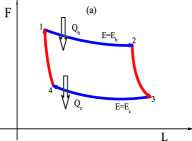
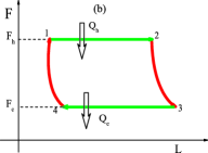
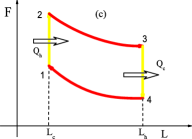
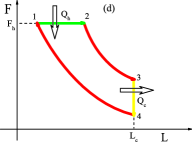
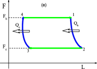
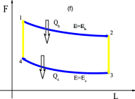
Figure 1: (Color online) Graphic diagrams of QM (a) Carnot, (b) Brayton, (c) Otto, (d) Diesel, (e) Ericsson, and (f) Stirling cycles, in the plane of $(L,F)$. The isoenergetic, adiabatic, isobaric, and isochoric processes, are indicated by the blue, red, green, and yellow lines.

A QM Brayton cycle, consisting of two quantum isobaric and two quantum adiabatic processes, is illustrated in Fig 1(b). Using Eq. (6) and the fact that no heat exchange occurs in two adiabatic processes, it follows that the efficiency of a quantum Brayton cycle is

$$\eta_{B}=1-\frac{Q_{34}}{Q_{12}}=1-\frac{(L_{3}-L_{4})F_{34}}{(L_{2}-L_{1})F_{12}}.$$ (12)

For two adiabatic processes $2\rightarrow 3$ and $4\rightarrow 1$, from Eq. (8) we have $L_{2}^{\theta+1}F_{12}=L_{3}^{\theta+1}F_{34}$ and $L_{1}^{\theta+1}F_{12}=L_{4}^{\theta+1}F_{34}$. Subtracting both sides of these two equations, we can find,

$$\frac{L_{2}-L_{1}}{L_{3}-L_{4}}={\left(\frac{F_{34}}{F_{12}}\right)}^{\frac{1}{\theta+1}}.$$ (13)

Substitution of Eq. (13) into Eq. (12) leads to

$$\eta_{B}=1-\left(\frac{F_{34}}{F_{12}}\right)^{1-1/\gamma}.$$ (14)

In deriving Eq. (14), the relation between $\theta$ and $\gamma$ given by Eq. (9) has been used. This efficiency of the QM Brayton engine is identical to that of a classical Brayton cycle Per98 .

The engines operating by Otto cycle have been widely used in automobiles as well as the internal combustion engines Quan07 . A QM Otto cycle consisting of two isochoric and two adiabatic processes is illustrated in Fig. 1(c). The efficiency of the quantum Otto cycle can be expressed in terms of pressures and potential widths at special instants,

$$\eta_{O}=1-\frac{L_{3}F_{3}-L_{4}F_{4}}{L_{2}F_{2}-L_{1}F_{1}}.$$ (15)

where $F_{i}$ and $L_{i}$, with $i=1,2,3,4$, are pressures and potential widths at four instants $1,2,3,$ and $4$. By denoting $L_{c}=L_{1}=L_{2}$ and $L_{h}=L_{3}=L_{4}$ and using Eq. (8), we further simplifies Eq. (15) to

$$\eta_{O}=1-\left(\frac{L_{c}}{L_{h}}\right)^{\theta}=1-\left(\frac{L_{c}}{L_{h}}\right)^{\gamma-1},$$ (16)

which is the same as the efficiency of the classical Otto engine.

Besides two quantum adiabatic processes $2\rightarrow 3$ and $4\rightarrow 1$, the Diesel cycle consists of an isobaric process $1\rightarrow 2$ and an isochoric process $3\rightarrow 4$ [see Fig. 1(d)]. The efficiency of the quantum Diesel cycle can be expressed in terms of pressures and potential widths at special instants,

$$\eta_{D}=1-\frac{\theta(E_{3}-E_{4})}{(\theta+1)(L_{2}-L_{1})F_{h}},$$ (17)

where we have taken $F_{h}=F_{1}=F_{2}$. Using $F_{h}L_{1}^{\theta+1}=F_{4}L_{3}^{\theta+1}$ and $F_{h}L_{2}^{\theta+1}=F_{3}L_{3}^{\theta+1}$, and $E_{i}=F_{i}L_{i}/\theta$, with $i=3,4$, we obtain $\eta_{D}=1-\frac{1}{\theta+1}\frac{L_{2}^{\theta+1}-L_{1}^{\theta+1}}{(L_{2}-L_{1})L_{3}^{\theta}},$ or

$$\eta_{D}=1-\frac{1}{\gamma}\frac{\left(\frac{L_{2}}{L_{c}}\right)^{\gamma}-\left(\frac{L_{1}}{L_{c}}\right)^{\gamma}}{\left(\frac{L_{2}}{L_{c}}\right)-\left(\frac{L_{1}}{L_{c}}\right)},$$ (18)

which is identical to its classical counterpart. In deriving Eq. (18) we have used Eq. (9) and $L_{c}\equiv L_{3}$.

A QM Ericsson (Stirling) cycle consists of two quantum isoenergetic and two quantum isobaric (isochoric) processes. The schematic diagram of the QM Ericsson as well as Stirling cycle is plotted in Fig. 1. From Eq. (4), we find, in two isobaric processes of the Ericsson cycle [see Fig. 1(e)], $L_{1}F_{41}=L_{2}F_{23}$ and $L_{3}F_{23}=L_{4}F_{41}$, where use of $F_{1}=F_{4}=F_{41}$ and $F_{2}=F_{3}=F_{23}$ has been made. Hence, the amount of energy transported from the system, $Q_{23}=(L_{3}-L_{2})F_{23}$, is equal to that of energy absorbed by the system, $Q_{41}=(L_{4}-L_{1})F_{41}$. The efficiency of the QM Ericsson engine is still given by the QM version of the Carnot efficiency, $\eta_{E}=\eta_{C}=1-E_{c}/E_{h}$. In view of the fact that no work is done in an isochoric process, we find that the energy absorbed by the system during the isochoric process $2\rightarrow 3$, $Q_{23}=E_{h}-E_{c}$, is totally counterbalanced by the energy released to the system in the isochoric process $4\rightarrow 1$, $Q_{41}=E_{h}-E_{c}$ [see Fig. 1(f)]. The expression of efficiency for the QM Stirling engine is thus the same as that for the QM Carnot as well as Ericsson engine, namely, $\eta_{S}=1-{E_{c}}/{E_{h}}$.

Before ending this section, we would like to emphasize that the energy spectrum as well as the occupation probabilities considered here are general and intrinsic. Therefore, our result in the present paper is independent of any parameter contained in the system, whether the interaction between particles is considered or not, and it is indeed valid for an arbitrary ideal or interacting system, such as a system with an arbitrary number of particles in an arbitrary power-law trap, a harmonic system, a spin-$1/2$ system, and a single-mode radiation field, and so on.

Conclusion. We have studied the energy analogy of the classical thermodynamic cycles based on microscopic definitions of various thermodynamic processes. We have clarified the properties of these quantum thermodynamic processes and cycles, bridging the quantum thermodynamic cycles and their classical counterparts. Comparison between quantum adiabatic process and its classical counterpart gives rise to a relation between the trap exponent and the quantum adiabatic exponent. The universality of the efficiency for any given cycle is identified, in the sense that the expression of the efficiency is intrinsic and independent of any parameter involved in a given engine model.

Acknowledgements: We gratefully acknowledge support for this work by the National Natural Science Foundation of China under Grants No. 11265010, No. 11147200, No. 11065008, No. 10974033, and No. 11191240252, the State Key Programs of China under Grant No. 2012CB921604, and the Foundation of Jiangxi Educational Committee under Grant No. GJJ12136. J. H. Wang is very grateful to Haitao Quan for his valuable discussions.

References

- (1) J. Gemmer, M. Michel, and G. Mahler, Quantum Thermodynamics, 2nd ed. (Springer-Verlag, Berlin, 2009).
- (2) P. Perrot, A to Z of Thermodynamics (Oxford University Press, Oxford, 1998).
- (3) E. Geva and R. Kosloff, J. Chem. Phys. 96, 3054 (1992); J. Chem. Phys. 97, 4396(1992); J. Chem. Phys. 102, 8541 (1995); R. Kosloff, E. Geva, and J. Gordon, J. Appl. Phys. 87, 8093 (2000).
- (4) M. O. Scully, M. S. Zubairy, G. S. Agarwal, and H. Walther, Science 299, 862 (2003).
- (5) S. W. Kim, T. Sagawa, S. De Liberato, and M. Ueda, Phys. Rev. Lett. 106, 070401 (2011).
- (6) O. Fialko and D. W. Hallwood, Phys. Rev. Lett. 108, 085303 (2012).
- (7) H. T. Quan, Y. X. Liu, C. P. Sun, and F. Nori, Phys. Rev. E 76, 031105 (2007).
- (8) H. T. Quan, Phys. Rev. E 79, 041129 (2009).
- (9) C. M. Bender, D. C. Brody, and B. K. Meister, J. Phys. A: Math. Gen. 33, 4427 (2000).
- (10) S. Abe, Phys. Rev. E 83, 041117 (2011); S. Abe and S. Okuyama, Phys. Rev. E 83, 021121 (2011); S. Abe and S. Okuyama, Phys. Rev. E 85, 011104 (2012).
- (11) J. H. Wang, J. Z. He, and Z. Q. Wu, Phys. Rev. E 85, 031145 (2012).
- (12) J. H. Wang, J. Z. He, and X. He, Phys. Rev. E 84, 041127 (2011).
- (13) R. Wang, J. H. Wang, J. Z. He, and Y. L. Ma, Phys. Rev. E 86, 021133 (2012); J. H. Wang and J. Z. He, J. Appl. Phys. 11, 043505 (2012).
- (14) J. H. Wang, Z. Q. Wu, and J. Z. He, Phys. Rev. E 85, 041148 (2012).
- (15) Y. Lu and G. L. Long, Phys. Rev. E 85, 011125 (2012).
- (16) T. Feldmann and R. Kosloff, Phys. Rev. E 61, 4774 (2000); T. Feldmann and R. Kosloff, Phys. Rev. E 68, 016101 (2003); T. Feldmann and R. Kosloff, Phys. Rev. E 70, 046110 (2004).
- (17) F. Wu, L. G. Chen, S. Wu, F. R. Sun, and C. Wu, J. Chem. Phys. 124, 214702 (2006); F. Wu, L. G. Chen, F. R. Sun, C. Wu, and Q. Li, Phys. Rev. E 73, 016103 (2006).
- (18) Y. Rezek and R. Kosloff, New J. Phys. 8, 83 (2006).
- (19) X. L. Huang, L. C. Wang, and X. X. Yi, arXiv:1209.1684 [quant-ph].
- (20) J. Z. He, J. C. Chen, and B. Hua, Phys. Rev. E 65, 036145 (2002).
- (21) B. Cleuren, B. Rutten, and C. Van den Broeck, Phys. Rev. Lett. 108, 120603 (2012).
- (22) T. D. Kieu, Phys. Rev. Lett., 93, 140403 (2004).
- (23) A. E. Allahverdyan, R. S. Mahler, and G. Johal, Phys. Rev. E, 77, 041118(2008).
- (24) X. L. Huang, T. Wang, and X. X. Yi, Phys. Rev. E 86, 051105 (2012).
- (25) H. T. Quan, P. Zhang, and C. P. Sun, Phys. Rev. E 72, 056110 (2005).
- (26) J. H. Wang, J. Z. He, and Y. L. Ma, Phys. Rev. E 83, 051132 (2011); H. Y. Tang and Y. L. Ma, Phys. Rev. E 83, 061135 (2011).
- (27) C. M. Bender, D. C. Brody, and B. K. Meister, Proc. R. Soc. Lond. A 458, 1519 (2002).
- (28) J. H. Wang and J. Z. He, Eur. Phys. J. D 64, 73 (2011); J. Low. Temp. Phys. 166, 80 (2012).
- (29) M. Wilkens and C. Weiss, J. Mod. Opt. 44, 1801 (1997); C. Weiss and M. Wilkens, Opt. Express 1, 272 (1997).
- (30) J. H. Wang, H. Y. Tang, and Y. L. Ma, Ann. Phys. 326, 634 (2011), and references therein.
- (31) G. Lindblad, Commun. Math. Phys. 48, 119 (1976); U. Weiss, Quantum Dissipative Systems, 2nd ed. (World Scientific, Singapore, 1999).
- (32) M. Born and V. Fock, Z. Phys. 51, 165 (1928).
- (33) J. H. Wang and J. Z. He, Phys. Rev. E 86, 051112 (2012).
- (34) In the presence of a heat bath, the relation between the trap and adiabatic exponents can be readily obtained without requiring derivation of an explicit function of the entropy . When a -particle quantum system is in thermal equilibrium with a heat reservoir at constant temperature , the occupation probability at any state of the system must satisfy the Boltzmann distribution: , where is the Boltzmann constant and is the canonical partition function. For the quantum adiabatic process the probabilities remain constant thus leading to constant entropy since is determined by . Whereas the temperature varies in an adiabatic process, the ratio should keep fixed in order for which is only the function of to be a constant. Adopting the energy spectrum given by Eq. (2), we find that , which yields the relation through comparison with for the adiabatic process.
- (35) For the convetional Carnot cycle, we find that the Carnot efficiency, , and that . Since the heat exchange in an isobaric (isochoric) process, in which the system couples to a heat bath instead of an energy bath, is still given by Eq. (6)[Eq. (7)], the expressions of the effiencies for the ideal Brayton, Otto, and Diesel cycles are still given by Eqs. (14), (16), and (18), respecively.
- (36) V. Blickle and C. Bechinger, Nat. Phys. 8, 143 (2012).