Einstein@Home Discovery of 24 Pulsars in the Parkes Multi-beam Pulsar Survey

Abstract

We have conducted a new search for radio pulsars in compact binary systems in the Parkes multi-beam pulsar survey (PMPS) data, employing novel methods to remove the Doppler modulation from binary motion. This has yielded unparalleled sensitivity to pulsars in compact binaries. The required computation time of $\approx 17\,000$ CPU core years was provided by the distributed volunteer computing project Einstein@Home, which has a sustained computing power of about 1 PFlop s${}^{-1}.$ We discovered 24 new pulsars in our search, of which 18 were isolated pulsars, and six were members of binary systems. Despite the wide filterbank channels and relatively slow sampling time of the PMPS data, we found pulsars with very large ratios of dispersion measure (DM) to spin period. Among those is PSR J1748$-$3009, the millisecond pulsar with the highest known DM ($\approx$420 pc cm^-3). We also discovered PSR J1840$-$0643, which is in a binary system with an orbital period of 937 days, the fourth largest known. The new pulsar J1750$-$2536 likely belongs to the rare class of intermediate-mass binary pulsars. Three of the isolated pulsars show long-term nulling or intermittency in their emission, further increasing this growing family. Our discoveries demonstrate the value of distributed volunteer computing for data-driven astronomy and the importance of applying new analysis methods to extensively searched data.

1. Introduction

Einstein@Home is a distributed volunteer computing project: members of the public donate otherwise unused computing cycles on their home and/or office PCs to the project to enable blind searches for unknown neutron stars. The detection of continuous gravitational waves from such sources in data from ground-based interferometric detectors is the main, long-term goal of Einstein@Home (Abbott et al., 2009a, b; Aasi et al., 2012). Recently, successful searches for neutron stars through their radio emission have also been conducted with Einstein@Home (Knispel et al., 2010, 2011; Allen et al., 2013). Here we present the first results from a novel search for radio pulsars in compact binary systems in data from the Parkes multi-beam pulsar survey (PMPS; Manchester et al., 2001).

The discovery and timing of compact binary pulsars is one of the key science drivers for the construction of the Square Kilometre Array (Kramer et al., 2004; Cordes et al., 2004). Such systems provide the most precise ‘laboratories’ for tests of general relativity and alternative theories of gravity in the strong field regime (Taylor & Weisberg, 1989; Kramer et al., 2006b; Freire et al., 2012a, b; Shao & Wex, 2012). The discovery of such systems also has important implications for estimates of the Galactic binary merger rate and for predictions of the expected detection rate of these events in gravitational-wave searches, e.g. (Kim et al., 2003). Furthermore, the study of compact binary pulsars offers unique opportunities to deepen our understanding of the stellar evolution processes forming these systems (Stairs, 2004; Belczynski et al., 2008) and their progenitor stars. Finally, the discovery of pulsars hitherto missed in the PMPS data helps to complete our picture of the Galactic pulsar population and is useful for simulations for which the PMPS is used as a ‘reference survey’ (Lorimer, 2012).

The detection of binary pulsars with standard Fourier methods is hampered by Doppler smearing of the pulsed signal caused by binary motion during the survey observation (Johnston & Kulkarni, 1991). Previous searches for these systems in the PMPS have utilized ‘acceleration searches’ to correct for the line-of-sight motion of the pulsars (Faulkner et al., 2004; Eatough et al., 2013; Eatough, 2009). Although computationally efficient, acceleration techniques are only effective when the observation time is a small fraction of the orbital period and where the acceleration is therefore roughly constant over the duration of the observation. Thus, these techniques are not sensitive to the most compact systems (Ransom et al., 2002).

In this work, the PMPS data have been searched using a method to fully demodulate the pulsar signals in compact binary systems based on a large number of circular orbital templates. The method, which is only possible with the computing resources provided by Einstein@Home, offers un-paralleled sensitivity to systems that would have previously been missed by acceleration searches. Using tailored post-processing methods to identify promising new pulsar candidates generated from the search, we have discovered 24 new pulsars.

A full and detailed description of the Einstein@Home radio pulsar search pipeline can be found in Allen et al. (2013). The goal of this paper is to provide a summary of the Einstein@Home PMPS search and to present our first discoveries. A sensitivity comparison to all previous PMPS analyses, an estimate of the search sensitivity to compact binaries, and implications for the Galactic population of these objects will be discussed in a future paper.

The structure of the rest of this paper is as follows: in Sec. 2 we summarize the main system parameters of the PMPS and previous analyses of the survey data. Sec. 3 explains our new search pipeline in detail, including post-processing methods. In Sec. 4 we present the 24 newly discovered pulsars along with coherent timing solutions in cases where they have been obtained. In Sec. 5 we briefly discuss implications of the search, before concluding. The reader can find technical details of the post-processing in the Appendix.

2. Parkes Multi-Beam Pulsar Survey and Previous Analyses

The PMPS is the most successful pulsar survey ever performed with a yield of over 800 pulsars. The success of the PMPS at discovering pulsars is in part due to the multiple re-analyses of the data using new and improved search methods. In searches for relativistic binary pulsars, this has typically been enabled by an increase in the available computing power, as in the case of this work. Here we outline the survey setup, and previous and on-going analyses of the PMPS data.

PMPS observations were done with the 64-meter Parkes radio telescope and targeted the Galactic plane between $260^{\circ}$ and $50^{\circ}$ Galactic longitude $\ell$ and Galactic latitude $\left|b\right|\leq 5^{\circ}$ with a total of 3190 telescope pointings (Manchester et al., 2001). Each pointing is comprised of 13 dual-polarization beams. These are arranged in two hexagonal rings, each containing six beams around a central beam, creating a ‘Star-of-David’ pattern (Staveley-Smith et al., 1996). Each observation covers a radio bandwidth of 288 MHz, which is observed in a filterbank of 96 channels each with 3 MHz width, centered on 1374 MHz. The sampling time is 250 $\mu$s and the filterbank data have a dynamic range of 1 bit per sample. Each beam has an integration time of 2097.152 s, with $2^{23}$ time samples. This yields a file size of $\approx$100.7 MB per beam and a total data volume of 4.1 TB for all filterbank and associated header files.

The majority of pulsars discovered in the PMPS ($\sim 600$) were found in the original processing of the survey data (Manchester et al., 2001; Morris et al., 2002; Kramer et al., 2003; Hobbs et al., 2004). After these analyses were completed, it was noticed that in comparison to the number of typical isolated pulsars, the number of binary and millisecond pulsars (MSPs) discovered was disproportionally low (Faulkner et al., 2004). For this reason a full re-processing of the survey was performed with acceleration searches, improved radio frequency interference (RFI) filters, and better pulsar candidate selection tools (Faulkner et al., 2004). This analysis resulted in the discovery of a further 124 pulsars, including 15 pulsars with spin periods $<30$ ms. The double neutron star system, PSR J1756$-$2251, was also found and would not have been discovered without acceleration searches (Faulkner et al., 2005). In addition, the results generated by the Faulkner et al. (2004) processing were re-analyzed using new tools for ranking of pulsar candidates, allowing the discovery of another 29 pulsars (Keith et al., 2009).

Searches for binary radio pulsars can be characterized by the ratio of phase-coherently analyzed observation time $T$ to orbital period $P_{\text{orb}}$ of the pulsar. For orbital periods long compared to the observation time, i.e. $T/P_{\text{orb}}\lesssim 0.1$, the signal can be well described assuming a constant acceleration and ‘classical’ acceleration searches are a computationally efficient analysis method (Ransom et al., 2002) with only small sensitivity losses. If multiple orbits fit into a single observation, i.e., $T/P_{\text{orb}}\gtrsim 5$, side-band searches provide a computational short-cut at the cost of a slight loss in sensitivity (Jouteux et al., 2002; Ransom et al., 2003).

The acceleration search technique used by Faulkner et al. (2004) (stack-slide search) was imperfect in two respects. First, the incoherent addition of spectra results in a reduction in sensitivity (see, e.g., Wood et al., 1991 and Brady & Creighton, 2000), and second, the orbital periods to which the method was sensitive were limited $P_{\text{orb}}\gtrsim 10T\gtrsim 6$ hr. These deficiencies were partially addressed by Eatough et al. (2013), where independent halves of the 35 min observation were analyzed with coherent acceleration searches, resulting in a minimum detectable orbital period of $\sim 3$ hr. This search, which also used improved RFI removal techniques and automated pulsar candidate selection tools, resulted in the discovery of 16 pulsars, but no previously un-discovered relativistic binaries.

Recently, Mickaliger et al. (2012) announced the discovery of five MSPs in a re-analysis of the PMPS data. Because no acceleration searches were used in this analysis, the reason these pulsars were missed by previous searches is not yet fully understood.

The improved binary search analysis presented in this work was initiated for two main reasons. Acceleration searches can only probe a limited orbital parameter space. The data segmentation approach by Eatough et al. (2013) is sensitive to a larger orbital parameter space but loses sensitivity due to shorter coherent observation times. As we will show below our search further expands the orbital parameter search while using the full coherent observation time.

3. The Einstein@Home Analysis of the PMPS Data

The intermediate range $0.1\lesssim T/P_{\text{orb}}\lesssim 5$ not covered by acceleration or side-band searches is accessible at full sensitivity by time-domain resampling with a large number of parameter combinations for circular orbits. A widely used approach to this problem in gravitational-wave data analysis is a matched filtering process of convolving the data with multiple parameter combinations, (Owen, 1996; Owen & Sathyaprakash, 1999; Abbott et al., 2007, 2009a, 2009b).

The radio pulsar search with Einstein@Home uses a time-domain re-sampling scheme to search for radio pulsars in compact binary orbits (Knispel, 2011). It features a newly developed, fully coherent stage, which removes the frequency modulation of the pulsar signal from binary motion in circular orbits.

After a summary of the Einstein@Home project and the Berkeley Open Infrastructure for Network Computing (BOINC) in Sec. 3.1, we describe the data preparation methods in Sec. 3.2. In Secs. 3.3 to 3.6 we prepare a theoretical background, and explain details of the search for pulsars in binary orbits in Sec. 3.7. Our post-processing methods are described in Sec. 3.8.

3.1. Einstein@Home and The BOINC Framework

The computing power for Einstein@Home is provided by members of the general public, donating idle compute cycles on their home and/or office PCs. These highly fluctuating computing resources are managed using BOINC software framework (Anderson et al., 2006) and a set of central servers administered by a handful of project developers and scientists.

BOINC is a framework to set up and manage a distributed volunteer computing project that requires minimal attention from the volunteers donating computing cycles. Members of the general public (volunteers) can register and attach their computers (hosts) to a BOINC project. For the volunteers, this only requires downloading and installing a small piece of software (BOINCManager) and selecting the distributed computing project of their choice. Currently, there are several dozens of BOINC-based distributed computing projects, covering a wide range of scientific disciplines.

The BOINCManager collects information about the host and then coordinates the download of data files, analysis software, and processing instructions. Only computational tasks (work units) suitable for the given host are sent, and each work unit has a certain deadline (2 weeks for Einstein@Home) after which a result has to be reported back to the project servers. Each work unit is sent to two independent hosts, the results are then compared based on pre-defined numerical metrics to ensure their scientific validity. If necessary, additional copies of the work unit are sent to other independent hosts until two agreeing results are found. A central database stores information relevant to the work units, volunteers, hosts and internet discussion forums. Details about the internal BOINC processes controlling the work distribution as well as a more detailed discussion of the type of problems that can be solved by distributed volunteer computing projects are available in Allen et al. (2013).

Einstein@Home is one of the largest distributed computing projects. Since 2005, more than 330 000 volunteers have contributed to the project. On average, about 48 000 different volunteers donate computing time each week on roughly 150 000 different hosts. Currently, the sustained computing power is of order 1 PFlop s^-1. The radio pulsar search uses a varying fraction (between 20% and 50%) of the central processing unit (CPU) time available to the project. For the radio pulsar search, additional computing time is available on Nvidia and ATI/AMD graphics processing units (GPUs). Currently, approximately 10 000 hosts with Nvidia GPUs and 3600 hosts with ATI/AMD contribute to the project each week. For the PMPS analysis only executables for CPUs and Nvidia GPUs were available.

On average, 200 complete PMPS beams per day were analyzed by Einstein@Home between 2010 December and 2011 July, with three-day averages varying between 170 and 230 beams day^-1. The total computing time donated by the volunteers to analyze the data set described here is of order 17 000 CPU core years.

3.2. Pre-processing and De-dispersion

The PMPS data are publicly available and were copied from computer systems at the Jodrell Bank Observatory to the Albert Einstein Institute (AEI) in Hannover. For permanent storage at the AEI, data were copied to a Hierarchical Storage Management System, backed by a tape library. The filterbank data were also kept on spinning media to provide low-latency availability for pre- and post-processing purposes. In the following we describe the pre-processing and de-dispersion applied to each of the 41 364 observed beams in the Einstein@Home analysis.

The data were pre-processed on dedicated computers at the AEI Hannover. The survey data are provided in ‘filterbank format’, i.e., radio frequency power spectra resolved in ‘filterbank channels’, sampled at regular time intervals. In the first step, we convert the survey data in filterbank format from 1 bit dynamic range per sample into a file format with 8 bits per sample using tools from the SIGPROC software toolbox. This step is necessary for further processing by other software from the presto software toolbox (Ransom et al., 2002) and does not add dynamic range. The product of this first step is one filterbank file for each observed beam.

To mitigate the effect of RFI at later stages in the analysis, we used the presto software tool rfifind to obtain an individual RFI mask for each beam. We analyzed the 8-bit filterbank data in blocks of 2.048 s length in each filterbank channel and flagged persistent narrow-band RFI and transient broadband RFI. In each beam, up to a few percent of the data were identified as RFI in this step. The next steps of the pre-processing replaced these blocks by constant values.

The data were down-sampled by a factor of two in the time domain, reducing the number of samples per time series to $2^{22}$ to save computational time. This was achieved by co-adding neighboring time series bins, increasing the sampling time to $500$ $\mu$s.

Free electrons in the interstellar medium delay the arrival time of the radio waves with a dependence on their frequency. If this effect is not corrected for, it smears radio pulses observed over a wide bandwidth, and severely reduces their detectability. The default method to mitigate this effect is to incoherently de-disperse the filterbank data, which is done by introducing frequency dependent delays to the different filterbank channels (Lorimer & Kramer, 2005). The time delay relative to a reference frequency depends on the a priori unknown integrated electron column density along the line of sight, the dispersion measure (DM).

For the de-dispersion with the presto tools, we used a set of 440 trial DMs up to 1876 pc cm^-3, which exceeds the expected range of DM values in our Galaxy (Cordes & Lazio, 2002). The set of trial values is chosen using the ddplan.py tool from presto and is shown in Tab. 1.

Table 1Set of DM trial values used in the Einstein@Home search of the PMPS data.

DM range	$\Delta\text{DM}$	number of trial values
(pc cm-3)	(pc cm-3)
$0$ to $192$	$1$	$192$
$192$ to $336$	$2$	$72$
$336$ to $776$	$5$	$88$
$776$ to $1436$	$10$	$66$
$1436$ to $1876$	$20$	$22$

We used presto tools to de-disperse, barycenter, and downsample the filterbank data. The result of the de-dispersion step was a time series encoded with 32 bits per sample, and an additional header file for each DM trial value. A total of 440 de-dispersed time series and corresponding header files was generated for each observed beam. Each of these down-sampled time series was 16.8 MB in size.

In the next step, we combined each de-dispersed time series and its associated presto header file into a single file. The external header files are included as file headers containing relevant information about the time series data.

To save internet bandwidth for the data transfer to the Einstein@Home hosts, we encoded time series data with a dynamic range of 8 bits per sample. The 8-bit dynamic range is sufficient to encode the whole possible range of de-dispersed time series samples. Given the original 1-bit sampling of the filterbank data and the number of filterbank channels (96), the maximum possible value of any de-dispersed time series sample is $96\approx 2^{6.6}<2^{8}$.

Each ‘compressed’ time series had a total size of 4.2 MB. A bundle of four time series from a given beam formed the input data for a single Einstein@Home work unit. A single modern CPU core with an approximate computing power of $\sim$10 GFlops s^-1 can analyze each task containing 16.8 MB of data in $\approx$12 hr.

The ratio of data I/O to computing time is therefore of order 1 MB hr^-1, which means that a 30 MB s^-1 internet connection at a single download server can keep of order $10^{5}$ hosts continuously busy, assuming bandwidth is the limiting factor. Note that our search also runs on GPUs which can finish the same task about 10-20 times faster than a CPU, see Allen et al. (2013) for details. For GPUs the I/O to computing time ratio increases to up to 20 MB hr^-1.

A set of 400 pre-processed beams was kept ready for distribution at any time. This precautionary measure provided an ample time buffer for the case of technical difficulties (e.g., with the pre-processing machines) on the server side of the project.

3.3. Signal Model and Detection Statistic

In searching for possible pulsar signals hidden in instrumental noise, a signal model is required. Detection statistics are then designed to effectively identify that signal in detector noise. A full description of the signal model and detection statistics used in this paper are given in Allen et al. (2013). Here, we summarize the main points.

Our signal model describes the rotation phase $\Phi$ of the pulsar as seen in the radio telescope at time $t$, assuming that the pulsar is in a circular orbit:

$$\Phi\left(t\right)=2\pi f\left(t+\frac{a\sin\left(i\right)}{c}\sin\left(\Omega_{\text{orb}}t+\psi\right)\right)+\Phi_{0}.$$ (1)

Here $f$ is the intrinsic pulsar spin frequency, and $a\sin\left(i\right)$ is the projected orbital radius with inclination angle $i$. The orbital angular velocity $\Omega_{\text{orb}}$ is determined by the orbital period $P_{\text{orb}}$ through $\Omega_{\text{orb}}=2\pi/P_{\text{orb}}$. The angle $\psi$ denotes the initial orbital phase and $\Phi_{0}$ is the initial signal phase.

To search for sinusoidal signals proportional to $\cos\Phi(t)$, a large set of matched filters is applied to the instrumental output. Each matched filter is optimized for a particular waveform, and can be thought of as the “best possible search” for a signal at a particular point in the parameter space. The four parameters $f,a\sin\left(i\right),\Omega_{\text{orb}}$, and $\psi$ are coordinates in this parameter space of possible signals. The detection statistics can be shown to be independent of the initial phase $\Phi_{0}$, cf. Sec. 4.3 of Allen et al. (2013).

The matched filter at a particular point in parameter space will also respond to signals located “nearby”, whose phase model is similar. Thus, in constructing a computationally-efficient search, careful consideration must be given to the set of filters is chosen. The set of points in parameter space that is searched is called the template bank; Section 3.4 explains how it was selected.

At a particular point in signal parameter space, detection statistics are constructed from the average power $\mathcal{P}_{n}$ in the $n$th harmonic of the pulsar rotation phase $\Phi$. In signal processing, the $\mathcal{P}_{n}$ are called “matched filter squared signal-to-noise ratios”. This assumes Gaussian white noise with unit variance in the data stream. To search data for signals, the $P_{n}$ are computed for first 16 harmonics of $\Phi$ (so $n=1,\dots,16$) and then combined to form detection statistics.

The optimal way to combine the $\mathcal{P}_{n}$ into detection statistics depends upon the pulsar’s pulse profile. For example if the pulsar had a purely sinusoidal profile (at the rotation frequency) then the $\mathcal{P}_{1}$ would be the optimal detection statistic. However since we are searching survey data for new pulsars, we do not know the pulse profile ab initio. Thus, we search five different detection statistics (often called harmonic sums) $S_{0},\dots,S_{4}$, constructed from summing different numbers of harmonics together:

$$S_{L}\equiv\sum_{n=1}^{2^{L}}\mathcal{P}_{n}.$$ (2)

The $L$th harmonic sum is an optimal detection statistic (in the Neyman-Pearson sense, maximizing the detection rate for a given false-alarm rate) for a pulsar pulse profile that is a Dirac delta-function spike, truncated at the $2^{L}$th harmonic.

It is important to characterize the statistical properties of the $S_{L}$. In the absence of a pulsar, instrument noise can mimic a signal, resulting in large values of the detection statistics and a possible false alarm. If the instrument noise has Gaussian statistics, then in the absence of a pulsar it is easy to see that $S_{L}$ behaves like a classical $\chi^{2}$ random variable with $2^{L+1}$ degrees of freedom. The false alarm probability $p_{\text{FA}}(S_{L}^{*})$ is the probability that $S_{L}$ exceeds a threshold value $S_{L}^{*}$ in the absence of a signal; for Gaussian noise this is given by an incomplete upper $\Gamma$-function.

We use the significance $\mathcal{S}$ to indicate the statistical significance of a signal candidate. Pulsar signals which are strong enough to be observable produce unusually large values of $\mathcal{P}_{n}$ and thus unusually large values of $S_{L}$. These in turn have low false-alarm probability. Hence we define the significance of a candidate by

$$\mathcal{S}\left(S_{L}\right)\equiv-\log_{10}\left(p_{\text{FA}}\left(S_{L}\right)\right).$$ (3)

For example, a candidate with significance $\mathcal{S}=20$ has probability $10^{-20}$ of occurring in random Gaussian noise.

3.4. Template-bank Construction

The template grid or template bank is the set of points in the parameter space at which the detection statistic is evaluated. In an ideal world (unlimited computing power) the template bank would contain a very large number of signal templates: for any signal in the parameter space, there would be a template located nearby. No signal-to-noise ratio would be lost due to mismatch between the signal and template parameters.

Real template banks are designed to maximize detection probability at fixed computing cost. Substantial research work in the gravitational-wave detection community has shown how to construct (near-)optimal template banks (Owen, 1996; Owen & Sathyaprakash, 1999; Harry et al., 2009; Messenger et al., 2009; Fehrmann and Pletsch, in preparation). A real template bank is characterized by the its “worst case” mismatch.

The mismatch $m$ is defined (for a signal at one point in parameter space, and a filter template at a different point) as the fractional loss of detection statistic compared to a template placed at the signal location. In this paper the same template bank is used for the detection statistics $S_{0},\dots,S_{4}$, however the mismatch we discuss is only that of the “fundamental mode” $S_{0}=\mathcal{P}_{1}$ detection statistic. The region of parameter space around a particular template, whose mismatch is less than some nominal value is called the template’s coverage region. For small enough nominal values ($m\lesssim 0.01$), the coverage region is an ellipsoid. However for the worst-case mismatch used in this search (typically $m=0.2$ or $m=0.3$) the region is “banana-shaped” as discussed in Sec. 3.5.

Our template bank and its construction method are similar to those described in Allen et al. (2013) and Knispel (2011). The four-dimensional template bank is obtained by a Cartesian product of a three-dimensional orbital template bank with a uniform frequency grid with spacing $\Delta f=1/3T$. The extra factor of $3$ is due to the mean padding used in our analysis, see Sec. 3.7 for details. The orbital template bank is not uniform. Since the region of constant mismatch varies as one moves over the parameter space, and is not ellipsoidal, the orbital template bank can not be a regular lattice, constructed using standard methods such as (Owen & Sathyaprakash, 1999). We use a combination of the random (Messenger et al., 2009) and stochastic (Harry et al., 2009) template bank constructions. The orbital template bank was constructed using about 200k CPU hours on the Atlas cluster (Aulbert & Fehrmann, 2009).

The resulting stochastic template bank has a nominal mismatch $m_{0}=0.29$ and coverage $\eta=90\%$. (The coverage is the fraction of points in parameter space whose mismatch $m<m_{0}$ from some template.) This efficient template bank contains 12 140 orbital templates, c.f. about 60 acceleration trials in Eatough et al. (2013). The bank was tested using fake noise-free signals at grid points in orbital parameter space, with $f=f_{\text{max}}$, where $f_{\text{max}}$ is the highest spin frequency for which the orbital template bank achieves the required nominal mismatch, see Sec. 3.5. As can be seen from Fig. 1, the median mismatch $m_{\text{med}}=0.15$ is much smaller than the nominal mismatch.

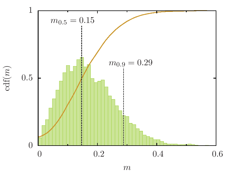
Figure 1.— Test of the Einstein@Home stochastic template bank for the PMPS analysis. The green bars show a histogram of the mismatch distribution for 10 920 noise-free signals from simulated pulsars in circular orbits. The orange curve shows the cumulative distribution function (cdf) of the mismatch. The median $m_{0.5}$ and the 90%-quantile of the mismatch distribution $m_{0.9}$ are highlighted. The template bank covers 90% of the parameter space with mismatch $m<0.29$.

3.5. Searched Parameter Space

To conduct a blind search for new pulsars, we must decide what region of parameter space to cover with a template bank. With unlimited computing power, we could search any parameter space, no matter how large. In practice, the finite computing power of Einstein@Home dictates that we only search some part of the parameter space.

Our choice is motivated first by astrophysical reasons: to target Einstein@Home to an interesting range of putative pulsar spin frequencies and orbital parameters. Second, for practical reasons we decide to complete the Einstein@Home search on PMPS data within about a year, searching a previously unexplored part of the orbital parameter space. Thus we constrain the search parameter space by setting a probabilistic limit on projected orbital radii, and by an upper limit on spin frequencies.

We estimated the available computing resources based on small-scale tests on a single computer and on the Atlas computing cluster at the AEI. The total Einstein@Home computing power was estimated from previous searches for radio pulsars.

The required number of orbital templates grows $\propto f_{\text{max}}^{3}$. We constrained our orbital template bank to $f_{\text{max}}=130$ Hz ($P_{\text{min}}\approx 7.7$ ms).

Standard acceleration searches lose sensitivity where $P_{\text{orb}}\lesssim 10T$. As discussed in Sec. 2, previous searches (Eatough et al., 2013) were sensitive for orbital periods $P_{\text{orb}}\lesssim 3$ hrs. Thus we searched for orbital periods in the range $86\text{\,min}\leq P_{\text{orb}}\leq 317\text{\,min}$. The upper boundary was chosen to provide seamless connection to the sensitivity ranges covered by previous searches. The lower boundary was dictated by the available computing power. Sensitivity to orbital periods as short as 86 min significantly increases the sensitivity to pulsars in compact binaries. We added a single template corresponding to an isolated pulsar to sustain sensitivity to isolated pulsars, or those in very wide orbits.

To provide full sensitivity along the complete orbit of any putative binary pulsar, the initial orbital phase $\psi$ was not constrained, covering the range $0\leq\psi<2\pi$.

We constrained the projected orbital radius by using a probabilistic bound on the orbital inclination angles based on the masses of putative pulsars and companions. From Kepler’s third law we define

$$0\leq a\sin(i)\leq\alpha\frac{G^{\frac{1}{3}}\Omega_{\text{orb}}^{-\frac{2}{3}}m_{\text{c,max}}}{c(m_{\text{p,min}}+m_{\text{c,max}})^{\frac{2}{3}}},$$ (4)

where $m_{\text{c,max}}$ is the maximum companion mass, $m_{\text{p,min}}$ is the minimum pulsar mass, $G$ is the gravitational constant, and $c$ is the speed of light. The constant $\alpha$ measures the probabilistic bound on orbital inclination angles. For our search, we chose $\alpha=0.5$, $m_{\text{p,min}}=1.2$ M_⊙ and $m_{\text{c,max}}=1.6$ M_⊙. The scaling of the total number of templates with $\alpha$, the pulsar and companion masses and the orbital period range is non-trivial.

For different pulsar and companion masses, Eq. (4) defines an upper limit on projected orbital radii as a function of the orbital angular velocity. For large companion masses, only a fraction of all possible orbital inclinations fulfill (4). In other words: for smaller companion masses, the condition (4) is fulfilled for any $i$, and all of such binary pulsar systems are detectable by Einstein@Home.

Fig. 2 shows the slice of orbital parameter space defined by these conditions. This choice guarantees that circular orbits at mass ratios for almost all pulsar-white dwarf binaries and many double neutron star systems lie inside our search space.

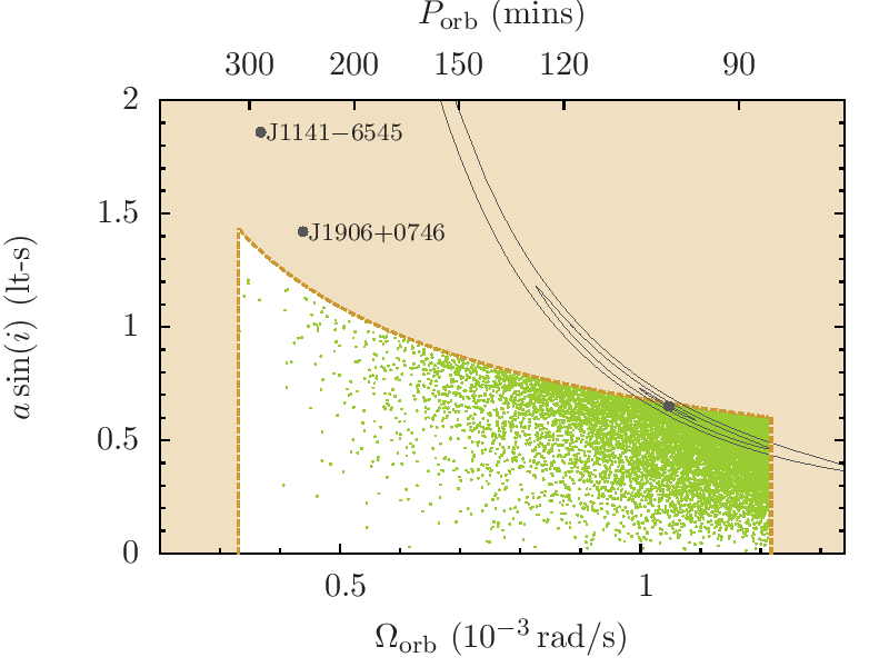
Figure 2.— The positions of the orbital templates (green dots) in the stochastic template bank constructed for this search. The parameter space we searched is shown in white, limited by the orange dashed line. The templates shown here are constructed at $f_{\text{max}}=130$ Hz. Dark-gray lines show cuts at $\psi=0$ through surfaces of constant mismatch $m=0.3$ around a single template (dark-gray dot) at orbital parameters $P_{\text{orb}}=100$ min, $a\sin(i)=0.65$ lt-s, and $\psi=0$. We chose signals at spin frequencies $f$ of 130 Hz, 65 Hz, and 15 Hz, respectively. Note that at lower frequencies the enclosed area extends far beyond the parameter space covered by the templates, enabling discoveries outside the parameter space. Known binaries are shown as labeled dark-gray dots.

Because we use the same template bank for all spin frequencies, it ‘over-covers’ the parameter space for frequencies $f<f_{\text{max}}$. The required density of templates is highest at $f_{\text{max}}$, because the detection statistic depends upon the difference in phase, which varies most rapidly at the highest frequency. For frequencies higher than $f_{\text{max}}$, it ‘under-covers’ the parameter space. In Fig. 2, we show cuts through surfaces of constant mismatch around a single template with fixed orbital parameters and varying spin frequency. At lower frequencies, the region covered by the templates is “banana-shaped” and extends well beyond the parameter space boundaries defined above. This is why our search detected the relativistic pulsar J1906$+$0746 (see Sec. 3.8) although its orbital parameters lie outside the parameter space covered by our template bank.

Our search loses sensitivity to the higher harmonics of fast-spinning MSPs, and searching for these higher harmonics is prohibited by the high computing costs. Increasing the value of $f_{\text{max}}$ to (say) 1 kHz, is computationally unfeasible and would require $\approx 500$ times more computing resources than our search!

3.6. Comparison to Standard Searching

As discussed in Sec. 3.5, standard acceleration searches (Ransom et al., 2002) lose sensitivity for binary pulsars with $P_{\text{orb}}\lesssim 10T$. To quantify this effect for the PMPS data, we numerically computed the mismatch of an acceleration search and that of the Einstein@Home search at different orbital parameter space points and at the highest spin frequency $f_{\text{max}}=130$ Hz. The orbital parameter space was covered by a cubic grid of 10 920 points in $\Omega_{\text{orb}}$, $a\sin(i)$, and $\psi$.

For each of the orbital parameter space points, we numerically simulated an acceleration search and the Einstein@Home search for a signal at this point. The simulated acceleration search followed the standard setup (Lorimer & Kramer, 2005): We set up a grid of accelerations $a_{1}$ in a range of $\pm 500$ m s^-2 and in steps of $\delta a_{1}=0.26$ m s^-2. The acceleration range was chosen to agree with Eatough (2009), and the acceleration step size was chosen (very conservatively) requiring that the signal does not drift by more than half a Fourier bin as described in Sec. 6.2.1 of Lorimer & Kramer (2005). Further, we simulated the same frequency resolution $\Delta f=1/(3T)$ as for the Einstein@Home search. Then, we generated noise-free sine-wave signals given by Eq. (1), and computed the detection statistic $\mathcal{P}_{1}=S_{0}$, but using a template phase model $\Phi(t)$ which is a quadratic function of $t$, corresponding to the signal from a single-harmonic isolated pulsar moving with constant acceleration.

For the simulated Einstein@Home search, the detection statistic $\mathcal{P}_{1}=S_{0}$ was computed using a template phase model from Eq. (1), then the fractional loss of detection statistic (mismatch $m$) was computed for both the acceleration and the Einstein@Home search.

Fig. 3 shows the results of our comparison, where we have averaged the mismatch over the orbital phase $\psi$. For the simulated Einstein@Home search (left panel), the averaged mismatch $\overline{m}$ is close to the target value of nominal mismatch ($m_{0}=0.3$) in the entire parameter space. Because of the underlying random template bank, there are small parts with slightly higher and lower mismatches. Close to $a\sin(i)=0$, the mismatch is considerably smaller, since this parameter space region is covered by the single template for isolated pulsars.

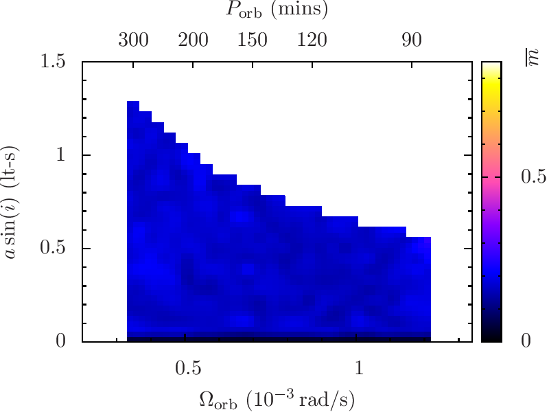
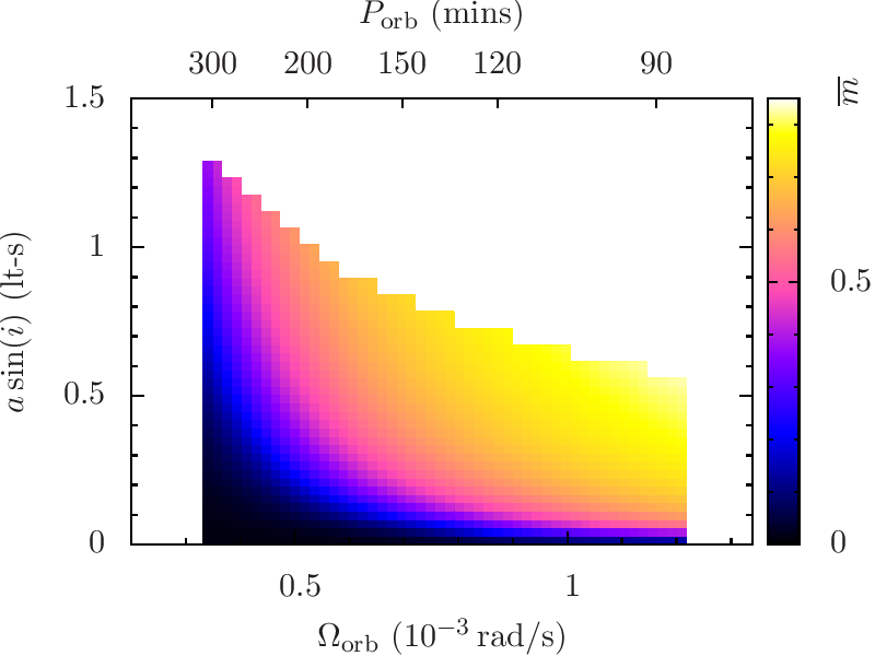
Figure 3.— Comparison of the mismatch in the Einstein@Home processing (left) and an acceleration search (right). (Left) The mismatch $\overline{m}$, averaged over $\psi$, computed on regularly spaced points in the space of $\Omega_{\text{orb}}$ and $a\sin(i)$. The grid consisted of 10 920 points, in each of which a sine-wave noise-free signal was generated and searched for with the complete stochastic template bank. The coverage is not uniform, because the stochastic template bank is based on random template banks. (Right) The results of a simulated acceleration search over the same parameter space grid. Note the significant loss of sensitivity of the acceleration search for higher values of $\Omega_{\text{orb}}$ and $a\sin(i)$.

For the simulated acceleration search (right panel of Fig. 3), the mismatch reaches unacceptably high values $\overline{m}\gtrsim 0.5$ over a large fraction of the parameter space. Only in a small part does the acceleration search achieve mismatches comparable to the our method. Our results clearly show the improvement in the detection of radio pulsars in compact binary orbits. Regions of signal parameter space that were virtually inaccessible with acceleration searches are in reach of our method.

3.7. Analysis on the Einstein@Home Host Machines

This section summarizes the “signal analysis” part of the Einstein@Home radio pulsar search pipeline, which runs on the volunteers’ hosts and does the bulk of the computing work. The code is distributed under the GPL 2.0 license and is available for CPUs and GPUs under Linux, Windows, and Mac OS X; a complete description may be found in Allen et al. (2013).

For each host, the input data are typically four de-dispersed time series which are analyzed sequentially as described here. The search code computes the detection statistics $S_{0},\dots,S_{4}$ at each template-bank point in parameter space, and then returns back to the Einstein@Home server a list of “top candidates”: the points in parameter space where the detection statistic was largest. The analysis consists of a data preparation step, a loop over orbital templates, and an output/candidate reduction step.

In the data preparation step, the input time series is uncompressed and converted into single-precision floating-point format. It is whitened in the frequency domain using a running-median average spectrum. RFI is replaced by computer-generated Gaussian noise using a list of known contaminated frequency bands in the fluctuation power spectra of the zero-DM de-dispersed PMPS data (Faulkner et al., 2004); this “zapping” step uses same list globally for the analysis of all PMPS beams. After this whitening and cleaning, the data are returned to the time-domain.

Then the search code begins to iterate through the orbital templates. For each orbital template, the detection statistics $S_{0},\dots,S_{4}$. of Eq. (2) are computed on the full frequency grid with spacing $\Delta f=1/3T$. This is done by resampling the data in the time-domain to remove the effects of the orbital modulation. The data are then mean-padded to length $3T$ and Fourier transformed using a fast Fourier transform (FFT); the detection statistic $\mathcal{P}_{n}$ is the squared modulus of the Fourier amplitude of the resampled time series in the $n$th frequency bin.

Inside the loop, the client search code maintains five different lists of candidates corresponding to the detection statistics $S_{0},\dots,S_{4}$. Each contains the 100 candidates with the largest values of $S_{i}$ having distinct values of fundamental frequency $f$. The code checkpoints after each loop iteration; if needed this permits it to be restarted with little loss of compute time.

When the loop over orbital templates is complete, the statistical significance $\mathcal{S}$ is computed for all 500 candidates, and the 100 with the highest $\mathcal{S}$ are returned to the Einstein@Home server in a single result file. Based on false-alarm statistics one can show that selecting the 100 most significant candidates results in digging down well into the noise-dominated regime.

The result file is uploaded to the central Einstein@Home servers and validated in a two-step process, described in Allen et al. (2013). In order to be accepted it has to agree with the result calculated by another volunteer’s computer with a fractional accuracy of about one part in $10^{5}$.

3.8. Manual Candidate Selection

After the upload of all 440 result files for each beam, one has to filter out the most promising candidates from all 44 000 candidates in each beam. The majority of candidates in any given beam are caused by random noise fluctuations and have low significance values $\mathcal{S}$. Thus, thresholding on $\mathcal{S}$ is a possible step in reducing the number of candidates. However even in the presence of a highly-significant signal, correlations can cause the signal to show up at multiple DMs, frequencies, and/or orbital parameters. Thus, more sophisticated methods are required to reduce the number of candidates to follow up.

We used two methods to identify pulsar-like signals, employing frequency coordinates tailored to the binary parameter space. One method is based on producing overview plots that allow a quick and easy identification of pulsars and first estimates of their orbital parameters. The second method employs automated filtering algorithms to identify promising candidates in the binary parameter space. Fig. 4 shows a flow diagram comparing both methods, which we describe in the following.

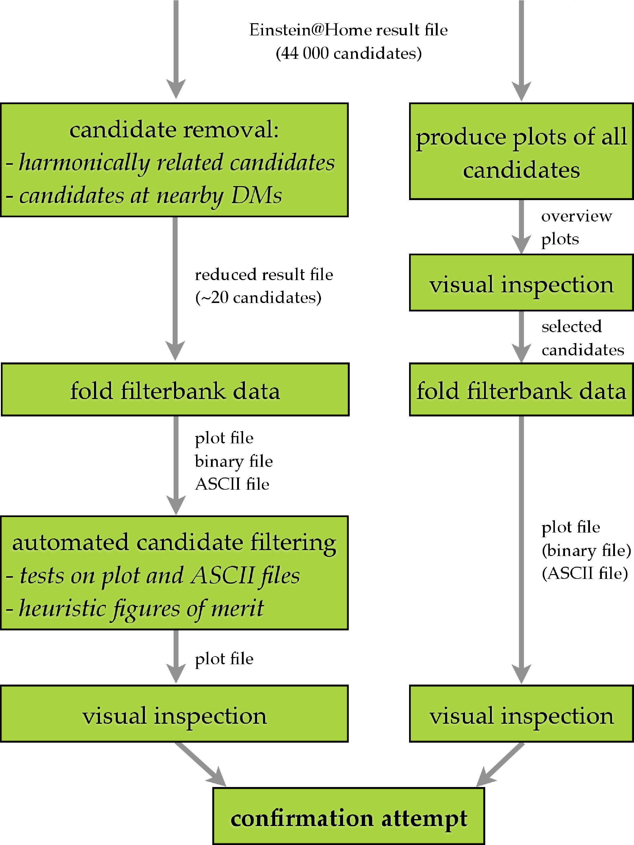
Figure 4.— Turning the Einstein@Home results into confirmations of new pulsars: this diagram shows the steps of the two post-processing methods used in our search. The right-hand side displays the methods using the visual inspection of overview plots described in Sec. 3.8. The left-hand side shows the steps of the automated post-processing methods to reduce the number of candidates from Sec. 3.9.

Our first method for the identification of promising pulsar candidates in the Einstein@Home result files uses custom-made overview plots. These visualize the complete set of candidates for any given PMPS observation. We identified pulsars by characteristic patterns in these plots. Promising candidates are followed up with tools from the presto software suite.

The set of overview plots is automatically produced for visual inspection when all valid result files for a given beam are available on the Einstein@Home servers. The plots show the significance for all 44 000 candidates as a function of a the spin frequency at the detector $\nu_{1}$, the associated spin frequency derivative $\nu_{2}$, and combinations of the orbital template parameters. The coordinates $\nu_{1}$ and $\nu_{2}$ resolve some of the correlations of the detection statistic $\mathcal{P}_{n}$ in the orbital parameters. The $\nu_{1}$ and $\nu_{2}$ are the linear and quadratic coefficients in a polynomial expansion of the phase model (1) in $t$. Their derivation may be found in the Appendix.

An example of the five different plots in our post-processing is given in Fig. 5, which shows the highly-significant detection of the binary pulsar J1906$+$0746 in the Einstein@Home results.

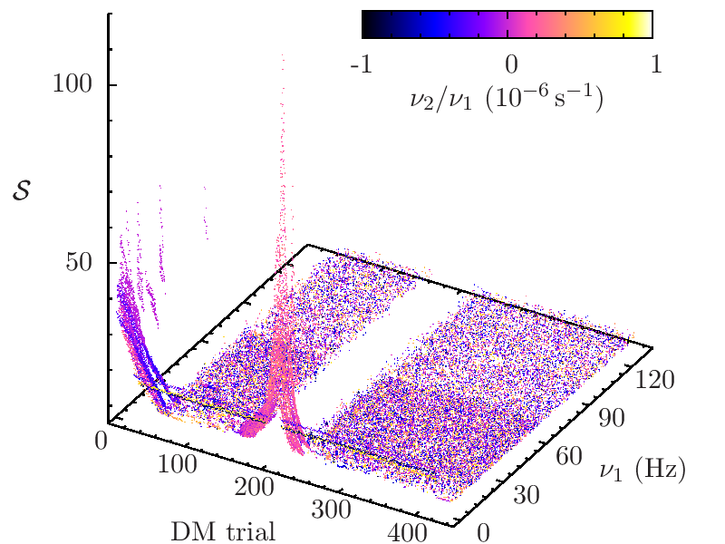
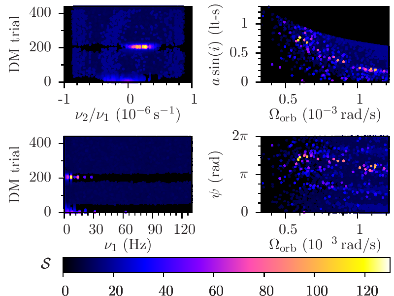
Figure 5.— Example post-processing overview plots, showing the highly-significant detection of the binary pulsar J1906$+$0746. (Left) The plot shows the significance $\mathcal{S}$ as a function of the DM trial number and the spin frequency $\nu_{1}$ at the detector of each candidate. The color code displays the relative change in spin frequency $\nu_{2}/\nu_{1}$ from orbital motion. The coordinates $\nu_{1}$ and $\nu_{2}$ are the first two coefficients of the polynomial expansion of the orbital phase as given in the Appendix. Since the top 100 candidates are reported for each DM trial and the pulsar is detected with very high significance, there are no detections of the noise floor in a DM range around the pulsar. The missing noise floor at low DM is caused by remnant RFI discernible by increasing $\mathcal{S}$ towards $\text{DM}=0$ pc cm^-3. (Right) The four sub-panels show the significance $\mathcal{S}$ in color-code as a function of different combinations of spin frequency and the orbital parameters. The top left shows $\mathcal{S}$ projected onto the space of relative frequency change $\nu_{2}/\nu_{1}$ and DM trial number, the top right plot shows $\mathcal{S}$ in the space of orbital angular velocity $\Omega_{\text{orb}}=2\pi/P_{\text{orb}}$ and projected orbital radius $a\sin(i)$. The bottom left plot displays $\mathcal{S}$ as a function of spin frequency $\nu_{1}$ and DM trial number, the bottom right plot shows $\mathcal{S}$ in the space of orbital angular velocity $\Omega_{\text{orb}}$ and initial orbital phase $\psi$. Note the clearly visible non-zero value of $\nu_{2}/\nu_{1}$ caused by the orbital motion of the pulsar in its 4-hr orbit during the 35 min observation. Even though only about 15% of its orbit was observed, the right-hand side panels already allow some first constraints of the orbital parameters.

The number of candidates identified from these overview plots is relatively small (a few per beam at most, none in the majority of beams, and on average one candidate in $\sim 50$ beams). Tools from the presto software suite are used to fold the full-resolution filterbank data at the candidate spin period and DM identified from the Einstein@Home results and to optimize the parameters. In total we inspected of order 1000 of these folded time series plots by eye and used them to judge the broadband nature and temporal continuity of the signal. The ATNF catalogue (Manchester et al., 2005), and Web sites listing known, but as yet unpublished, pulsars are checked to ensure that the candidate is not a detection of a known pulsar. About half of our new discoveries were found by the visual inspection of overview plots.

3.9. Automated Candidate Selection

The visual inspection of overview plots is augmented by an automated post-processing stage. This sifts through all candidates in a given beam and identifies the most promising ones for a follow up via folding of the filterbank data. With infinite computing and man power, all candidates of a given beam would be used for folding the filterbank data. In practice, this is neither feasible nor necessary. Folding the 44 000 candidates for any given beam requires an unfeasibly large amount of computing time and human resources for further inspection. Many of the candidates will be caused either from random noise or by a single pulsar (or RFI) signal. For example, following up candidates at harmonically related frequencies and nearby DM trials does not yield additional information (c.f. Fig. 5).

The first goal of the automated post-processing is to reduce the number of candidates from the complete results files. The second goal is to find those pulsars whose identification with the overview plots is difficult. Weak signals at higher spin frequencies may only be registered at a few trial DMs above the noise level, making it difficult to detect them visually.

The automated post-processing consists of three steps. In the first step we reduce the number of harmonically related candidates. We start at the candidate with the highest value of $\mathcal{S}$. Candidates associated with sub-harmonic and harmonic frequencies of this candidate are flagged as possibly related as follows. We conservatively assume a frequency band around the candidate’s value of $\nu_{1}$ with a width $\delta\nu_{1}$ given by the maximum Doppler modulation of all templates in the orbital template bank. The width of the frequency band is obtained from maximizing the frequency modulation amplitude $\Omega_{\text{orb}}a\sin(i)/c$ over the entire orbital template bank and computing the Doppler range at frequency $\nu_{1}$ from

$$\delta\nu_{1}=\nu_{1}\max(\Omega_{\text{orb}}a\sin(i)/c).$$ (5)

After this step, only candidates in the Doppler range around the fundamental frequency are retained for the next step.

These are further winnowed down in the second step. Real pulsar candidates should produce a peak in significance as a function of DM, separated from the noise-dominated background. To take this property into account, we approximate the significance as a function of DM (Cordes & McLaughlin, 2003) by a parabola

$$\mathcal{S}(\text{DM})=\mathcal{S}_{0}\left(1-\frac{\text{DM}-\text{DM}_{0}}{\Delta\text{DM}}\right)^{2}.$$ (6)

Here, $\mathcal{S}_{0}$ is the significance of the most significant candidate at central dispersion measure $\text{DM}_{0}$, and $\Delta\text{DM}$ is the “width” of the parabola, such that $S(\text{DM}_{0}\pm\Delta\text{DM})=0$.

Now, we step over a fixed grid of ten trial values of $\Delta\text{DM}$ between 0.6 pc cm^-3 and 50 pc cm^-3 and determine the best-fit parabola parameter $\Delta\text{DM}$, i.e. the one with the smallest squared residuals. To make sure that the parabola approximation is accurate, we select candidates near the top of the peak with $\mathcal{S}\geq 0.6\mathcal{S}_{0}$. Out of all candidates within the Doppler frequency range and the best fitting DM range we only keep the most significant candidate.

The procedure of removing harmonically related candidates and those at similar DMs described above is iterated with the next most significant candidate until only “independent” candidates are left.

The number of remaining candidates per beam was about 20 after this first reduction step. We then folded all reduced candidates using the presto software on the Atlas cluster at the AEI. Each candidate was folded at fixed DM with five different spin frequencies between $\nu_{1}-2\delta\nu$ and $\nu_{1}+2\delta\nu$. Here, $\delta\nu$ is the expected Doppler shift in spin frequency caused by orbital motion and is computed from the orbital parameters of the candidate. Folding at a conservatively wide parameter range accommodates possible offsets from the true orbital parameters. In this step, we folded of order 4 000 000 candidates for the whole PMPS search. Due to oversight, we folded the original data, not the ones resampled at the orbital parameters. We will re-run our post-processing and report results in a future paper.

The final step of our automated post-processing is done by an algorithm implemented in idl, which selects pulsar-like candidates based on figures of merit derived from the prepfold plots and associated binary and ASCII files.

The algorithm first checks for disqualifying metrics in the ASCII file associated with the folded data output. Features that cause rejection include periods that fall within the range of known interference signals and a signal strength below a chosen threshold (5.0$\sigma$ as computed by prepfold).

For output files that survive these tests, the software uses two different tests applied directly to the plots produced by prepfold. It applies them separately to two parts of each plot, see e.g. Fig. 7. The first test looks for signal strength and consistency in phase in the time versus phase plot (left hand bottom subplot in Fig. 7). A pulsar-like signal is a straight, vertical line when folded with the proper parameters. An average intensity is computed for each vertical line at every horizontal phase position by summing the pixel values in that column and dividing by the number of pixels summed. A pixel smoothing of 3, 9, and 21 phase bins is applied in the phase (horizontal) direction prior to taking each sum. This smoothing accounts for different possible pulse widths. The resulting average intensity values for the vertical columns are then compared to with an off-pulse average intensity value, and a different threshold test is applied for each smoothing case.

A second test looks at a contour plot showing signal strength as a function of trial period and period derivative (bottom right sub-plot in Fig 7). The expected signal is one that is localized with one significant peak. The algorithm counts and classifies the number of consolidated strong response regions (determined by the number of contiguous pixels that are saturated) into “large” and “small” areas, which have sizes of at least 8 and 250 pixels, respectively. These correspond to 0.03% and 0.86% of the total area of the bottom right sub-plot in Fig 7. The code retains the candidate as valid if one or two large areas and no more than 13 total large and small areas are counted, or if there are less than eight total large and small areas (regardless of the number of large areas). Violation of either of these conditions indicates that the plot is not likely to reflect a unique period and period derivative combination. Testing for both small and large areas was chosen to account for the fact that not all pulsar signals will be strong enough to yield just a single contour peak.

The thresholds described above were chosen by using a subset of the PALFA data collected with the WAPP backends (Cordes et al., 2006) as a test case. A variety of area sizes and threshold numbers were tried for the tests to optimize the results (that is, until the number of candidates passing the test was reduced as much as possible without eliminating any known pulsars).

The idl code reduces the number of candidates by up to a factor of a hundred, leaving a number ($\sim 100\,000$) that we individually checked by eye.

Our two different pulsar identification methods have different selection effects, making them sensitive to different classes of pulsars. The automated processing has proven very useful in identifying signals which were missed in the overview plots, because they were weak and/or masked by RFI (cf. Tab. 2). But, since visual inspection of result plots and human judgment is the final step in both methods, human error is a possible source for the rejection of real pulsar signals. The simplified folding at five different spin frequencies as described above can lower the sensitivity to the most extreme compact binary pulsars in the automated candidate selection.

4. Einstein@Home Discoveries in the PMPS Data

Any pulsar candidate surviving the checks described above was scheduled for re-observation to confirm the celestial nature of the candidate signal. We confirmed the pulsar discoveries presented here using the Parkes telescope, the Lovell telescope at Jodrell Bank, and the Effelsberg telescope. After the initial discovery, regular timing observations were conducted to further characterize the pulsar and a possible binary system. All timing solutions presented in this publication were obtained with observations at the Lovell telescope.

In total, 24 previously unknown pulsars have been identified. Most of the new discoveries are relatively faint, with period-averaged flux densities between 0.1 mJy and 2.7 mJy at 1.4 GHz. The spin periods of the discoveries lie between 3.78 ms and 2624 ms. Eighteen pulsars are isolated, and six are members of binary systems.

Follow-up observations at Jodrell Bank used a dual-polarization cryogenic receiver on the 76-m Lovell telescope, having a system equivalent flux density of 25 Jy. Data were processed by a digital filterbank which covered the frequency band between 1350 MHz and 1700 MHz with channels of 0.5 MHz bandwidth. We typically made observations with a total duration of between 10 min and 40  min, depending upon the discovery signal-to-noise ratio. Data were folded at the nominal topocentric period of the pulsar for sub-integration times of 10 s. After inspection and ‘cleaning’ of any RFI, we de-dispersed profiles at the nominal value of the pulsar DM. Initial pulsar parameters were established by conducting local searches in period and DM about the nominal discovery values and finally summed over frequency and time to produce integrated profiles. Time of arrival (TOA) data were obtained after matching with a standard template and processed using standard analysis techniques with psrtime and tempo.

In the following, we present all 24 discoveries. Tab. 2 shows the properties of all new pulsars from our search. For pulsars without a coherent timing solution, the sky position was derived from the discovery beam center coordinates or weighted averages in case of detections in multiple beams. The position error is given by the PMPS beam size. The spin period $P$ for pulsars without coherent timing solution is from the discovery observation. We calculated the flux densities $S_{1400}$ from the discovery observations using the radiometer equation, e.g. (Lorimer & Kramer, 2005) with the gain and system temperature of the Parkes 21-cm Multibeam Receiver (Staveley-Smith et al., 1996). The DM is the nominal value from the discovery observation. The distance $D$ was estimated based on a Galactic electron density model from Cordes & Lazio (2002) with typical errors at the level of $\sim$20%. For reproducibility of our results, we quote the discovery PMPS beam and the Einstein@Home significance $\mathcal{S}$ from Eq. (3). The last column shows the discovery method, either ‘V’ for the visual inspection of overview plots, or ‘A’ for the automated post-processing. A total of 13 pulsars were found by the first method, the remaining 11 by the second method. We have found coherent timing solutions for five of our discoveries, marked in the table with ^†.

Table 2Pulsars discovered by the Einstein@Home analysis of the Parkes Multi-beam Pulsar Survey data. Sources with a fully-determined timing solution are marked with ^† and pulsars in binary systems by ^♭. For these sources, the values in parentheses are the 1-sigma errors as reported by tempo. For pulsars without a coherent timing solution, right ascension (RA) and declination (Dec) are the beam center coordinates or weighted averages in case of detections in multiple beams. Their position error is estimated from the PMPS beam size. Their spin periods $P$ and dispersion measure DM are the values in the discovery observations. $S_{1400}$ denotes flux densities and $D$ the estimated distance. The discovery PMPS beam and the Einstein@Home significance $\mathcal{S}$ are given for reproducibility reasons. The last column shows the discovery method: ‘V’ for the visual inspection, or ‘A’ for the automated method.

PSR	RA	Dec	$P$	$\dot{P}$	$P$ Epoch	DM	$S_{1400}$	$D$	PMPS beam	$\mathcal{S}$
	(J2000)	(J2000)	(s)	$\left(10^{-15}\right)$	(MJD)	(pc cm-3)	(mJy)	(kpc)
J0811$-$38	08:11.7(5)	$-$38:57(7)	0.482594(2)	–	50824.5	336.2	0.3	6.2	0026_0051	15.6	V
J1227$-$6208♭	12:27.6(5)	$-$62:10(7)	0.034529685(8)	–	51034.1	363.2	0.8	8.4	0058_036D	17.9	A
J1305$-$66	13:05.6(5)	$-$66:39(7)	0.1972763(2)	–	51559.7	316.1	0.2	7.5	0109_0033	15.5	A
J1322$-$62	13:22.9(5)	$-$62:51(7)	1.044851(4)	–	50591.6	733.6	0.3	13.2	0001_0016	23.1	V
J1455$-$59	14:55.1(5)	$-$59:23(7)	0.1761912(2)	–	50841.7	498.0	1.6	7.0	0038_0182	14.0	V
J1601$-$50	16:01.4(5)	$-$50:23(7)	0.860777(4)	–	50993.6	59.0	0.4	3.6	0042_0039	29.1	A
J1619$-$42	16:19.1(5)	$-$42:02(7)	1.023152(4)	–	51975.6	172.0	0.6	3.7	0137_041B	35.4	V
J1626$-$44	16:27.0(5)	$-$44:22(7)	0.3083536(5)	–	51718.6	269.2	0.3	4.8	0125_077C	13.2	A
J1637$-$46	16:37.6(5)	$-$46:13(7)	0.493091(2)	–	50842.9	660.4	0.7	7.0	0039_0055	17.2	V
J1644$-$44	16:44.6(5)	$-$44:10(7)	0.1739106(2)	–	51030.2	535.1	0.4	6.2	0056_020B	14.1	V
J1644$-$46	16:44.1(5)	$-$46:26(7)	0.2509406(1)	–	50839.0	405.8	0.8	4.8	0035_0293	13.2	A
J1652$-$48♭	16:52.9(5)	$-$48:45(7)	0.0037851238(4)	–	51373.3	187.8	2.7	3.3	0085_0254	22.3	A
J1726$-$31♭	17:26.6(5)	$-$31:57(7)	0.12347018(9)	–	51026.4	264.4	0.4	4.1	0054_015A	15.9	A
J1748$-$3009♭	17:48:23.79(2)	$-$30:09:12.2(5)	0.009684273(2)	–	51495.1	420.2	1.4	5.0	0102_0059	18.0	A
J1750$-$2536♭	17:50:33.39(2)	$-$25:36:43(3)	0.034749053(8)	–	50593.8	178.4	0.4	3.2	0002_0089	15.9	A
J1755$-$33	17:55.2(5)	$-$33:31(7)	0.959466(4)	–	52080.6	266.5	0.2	5.7	0141_0097	21.2	V
J1804$-$28	18:04.8(5)	$-$28:07(7)	1.273011(9)	–	51973.7	203.5	0.4	4.2	0137_039B	13.2	A
J1811$-$1049†	18:11:17.07(8)	$-$10:49:03(4)	2.6238585620(3)	0.8(2)	55983.5	253.3	0.3	5.5	0149_0108	29.2	V
J1817$-$1938†	18:17:06.82(8)	$-$19:38.6(2)	2.0468376289(2)	0.36(9)	55991.8	519.6	0.1	8.6	0011_0323	16.9	V
J1821$-$0331†	18:21:44.70(3)	$-$03:31:12.7(1)	0.90231562918(4)	2.53(2)	55980.9	171.5	0.2	4.3	0148_0197	28.3	V
J1838$-$01	18:38.5(5)	$-$01:01(7)	0.1832948(2)	–	51869.1	320.4	0.3	6.9	0132_0627	16.7	V
J1838$-$1849†	18:38:33.79(4)	$-$18:49:59(5)	0.48824200896(3)	0.04(1)	55991.9	169.9	0.4	4.5	0140_0064	31.7	V
J1840$-$0643♭†	18:40:09.44(5)	$-$06:43:47(1)	0.0355778755(3)	0.2202(7)	55930.0	500.0	1.2	6.8	0060_0206	18.2	V
J1858$-$0736	18:58:44.3(7)	$-$07:37(7)	0.551058591(2)	5.06(7)	56108.5	194.0	0.3	5.0	0143_0051	16.7	A

To compare our discoveries with the known population, we show DM and spin periods of our discoveries, together with pulsars in the ATNF catalogue (Manchester et al., 2005) and those from earlier PMPS analyses (Manchester et al., 2001; Morris et al., 2002; Kramer et al., 2003; Hobbs et al., 2004; Faulkner et al., 2004; Lorimer et al., 2006; Keith et al., 2009; Keane et al., 2010; Mickaliger et al., 2012; Eatough et al., 2013) in Fig. 6. Most of our discoveries are at large DMs relative to the bulk of the ATNF pulsars, but their DM distribution agrees with that of other PMPS pulsars.

Notable are the discoveries at high DMs and small spin periods. This combination of DM and $P$ usually hampers the detection of pulsars, since the channel smearing increases with larger DMs and with smaller periods. Longer sampling times further decrease sensitivity to MSPs. Thus, the ratio $\text{DM}/P$ is a measure of how deep a survey probes the Galaxy for MSPs. Modern pulsar surveys thus compensate for these effects by narrow filterbank channels and short sampling times (Cordes et al., 2006; Keith et al., 2010). Given the 3-MHz wide channels and slow sampling time of 250 $\mu$s of the PMPS data, the discovery of pulsars like PSR J1652$-$48 and PSR J1748$-$3009 is surprising.

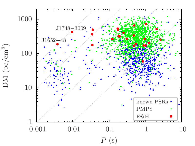
Figure 6.— Our discoveries in comparison with the known pulsar population in the Galactic field. The plot shows the DM vs. the period for all known pulsars–excluding sources in globular cluster and extra-galactic pulsars–from the ATNF catalog (blue triangles), discoveries from earlier PMPS analyses (green diamonds), and our new discoveries (red circles). The distribution of our discoveries at higher DMs is apparent, and agrees with the earlier PMPS discoveries. Notable are the discoveries of pulsars at lower spin periods and high DMs, especially that of PSR J1748$-$3009, the millisecond pulsar with the highest known DM. Dashed gray lines show points of $\text{DM}/P=\text{const}$, from top left to bottom right for $\text{DM}/P=50,10,1,0.1$ pc cm^-3 ms^-1.

Tab. 3 lists the orbital parameters of three newly discovered binary pulsars. Note that we have a coherent timing solution for only one of the sources. Improved orbital parameters and full timing solutions for the binary pulsars will be published in a followup article. Fig. 7 shows the discovery plots made with the presto tool prepfold for two selected pulsars, while Fig. 8 displays the discovery pulse profiles of all 24 sources. We describe notable sources in more detail below.

Table 3Orbital parameters of three binary pulsar systems discovered by the Einstein@Home analysis of the PMPS data.

PSR	data timespan	$a\sin(i)$	$e$	$T_{0}$	$P_{\text{orb}}$	$\omega$	Epoch
	(MJD)	(lt-s)		(MJD)	(d)	(degs)	(MJD)
J1748$-$3009	56055 – 56174	1.32008(1)	–	56069.162075(7)	2.9338198(4)	–	51495.13
J1750$-$2536	56036 – 56176	20.06096(5)	0.000392(4)	56069.27(3)	17.141650(4)	54.7(7)	50593.78
J1840$-$0643	55699 – 56161	113.2(2)	–	56044.4(1)	937.1(7)	–	55930.01

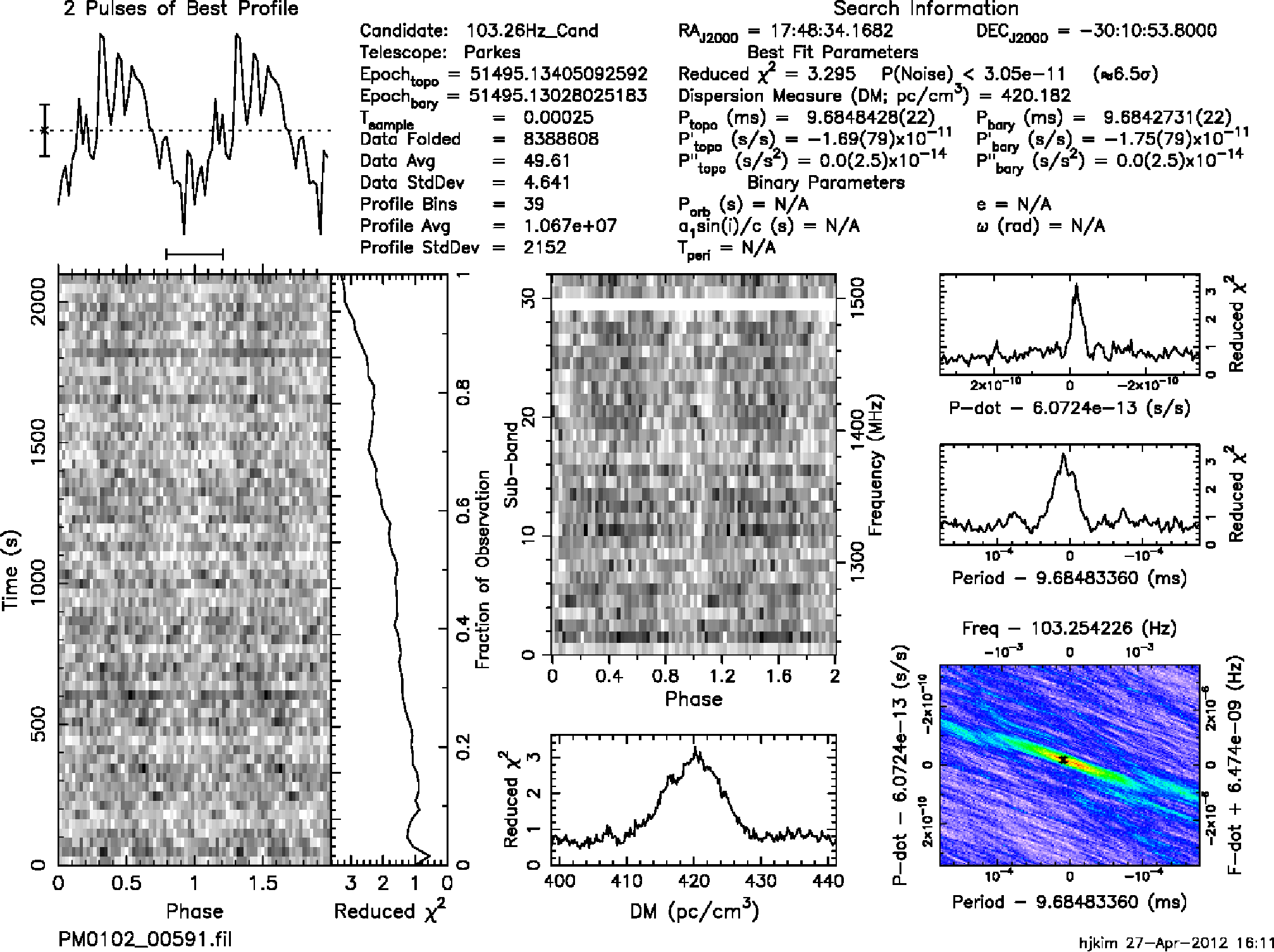
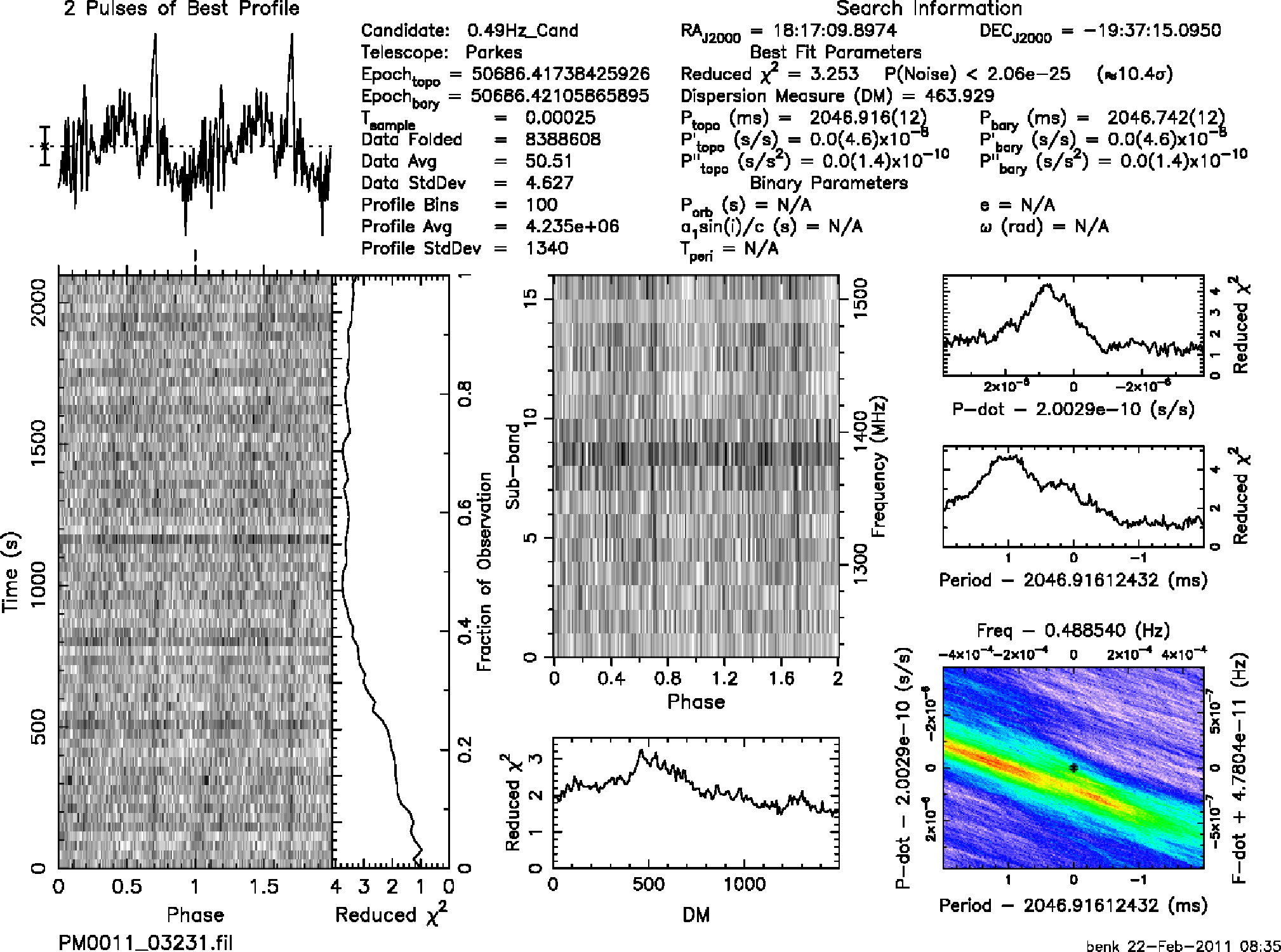
Figure 7.— presto discovery plots for two of the 24 pulsars found by Einstein@Home in the PMPS data. (Left) The discovery plot of the millisecond pulsar J1748$-$3009. Its pulse profile is very wide and appears almost sinusoidal from smearing over the 3 MHz wide filterbank channels used in the PMPS. (Right) The discovery plot of the slow pulsar J1817$-$1938, which exhibits clear signs of intermittency. Its emission gradually disappears towards the middle of the 35 min observation. Note also that the pulsar was discovered in our search despite the much stronger RFI at nearby periods, which is clearly visible. This discovery plot shows a slight phase-drift because it was folded with a small frequency offset.

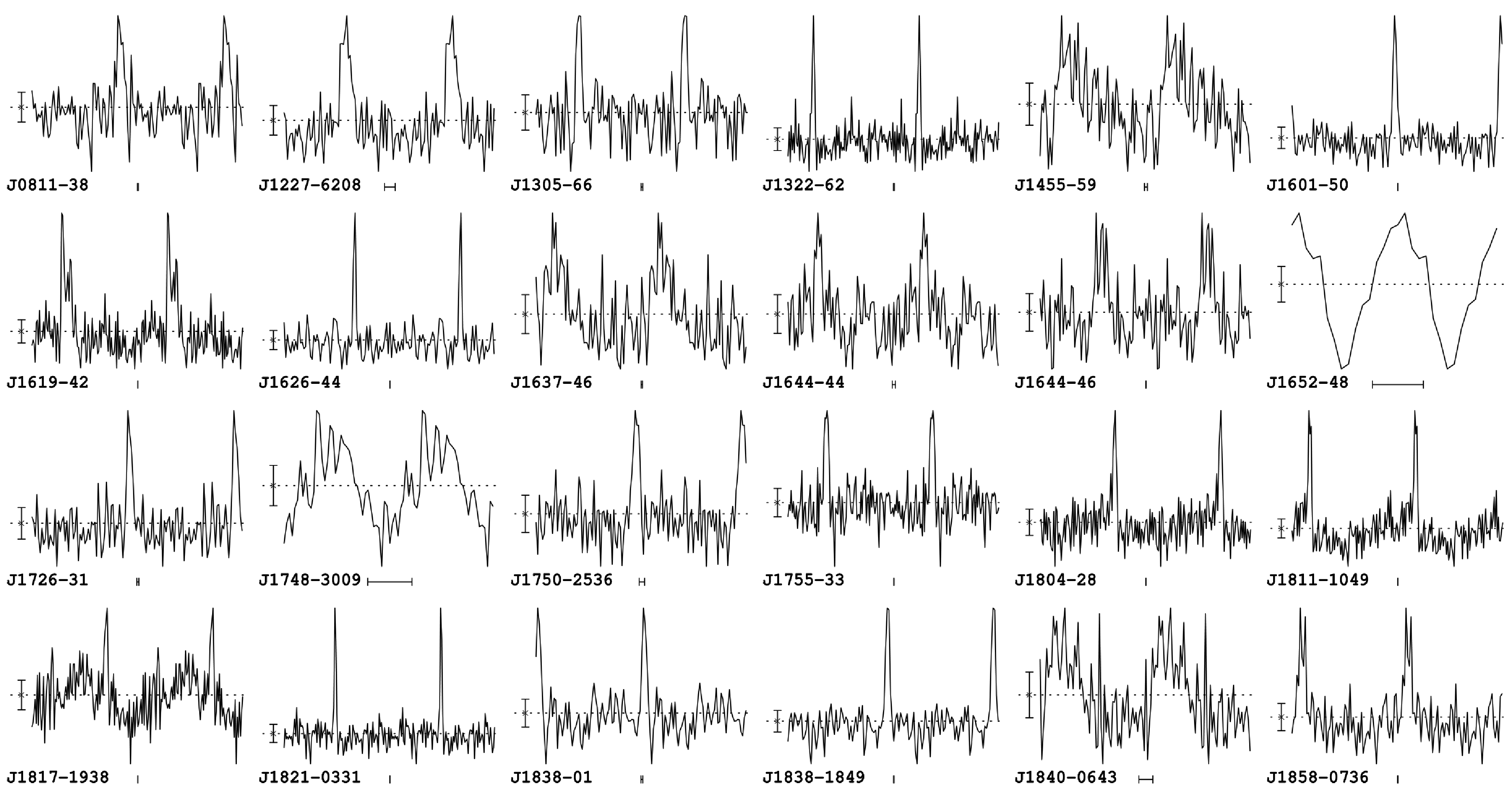
Figure 8.— Discovery pulse profiles for all 24 pulsars. Each panel shows the flux density over two rotations of the pulsar, is based on a single 35 min observation from the PMPS, and has been folded with prepfold. On the left side of each profile is a vertical bar showing the standard deviation of the noise baseline, and on the bottom is a horizontal bar showing the time resolution in the profile. Note the almost sinusoidal pulse profiles of PSR J1652$-$48 and PSR J1748$-$3009, which are strongly affected by filterbank channel smearing. The pulse profile of PSR J1455$-$59 shows a pronounced multi-path scattering tail.

PSR J1227$-$6208

This pulsar in a binary system with a 6.7-day orbit was independently discovered by Mickaliger et al. (2012) and will be further characterized by Thornton et al. (in prep.). Although its significance $\mathcal{S}=17.9$ in the Einstein@Home pipeline is relatively high, it is rather inconspicuous in the overview plots because of strong remnant RFI. The automated post-processing successfully identified this pulsar.

PSR J1322$-$62

The discovery observation of this isolated 1045 ms pulsar at DM $\approx 734$ pc cm^-3 exhibits signs of intermittency. Follow-up observations confirmed this trend: we observed the pulsar three times at MJD 55592.7 ($T\approx 2100$ s), MJD 55615.7 ($T\approx 590$ s), and MJD 55648.6 ($T\approx 2100$ s), respectively, with the Parkes telescope. We only detected the pulsar in the second (shortest) observation. The non-detections in the two other observations correspond to upper limits on the flux density of $S\lesssim 0.07$ mJy, as computed from, e.g., Appendix 2.6 in Lorimer & Kramer (2005). Here, and for all following upper limits we assumed a signal-to-noise threshold of $8\sigma$, the observed pulsar duty cycle, sky temperature at the pulsar sky position and system parameters as given in, e.g., Manchester et al. (2001).

The pulsar apparently shows long-term nulling or intermittent emission behavior (Kramer et al., 2006a; Lorimer et al., 2012). Like the other intermittent pulsars presented here, their large inferred distances mean that interstellar scintillation is unlikely to be the cause of the observed intensity variations; at this observing frequency scintles of width of only a few MHz are expected and therefore average out over the 288 MHz band. Further observations are required to quantify this effect for PSR J1322$-$63.

PSR J1455$-$59

This isolated 176 ms pulsar showed a strongly pronounced scattering tail in its pulse profile in the discovery observation. Its DM $\approx 498$ pc cm^-3. Further measurements of the pulse shape at multiple radio frequencies could be used to study the interstellar medium, by determining exact values of the pulse-broadening time scales $\tau_{d}$. Assuming a delta-function pulse shape, we determine $\tau_{d}=0.08(4)$ s from the discovery observation. This is in very good agreement with the measurements in Bhat et al. (2004). More exact measurements of $\tau_{d}$ in turn can be used to improve Galactic electron density models (Cordes & Lazio, 2002), and to update existing empirical relations between $\tau_{d}$ and the DM (Bhat et al., 2004).

PSR J1652$-$48

This binary MSP has a spin period of 3.78 ms and a DM of $\approx 188$ pc cm^-3. This pulsar has the fifth highest value of DM$/P=49.7$ pc cm^-3 ms^-1 of all Galactic field pulsars. As discussed above, the ratio is a measure of the depth to which pulsar surveys probe our Galaxy for MSPs. The value for PSR J1652$-$48 is only surpassed by that for PSR J1903$+$0327, PSR J1900$+$0308, and PSR J1944$+$2236 found in the PALFA survey (Champion et al., 2008; Crawford et al., 2012), and by that for PSR J1747$-$4036, found through a radio search of an unidentified Fermi source (Kerr et al., 2012). The pulsar is being timed at the Parkes Observatory.

PSR J1726$-$31

We confirmed PSR J1726$-$31 upon the first re-detection attempt at Parkes telescope in 2012 February. In nine subsequent observations at Parkes, only one further detection of this pulsar at MJD 56111.5 has been made. The other non-detections were done with the following integrations times (upper limit on the flux density in parentheses): once with $T\approx 3600$ s ($S\lesssim 0.08$ mJy), four times with $T\approx 2100$ s, once with each $T\approx 1800$ s, $T\approx 1500$ s, and $T\approx 1300$ s ($S\lesssim 0.1$ mJy in each case). The large distance of 4.1 kpc, inferred from $\text{DM}\approx 264$ pc cm^-3 means interstellar scintillation is unlikely to be the cause of the observed intensity variations.

A search of the Parkes archival observation logs has revealed that this pulsar was independently identified as a promising candidate in 1999, at the time of the original PMPS observations. Four confirmation attempts were made in the same year, but without success. Three of them have integration times $T\approx 2100$ s and each limits the flux density to $S\lesssim 0.1$ mJy, one has $T\approx 360$ s and therefore $S\lesssim 0.25$ mJy.

Including our observations with these earlier confirmation attempts, and the original survey observation, the pulsar has been observed for a total of $\approx 8.6$ hr. Of this time the pulsar is visible for $\approx 1.9$ hr, suggesting the pulsar is detectable about 20 % of the time.

In addition to the intermittency, there is evidence for large period changes between observations, and one instance of significant line-of-sight acceleration ($a\approx 11$ m s^-2). This suggests that this pulsar is a member of a compact binary system. Additional timing observations to characterize this pulsar, its possible companion, and the orbital parameters are ongoing.

If this pulsar is in a compact binary system, it is strikingly similar to PSR J1744$-$3922 (Faulkner et al., 2004). PSR J1744$-$3922 is mildly recycled with a spin period of 172 ms (cf. 123 ms for PSR J1726$-$31) and resides in a compact binary system ($P_{\text{orb}}\approx 4.6$ hr). Like our discovery, PSR J1744$-$3922 also exhibits nulling and is visible for approximately 25 % of the time at 1.4 GHz.

PSR J1744$-$3922, and thus PSR J1726$-$31, might be the members of a new class of binary pulsars as proposed by Breton et al. (2007): these binary pulsars have long spin periods, large magnetic fields ($\sim 10^{10-11}$ G), low-mass companions, and low orbital eccentricities. Their evolutionary history is not well understood and known formation channels fail to explain all of their properties.

A different possible explanation for the observed intensity variations are eclipses in a compact binary systems: “black widow” systems like PSR B1957$+$20 (Fruchter et al., 1988). This seems unlikely, though, since the spin period of PSR J1726$-$31 is significantly larger than those of other known eclipsing binary pulsars (Freire, 2005).

PSR J1748$-$3009

This pulsar is a 9.7 ms pulsar in a 2.93 day binary orbit. With $\text{DM}\approx 420$ pc cm^-3 it has by far the highest DM of all MSPs known to date. Its value of DM$/P=43.3$ pc cm^-3 ms^-1 is the seventh highest value published (Manchester et al., 2005; Crawford et al., 2012). The pulsar is currently being observed at Jodrell Bank on a regular basis to determine a full timing solution, which we will publish in a second paper on our search. Tab. 3 shows first measurements of its orbital parameters. The mass function $f\approx 2.87\times 10^{-4}$ $M_{\odot}$ of this system indicates a minimum (median) companion mass of 0.09 $M_{\odot}$ (0.10 $M_{\odot}$) for a pulsar mass of 1.4 $M_{\odot}$.

PSR J1750$-$2536

This pulsar has a spin period of 34.7 ms and was discovered independently in two adjacent PMPS beams. It has a DM of $\approx 178$ pc cm^-3 and is a member of a binary system with an orbital period of 17.1 days. It is currently being observed regularly at Jodrell Bank to improve the timing solution, which will be published in a follow-up paper. Tab. 3 shows first measurements of its orbital parameters. The mass function computed from the orbital parameters is $f\approx 0.029$ $M_{\odot}$, yielding a minimum (median) companion mass of 0.47 $M_{\odot}$ (0.56 $M_{\odot}$) for a pulsar of 1.4 $M_{\odot}$.

Besides the ‘common’ low-mass binary pulsars (LMBPs) exists the rather rare class of intermediate-mass binary pulsars (IMBPs). IMBPs differ from the LMBPs by longer spin periods, more massive companions, and larger orbital eccentricities. Further, their binary evolution channels seem to be significantly different (Camilo et al., 2001).

The combination of a long orbital period ($17.1$ days), relatively long spin period ($34.7$ ms), and an eccentricity of $e=3.92(4)\times 10^{-4}$ makes PSR J1750$-$2536 most likely an IMBP. Plotting the orbital parameters of PSR J1750$-$2536 in the $P_{\text{orb}}$-$e$ plane clearly places this pulsar outside the parameter space expected for LMBPs predicted by a relation found by Phinney (1992), cf. Fig. 4 of Camilo et al. (2001). Its low inferred distance from the Galactic plane $|z|=0.04$ kpc is comparable to that of the other known IMBPs.

We will determine the spin-down of the pulsar with an ongoing timing campaign, from which we will in turn obtain the surface magnetic field of the pulsar. If PSR J1725$-$2536 is indeed an IMBP, its magnetic field $B$ is expected to be relatively low at $B=(5-90)\times 10^{8}$ G.

PSR J1817$-$1938

This source was discovered by the Einstein@Home project in 2011 February in two independent PMPS beams and confirmed by a second observation in 2011 July. It has been independently discovered and published without a timing solution by Bates et al. (2012). We observed the pulsar regularly at Jodrell Bank and obtained a timing solution, which we report in Tab. 2. The discovery observation of this 2047-ms pulsar at DM $\approx 520$ pc cm^-3 exhibited signs of intermittency: it showed fading and re-appearing radio emission over the course of both 35 min discovery observations. We re-observed the pulsar with the Parkes telescope at MJD 55649.7 for $T\approx 1800$ s and performed a gridding observation the Effelsberg 100-meter telescope at MJD 55725.0. The pulsar was not detectable in the Parkes observation (thus $S\lesssim 0.09$ mJy), but we found it permanently emitting in an 11.5 min observation with the Effelsberg telescope.

PSR J1821$-$0331

This 902 ms pulsar with DM $\approx 172$ pc cm^-3 exhibited signs of intermittency in its discovery observations. A follow-up observation on MJD 55790.6 using the Parkes telescope did not convincingly confirm the pulsar ($T\approx 1800$ s, $S\lesssim 0.06$ mJy), but a second observation on MJD 55808.2 at Jodrell Bank did. The first confirmation attempt and varying flux density in the Jodrell Bank observation confirm that this pulsar shows intermittent emission on long time scales. Tab. 2 shows its properties from a fully-determined timing solution, obtained using observations with the Lovell telescope at Jodrell Bank.

PSR J1840$-$0643

This 35.6 ms pulsar was identified independently in two PMPS survey beams at DM $\approx 500$ pc cm^-3. The barycentric spin period observed in each one of these observations shows an increase that is inconsistent with pulsar spin-down. Ongoing timing observations at Jodrell Bank have revealed that this pulsar is in a binary system with an unusually large orbital period of 937 days (the fourth largest known) and with a small eccentricity, $e\approx 0$. Tab. 3 shows measurements of its orbital parameters from our coherent timing solution. The mass function $f\approx 1.77\times 10^{-3}$ $M_{\odot}$ for this system yields a minimum (median) companion mass of 0.16 $M_{\odot}$ (0.19 $M_{\odot}$) for a pulsar mass of 1.4 $M_{\odot}$.

If the companion is a typical low-mass He white dwarf, as the mass function suggests, plotting this pulsar on the Corbet diagram of spin period versus orbital period (Corbet, 1984) reveals that this pulsar is located in the same region as other long orbital period systems ($P_{\text{orb}}>200$ days) which contain recycled pulsars with longer spin periods (Tauris, 2011). Tauris & Savonije (1999) provide an explanation for the origin of such systems: the progenitor was likely a wide low mass X-ray binary system. In such systems, there is only a short period of mass transfer because the donor star is highly evolved by the time it fills its Roche lobe.

If the companion is indeed a white dwarf this system is a potential target for tests of the strong equivalence principle via the Damour-Schaefer test (Damour & Schaefer, 1991). Unfortunately, it can be shown that at least one of the fundamental criteria for this test is not fulfilled: the angular velocity of the relativistic advance of periastron, $\dot{\omega}$, must be appreciably larger than the angular velocity of the systems rotation around the Galactic center, $\Omega_{\text{Gal}}$. For this system, and based on the DM-inferred distance, $\Omega_{\text{Gal}}\approx 3.6$ deg Myr^-1, and $\dot{\omega}\approx 3.0$ deg Myr^-1 (N. Wex, private communication, 2012). If the system orientation is well understood, tests of SEP can be made via other methods, however this also requires high timing precision (Freire et al., 2012a).

5. Discussion and Conclusions

Our discoveries, and those of other ongoing analyses (Mickaliger et al., 2012) demonstrate that the instrumental sensitivity is not the limiting factor in searches of the PMPS data: using new methods and more computing power for re-analyses of the same data still yields new pulsar discoveries. Pushing into yet unexplored regions of parameter space in future re-analyses might lead to further discoveries, since the orbital parameter space in our search was also limited by the available computing power, see Sec. 3.5. Extending the search sensitivity to the point where it is limited by the instrumental sensitivity is critical for efforts to characterize the properties of the pulsar population from surveys. Usually completeness is implicitly assumed (Faucher-Giguère & Kaspi, 2006) or characterized by simple metrics (Lorimer, 2012), when modeling the population. The PMPS, despite being by far the most-analyzed pulsar survey, is not ‘completed’ – there are numerous as-yet-unconfirmed candidates, both binary and isolated (Eatough et al., 2013).

Although approximately one-third of all of the pulsars detected in the PMPS are strongly detected in single pulse searches (Keane et al., 2010), none of the 24 sources reported here show single pulses stronger than $5\sigma$ (a typical noise-floor level for a PMPS single pulse search) in the survey observations. This implies that the ‘intermittency ratio’, the ratio of peak single pulse to folded signal-to-noise ratios, for each sources is at most $\gtrsim 0.3$, meaning that these sources were at least two to six times more detectable in a periodicity search than in a single pulse search (Keane, 2010). Despite this fact, three of the sources were subsequently found to be intermittent (see Section 4) highlighting that pulsars can be variable on a wide range of timescales (Keane, 2012).

Additionally, intermittency has an impact on completeness, e.g., if a pulsar is ‘on’ for only 10% of the time and its nulling periods are longer than the survey integration length, there is only a 1% chance of detecting it in both the survey and in a confirmation observation. From each of the past PMPS analyses, there are many high-quality candidates which have never been confirmed and may belong to such a category. The discovery of PSR J1808$-$1517 (Eatough et al., 2013), which took many hours of re-observations to confirm, emphasizes this point. To address this, future pulsar surveys will scan the sky multiple times.

The spacing of the orbital templates in our parameter space ($a\sin i$, $P_{\text{orb}}$, and orbital phase $\psi$) means that we have full sensitivity (up to the nominal mismatch and with the exception of candidates lost during post-processing due to human error) to pulsars with spin frequencies $\leq 130$ Hz, with increasingly reduced sensitivity at higher spin frequencies. This explains in part why we did not detect all of the MSPs recently reported by Mickaliger et al. (2012), although we did independently discover PSR J1227$-$6208. Some of the MSPs from Mickaliger et al. (2012) were inside our frequency search range, but were not significant enough to be seen in the overview plots and to ‘survive’ the automated post-processing stage. Others were detected only at their sub-harmonics, because their spin frequencies are outside our search range, with massively reduced significances, and suffered the same fate. In one case, strong RFI masked the pulsar completely in our analysis.

Another limitation on the completeness of our search is our assumption of circular orbits. This means that we have reduced sensitivity to eccentric systems but retain 50% of the full sensitivity to binaries with eccentricities of $e\approx 0.1$ (for a spin frequency of 130 Hz) averaging over all possible orbital phases of detection (Knispel, 2011). We note that our search is sensitive to signals at lower spin frequencies with orbital parameters outside the parameter space covered by the template bank.

Future searches on the PMPS and other pulsar survey data will be able to expand the search to increasingly larger parts of the binary parameter space at higher sensitivities, likely through volunteer distributed computing. Three main effects can play important roles in future searches and their design. First, Moore’s Law is expected to continue for at least another few years, further increasing the computing power available through CPUs. Second, improvements in GPUs add a new, powerful and ubiquitous computing resource to volunteer distributed computing. Lastly, the characterization of the RFI environment from our PMPS analysis could improve RFI mitigation in future searches and increase the overall sensitivity.

How much could future searches profit from the increase in computing power from Moore’s Law and faster GPUs? To answer this, we (conservatively) assume that the computing power grows by 30% each year. Over the coming decade, this would result in an increase of a factor of 14 in computing power. As discussed in Sec. 3.5, the number of orbital templates grows with $f_{\text{max}}^{3}$, and the computing costs of the search code (FFTs and harmonic summing) grow roughly with $f_{\text{max}}$. A factor 14 increase in computing power would thus enable Einstein@Home to search the PMPS data for spin frequencies up to $f_{\text{max}}\approx 250$ Hz, increasing sensitivity to faster pulsars in compact binary systems. Alternatively, a follow-up analysis could extend the orbital search parameter space to larger projected radii or to shorter orbital periods.

We think it is remarkable that even with the large computing power provided by Einstein@Home, our search is still computationally limited. More than a decade after the completion of the PMPS, the data still cannot be analyzed with the highest possible sensitivity to relativistic pulsars. One should be aware that the return of future analyses–measured in the number of new discoveries–is likely going to become smaller and smaller as an increasing fraction of the possible parameter space is analyzed. Yet, the as of now missing parts of the parameter space would contain the most relativistic pulsars, with high scientific potential as described in Sec. 1.

Our results illustrate the capability of volunteer distributed computing for the analysis of large astronomical data sets, which will become increasingly important in the future. Distributed computing projects could play an important role in meeting the ever-growing need for computing power in data-driven research projects.

In this paper, we have described in detail the Einstein@Home pulsar search algorithm, the post-processing analyses, the discovery of 24 new pulsars, and the presentation of timing solutions for five of these sources. In a future paper we will expound upon the implications for the population estimates for merging binaries in the Galaxy, as this is far beyond the scope of this article.

Appendix A Alternative Coordinates used in the Post-processing

For the generation of the overview plots and the automated post-processing algorithms described in Secs. 3.8 and 3.9, new parameter space coordinates are used. The detection statistics $\mathcal{P}_{n}$ introduce correlations between the physical coordinates of the parameter space. These correlations can partly be resolved by switching to different coordinates. Pletsch (2008) has shown the value of this method for the search for continuous gravitational waves. We apply a similar method here in the post-processing step of our analysis.

Let us rewrite the phase model (1) in a polynomial expansion:

$$\Phi\left(t;\mathbf{\Lambda}\right)=2\pi\sum_{j=1}^{\infty}\nu_{j}t^{j}+\Phi_{0}\quad\text{with}\quad\nu_{1}=f\left(1+\frac{a\sin(i)}{c}\Omega_{\text{orb}}\cos\left(\psi\right)\right)\quad\text{and}\quad\nu_{2}=-\frac{a\sin(i)\Omega_{\text{orb}}^{2}\sin\left(\psi\right)}{2c}f,$$ (A1)

where the orbital parameters are defined as before. In the definition of $\nu_{1}$, the factor multiplying $f$ is always close to unity, with typical $a\sin(i)\Omega_{\text{orb}}/c\lesssim 10^{-3}$. Thus, $\nu_{1}$ is not simply changing the scale of $f$, but is rather applying a shift.

Now insert this expansion into the expected value of detection statistic, given in Eq. (5) of Allen et al. (2013). The power in the $n^{\prime}$th Fourier mode is given by

$$\langle\mathcal{P}_{n}\left(\mathbf{\Lambda},\mathbf{\Lambda}^{\prime}\right)\rangle\approx\left|\frac{\mathcal{A}_{n}}{2}\right|^{2}\left|\frac{1}{T}\int_{0}^{T}\!\!\!\!\operatorname{d}\!t\,\exp\left[2\pi in\left(\sum_{j=1}^{\infty}\left(\nu_{j}-\nu^{\prime}_{j}\right)t^{j}\right)\right]\right|^{2}$$ (A2)

The detection statistic $\mathcal{P}_{n}$ is maximal if the argument of the exponential is zero for all $t$. This is the case if and only if $\nu_{j}-\nu^{\prime}_{j}=0$ for all $j\in\mathbb{N}$, since $\left(1,t,t^{2},\dots\right)$ is a basis of the vector space of real polynomials. Thus, the argument of the exponential can only be zero if all coefficients differences vanish. This defines a family of “hyper-surfaces” $\nu_{j}-\nu^{\prime}_{j}=0$ introduced in Pletsch (2008). These hyper-surfaces describe the correlations between points in the parameter space. Points with a low mismatch lie on the intersection of all hyper-surfaces.

Switching to the coordinates $\nu_{1}$ and $\nu_{2}$ moves templates triggered by the same physical signal closer together, because these coordinates resolve the correlations between the physical parameters introduced by the detection statistic. Fig. 9 demonstrates this effect by showing both the spread of Einstein@Home results for the detection of the relativistic pulsar J1906$+$0746 in the PMPS data.

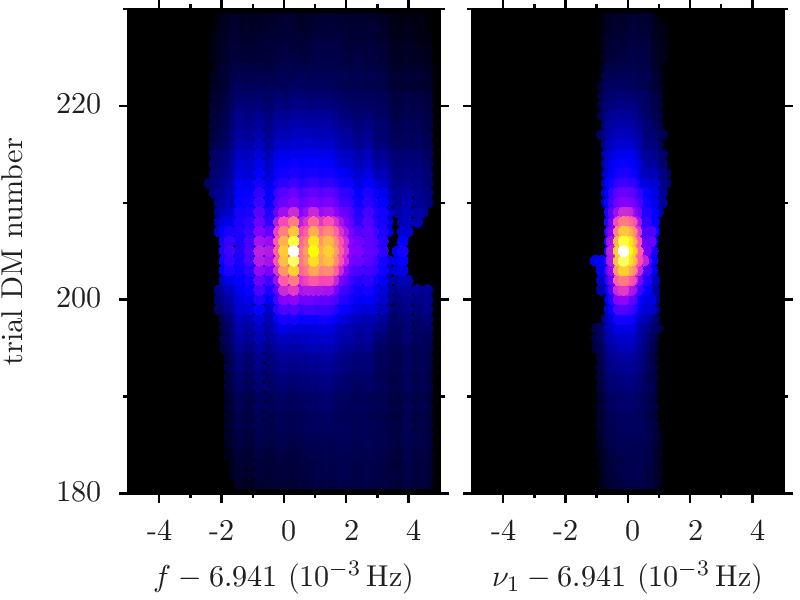
Figure 9.— The use of new plotting coordinates reduces the parameter spread, grouping physically related candidate signals closer together. (Left) Significance $\mathcal{S}$ as a function of spin frequency $f$ and dispersion measure DM for the detection of the relativistic pulsar J1906$+$0746 in the PMPS data. (Right) Significance $\mathcal{S}$ as a function of the spin frequency $\nu_{1}$ at the detector, and DM for the same data set. Note the significant reduction of data point spread by about a factor four. This reduction is not due to a scaling but due to resolving correlations between the physical parameters, as discussed below Eq. (A1).

Effectively, $\nu_{1}$ defines a the signal frequency at the detector at the beginning of the observation. The second coefficient, $\nu_{2}$, is proportional to the change of that frequency. This can be seen from taking the partial time derivative $1/(2\pi)\partial/\partial t$ of Eq. (A1)

$$f(t)=\sum_{j=1}^{\infty}j\nu_{j}t^{j-1}=\nu_{1}+2\nu_{2}t+\cdots$$ (A3)

References

- Aasi et al. (2012) Aasi, J., Abadie, J., Abbott, B. P., et al. 2012, ArXiv e-prints, arXiv:1207.7176 [gr-qc]
- Abbott et al. (2009a) Abbott, B., Abbott, R., Adhikari, R., et al. 2009a, Phys. Rev. D, 79, 022001
- Abbott et al. (2007) Abbott, B. P., et al. 2007, Phys. Rev. D, 76, 082001
- Abbott et al. (2009b) Abbott, B. P., Abbott, R., Adhikari, R., et al. 2009b, Phys. Rev. D, 80, 042003
- Allen et al. (2013) Allen, B., Knispel, B., Cordes, J. M., et al. 2013, ArXiv e-prints, arXiv:1303.0028 [astro-ph.IM]
- Anderson et al. (2006) Anderson, D. P., Christensen, C., & Allen, B. 2006, in Proceedings of the 2006 ACM/IEEE conference on Supercomputing, SC ’06 (New York, NY, USA: ACM)
- Aulbert & Fehrmann (2009) Aulbert, C., & Fehrmann, H. 2009, Max-Planck-Gesellschaft Jahrbuch 2009
- Bates et al. (2012) Bates, S. D., Bailes, M., Barsdell, B. R., et al. 2012, MNRAS, 427, 1052
- Belczynski et al. (2008) Belczynski, K., Kalogera, V., Rasio, F. A., et al. 2008, ApJS, 174, 223
- Bhat et al. (2004) Bhat, N. D. R., Cordes, J. M., Camilo, F., Nice, D. J., & Lorimer, D. R. 2004, ApJ, 605, 759
- Brady & Creighton (2000) Brady, P. R., & Creighton, T. 2000, Phys. Rev. D, 61, 082001
- Breton et al. (2007) Breton, R. P., Roberts, M. S. E., Ransom, S. M., et al. 2007, ApJ, 661, 1073
- Camilo et al. (2001) Camilo, F., Lyne, A. G., Manchester, R. N., et al. 2001, ApJ, 548, L187
- Champion et al. (2008) Champion, D. J., Ransom, S. M., Lazarus, P., et al. 2008, Science, 320, 1309
- Corbet (1984) Corbet, R. H. D. 1984, A&A, 141, 91
- Cordes et al. (2004) Cordes, J. M., Kramer, M., Lazio, T. J. W., et al. 2004, New Astronomy Reviews, 48, 1413
- Cordes & Lazio (2002) Cordes, J. M., & Lazio, T. J. W. 2002, ArXiv Astrophysics e-prints, arXiv:astro-ph/0207156
- Cordes & McLaughlin (2003) Cordes, J. M., & McLaughlin, M. A. 2003, ApJ, 596, 1142
- Cordes et al. (2006) Cordes, J. M., Freire, P. C. C., Lorimer, D. R., et al. 2006, ApJ, 637, 446
- Crawford et al. (2012) Crawford, F., Stovall, K., Lyne, A. G., et al. 2012, ApJ, 757, 90
- Damour & Schaefer (1991) Damour, T., & Schaefer, G. 1991, Physical Review Letters, 66, 2549
- Eatough et al. (2013) Eatough, R., Kramer, M., Lyne, A., & Keith, M. 2013, MNRAS, arXiv:1301.6346
- Eatough (2009) Eatough, R. P. 2009, PhD thesis, The University of Manchester
- Faucher-Giguère & Kaspi (2006) Faucher-Giguère, C.-A., & Kaspi, V. M. 2006, ApJ, 643, 332
- Faulkner et al. (2004) Faulkner, A. J., Stairs, I. H., Kramer, M., et al. 2004, MNRAS, 355, 147
- Faulkner et al. (2005) Faulkner, A. J., Kramer, M., Lyne, A. G., et al. 2005, ApJ, 618, L119
- Freire (2005) Freire, P. C. C. 2005, in Astronomical Society of the Pacific Conference Series, Vol. 328, Binary Radio Pulsars, ed. F. A. Rasio & I. H. Stairs, 405
- Freire et al. (2012a) Freire, P. C. C., Kramer, M., & Wex, N. 2012a, Classical and Quantum Gravity, 29, 184007
- Freire et al. (2012b) Freire, P. C. C., Wex, N., Esposito-Farèse, G., et al. 2012b, MNRAS, 423, 3328
- Frigo & Johnson. (2010) Frigo, M., & Johnson., S. G. 2010
- Fruchter et al. (1988) Fruchter, A. S., Stinebring, D. R., & Taylor, J. H. 1988, Nature, 333, 237
- Galassi (2009) Galassi, M. e. a. 2009, GNU Scientific Library Reference Manual - Third Edition
- Harry et al. (2009) Harry, I. W., Allen, B., & Sathyaprakash, B. S. 2009, Phys. Rev. D, 80, 104014
- Hobbs et al. (2004) Hobbs, G., Faulkner, A., Stairs, I. H., et al. 2004, MNRAS, 352, 1439
- Johnston & Kulkarni (1991) Johnston, H. M., & Kulkarni, S. R. 1991, ApJ, 368, 504
- Jouteux et al. (2002) Jouteux, S., Ramachandran, R., Stappers, B. W., Jonker, P. G., & van der Klis, M. 2002, A&A, 384, 532
- Keane (2010) Keane, E. F. 2010, PhD thesis, University of Manchester
- Keane (2012) Keane, E. F. 2012, in Proceedings of IAUS 291 ”Neutron Stars and Pulsars: Challenges and Opportunities after 80 years”
- Keane et al. (2010) Keane, E. F., Ludovici, D. A., Eatough, R. P., et al. 2010, MNRAS, 401, 1057
- Keith et al. (2009) Keith, M. J., Eatough, R. P., Lyne, A. G., et al. 2009, MNRAS, 395, 837
- Keith et al. (2010) Keith, M. J., Jameson, A., van Straten, W., et al. 2010, MNRAS, 409, 619
- Kerr et al. (2012) Kerr, M., Camilo, F., Johnson, T. J., et al. 2012, ApJ, 748, L2
- Kim et al. (2003) Kim, C., Kalogera, V., & Lorimer, D. R. 2003, ApJ, 584, 985
- Knispel (2011) Knispel, B. 2011, PhD thesis, Leibniz Universität Hannover
- Knispel et al. (2010) Knispel, B., Allen, B., Cordes, J. M., et al. 2010, Science, 329, 1305
- Knispel et al. (2011) Knispel, B., Lazarus, P., Allen, B., et al. 2011, ApJ, 732, L1
- Kramer et al. (2004) Kramer, M., Backer, D. C., Cordes, J. M., et al. 2004, New Astronomy Reviews, 48, 993
- Kramer et al. (2006a) Kramer, M., Lyne, A. G., O’Brien, J. T., Jordan, C. A., & Lorimer, D. R. 2006a, Science, 312, 549
- Kramer et al. (2003) Kramer, M., Bell, J. F., Manchester, R. N., et al. 2003, MNRAS, 342, 1299
- Kramer et al. (2006b) Kramer, M., Stairs, I. H., Manchester, R. N., et al. 2006b, Science, 314, 97
- Lorimer & Kramer (2005) Lorimer, D., & Kramer, M. 2005, Handbook of Pulsar Astronomy (Cambridge University Press)
- Lorimer (2012) Lorimer, D. R. 2012, in Proceedings of IAUS 291 ”Neutron Stars and Pulsars: Challenges and Opportunities after 80 years”
- Lorimer et al. (2012) Lorimer, D. R., Lyne, A. G., McLaughlin, M. A., et al. 2012, ApJ, 758, 141
- Lorimer et al. (2006) Lorimer, D. R., Faulkner, A. J., Lyne, A. G., et al. 2006, MNRAS, 372, 777
- Manchester et al. (2005) Manchester, R. N., Hobbs, G. B., Teoh, A., & Hobbs, M. 2005, VizieR Online Data Catalog, 7245, 0
- Manchester et al. (2001) Manchester, R. N., Lyne, A. G., Camilo, F., et al. 2001, MNRAS, 328, 17
- Messenger et al. (2009) Messenger, C., Prix, R., & Papa, M. A. 2009, Phys. Rev. D, 79, 104017
- Mickaliger et al. (2012) Mickaliger, M. B., Lorimer, D. R., Boyles, J., et al. 2012, ApJ, 759, 127
- Morris et al. (2002) Morris, D. J., Hobbs, G., Lyne, A. G., et al. 2002, MNRAS, 335, 275
- Owen (1996) Owen, B. J. 1996, Phys. Rev. D, 53, 6749
- Owen & Sathyaprakash (1999) Owen, B. J., & Sathyaprakash, B. S. 1999, Phys. Rev. D, 60, 022002
- Phinney (1992) Phinney, E. S. 1992, Royal Society of London Philosophical Transactions Series A, 341, 39
- Pletsch (2008) Pletsch, H. J. 2008, PRD, 78, 102005
- Ransom et al. (2003) Ransom, S. M., Cordes, J. M., & Eikenberry, S. S. 2003, ApJ, 589, 911
- Ransom et al. (2002) Ransom, S. M., Eikenberry, S. S., & Middleditch, J. 2002, AJ, 124, 1788
- Shao & Wex (2012) Shao, L., & Wex, N. 2012, Classical and Quantum Gravity, 29, 215018
- Stairs (2004) Stairs, I. H. 2004, Science, 304, 547
- Staveley-Smith et al. (1996) Staveley-Smith, L., Wilson, W. E., Bird, T. S., et al. 1996, Publications Astronomical Society of Australia, 13, 243
- Tauris (2011) Tauris, T. M. 2011, in Astronomical Society of the Pacific Conference Series, Vol. 447, Evolution of Compact Binaries, ed. L. Schmidtobreick, M. R. Schreiber, & C. Tappert, 285
- Tauris & Savonije (1999) Tauris, T. M., & Savonije, G. J. 1999, A&A, 350, 928
- Taylor & Weisberg (1989) Taylor, J. H., & Weisberg, J. M. 1989, ApJ, 345, 434
- Wood et al. (1991) Wood, K. S., Norris, J. P., Hertz, P., et al. 1991, ApJ, 379, 295