Weak-Value Amplification of light deflection by a dark atomic ensemble

Abstract

We study the coherent propagation of light whose dynamics is governed by the effective Schrödinger equation derived in a magneto-optically-manipulated atomic ensemble with a four-level tripod configuration for electromagnetically induced transparency (EIT). The small transverse deflection of an optical beam, which is ultra-sensitive to the EIT effect, could be drastically amplified via a weak measurement with an appropriate preselection and postselection of the polarization state. The physical mechanism is explained as the effect of wavepacket reshaping, which results in an enlarged group velocity in the transverse direction.

I Introduction

The weak measurement proposed by Aharonov, Albert and Vaidamn (AAV) WVPRL60 ; qparadox is usually referred to an amplification effect for weak signals rather than a conventional quantum measurement that collapses a coherent superposition of quantum states VonNm . In the original Gedanken experiment WVPRL60 , a seemingly surprising effect was proposed as it is possible to “measure” an appropriate preselected state of the spin-$1/2$ particle to obtain the average spin beyond the bound $\left[-0.5,0.5\right]$ of the smallest and largest eigenvalues. Such average spin (called weak value) does not exactly reflect the reality of a single spin, and is only the ensemble average of the measured data over a postselected subset. In this sense, the weak measurement implies some amplification of the resulting signal in the apparatus carrying on the pre- and post- selections WVpr12 . Several groups have studied such weak value amplification (WVA) effect in various physical systems, such as quantum optical phoPRL91 ; phoPRL05 ; SagPRL09 ; GCGuoA06 and condensed matter systems WilRL08 ; RomPRL08 . Note that WVA has been utilized as a quantum-coherent manipulation to engineer various interesting quantum effects, such as superluminal effects in birefringent optic fiber lumPRL04 , ultra-sensitive beam deflection SagPRL09 and optical spin-Hall effects Bliokh06 ; OSHE08 ; OSHE08F ; OSHE08n ; Gorod12 .

In this paper, we study the weak-value problem of spin-$1/2$ with polarized light beams propagating in a dispersive medium, a four-level atomic ensemble controlled by external fields. The motion of the light-wave envelope in such a coherent medium is described by an effective Schrödinger equation resembling the precession of a spin-$1/2$ in an inhomogeneous magnetic field DLZhou07 ; ZhouA08 ; ZhangA09 ; GuoA08 . However, because the effective magnetic field is very weak due to the inhomogeneity of the coupling transitions, the deflection of the light beam is usually difficult to observe even for EIT with two-photon resonance. For example, in the experiment by Karpa and Weitz Karpa06 , the angle of deflection is only about $2\times 10^{-5}$ rad when the light passes through a gas cell $5$cm long.

Since our concern here is only the deflection of the optical beam rather than the enhancement of the beam split, and the two beam’s split may be deflected in the same direction, we consider weak measurements to achieve this goal. According to our previous series of studies DLZhou07 ; ZhouA08 ; GuoA08 ; ZhangA09 , the motion of the transverse wavepacket is described by a Schrödinger-like equation, similar to that for the spin-$1/2$ in a transversely-inhomogeneous magnetic field in the Stern-Gerlach experiment GuoA08 . Thus, the peak of the optical beam will split into two, according to the initial polarization, under the influence of the transverse magnetic field gradient. When making a postselection on the final polarized state, the projection on this chosen polarization state mixes the two local wave packets in the transverse split. If such a weak measurement does not deform too much the shape of wavepacket, the transverse distance of the reshaped wavepacket from the center of the beam may be very large compared to that for any peaks in the optical Stern-Gerlach experiment. We carry out the relevant calculations in detail by making use of the effective field approach Lukin ; Lukin1 .

This paper is organized as follows. In Sec. II, we present a theoretical model for a four-level atomic ensemble with tripod configuration in the presence of nonuniform external fields, and derive the system of equations for the dynamics of the signal field in the atomic linear response with respect to the probe field. In Sec. III, we present the optical Stern-Gerlach effect of the probe beam in momentum space, which is induced by the interaction between the dispersive atomic medium and probe field used for EIT. In Sec. IV, we theoretically study the transverse deflection of the probe field via weak measurements, which can amplify signals by appropriate preselected and postselected states of the system. We conclude our paper in the final section.

II model setup

Consider an ensemble of $N$ identical and noninteracting atoms confined in a rectangular gas-cell, characterized by the ground-state Zeeman sublevels $\left|\pm\right\rangle$, one intermediate state $\left|s\right\rangle$, and an excited state $\left|e\right\rangle$, as shown in Fig. 1. The levels are coupled by two optical fields: a control laser field with frequency $\nu_{c}$ and wave-number $k_{c}$, and a probe laser field with frequency $\nu$ and wave-number $k$. The control field is assumed to be homogeneous and strong enough for propagation effects to be neglected, which was tuned to the $\left|s\right\rangle\rightarrow\left|e\right\rangle$ transition. The coupling strength is characterized by the Rabi frequency $\Omega$. The probe laser field is linearly-polarized and propagating along the $z$-axis. Its linear polarization is a superposition of left- and right-handed circular polarization, labelled by $\sigma_{\pm}$. We denote the $\sigma_{j}$-polarized component as $\tilde{E}_{j}\left(\mathbf{r},t\right),j=\pm$, which drives the transitions $\left|\pm\right\rangle\leftrightarrow\left|e\right\rangle$, respectively.

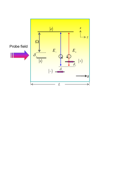
Figure 1: (Color online) Schematic diagram of an atomic ensemble with a four-level tripod configuration in a gas cell of length $L$, manipulated by two optical and one magnetic fields. The magnetic field $B$ is applied along the $z$-direction with a gradient along the $x$-direction.

The atomic gas cell can be divided into many smaller cells. We assume that each smaller cell contains a large number of atoms and the inhomogeneous external field is sufficiently homogeneous for each smaller cell DLZhou07 . In this case, the atomic medium can be treated in a continuous way by the following approach. First, describe the medium excitation by introducing the collective atomic operators $\tilde{\Xi}_{\mu\nu}\left(\mathbf{r}\right)=(1/N_{\mathbf{r}})\sum_{j=1}^{N_{\mathbf{r}}}\tilde{\Xi}_{\mu\nu}^{j}$, averaged over a small but macroscopic volume containing many atoms $N_{\mathbf{r}}=(N/V)dV\gg 1$ around position $\mathbf{r}$. Here, $\tilde{\Xi}_{\mu\nu}^{j}\left(\mathbf{r}\right)=\left|\mu\right\rangle_{j}\langle\nu|$. Afterwards replace the sum over the total number $N$ of atoms by $\frac{N}{V}\int d^{3}r$, where $V$ is the volume of the medium Lukin ; Lukin1 . Neglecting the kinetic energy of the atoms, the Hamiltonian of the atomic part is given by

$$H^{(A)}=\frac{N}{V}\sum_{i}\int d^{3}r\left(\omega_{i}+\mu_{i}B\right)\tilde{\Xi}_{ii}$$ (1)

where $\omega_{i}$ $(i=\pm,s,e)$ are the bare atomic energies, and $\omega_{\pm}=\omega_{0}$ (which corresponds to degenerate levels when $B=0$). The magnetic field $B$ along the $z$-axis shifts the energy levels by the amount $\mu_{i}B\left(\mathbf{r}\right)$, where the magnetic moments, $\mu_{i}=m_{F}^{i}g_{F}^{i}\mu_{B}$, are defined by the Bohr magneton $\mu_{B}$, the gyromagnetic factor $g_{F}^{i}$, and the magnetic quantum number $m_{F}^{i}$ of the corresponding state $\left|i\right\rangle$. Under the electric-dipole approximation and the rotating-wave approximation, the light-matter interaction Hamiltonian becomes Lukin ; Lukin1

$$H^{(I)} = \frac{N}{V}\int\Omega\;e^{i\left(\mathbf{k}_{c}\cdot\mathbf{r}-\nu_{c}t\right)}\;\tilde{\Xi}_{es}\;d^{3}r+h.c.$$

$$+\frac{N}{V}\sum_{j=\pm}d_{ej}\int\tilde{E}_{j}^{\left(+\right)}\;\tilde{\Xi}_{ej}\;d^{3}r+h.c.,$$

with $d_{e-}(d_{e+})$ denoting the matrix element of the dipole momentum operator projected on the direction of the electric field.

The slow-varying variables $E_{j}(\mathbf{r},t)$ for the probe field and the collective atomic transition operators $\Theta_{\alpha\beta}$ can be defined as

$$\tilde{E}_{j}^{+}(\mathbf{r},t) = \sqrt{\frac{\nu}{2\varepsilon_{0}V}}E_{j}(\mathbf{r},t)e^{i(kz-\nu t)},\;(j=\pm)\text{,}$$ (3a)

$$\tilde{\Xi}_{ej} = \Theta_{ej}\exp(-ikz)\text{,}$$ (3b)

$$\tilde{\Xi}_{es} = \Theta_{es}\exp(-i\mathbf{k}_{c}\cdot\mathbf{r})\text{.}$$ (3c)

In a rotating reference frame, the dynamics of this system is described by

$$H_{{\rm rot}} = \frac{N}{V}\int d^{3}r\left(\delta_{-}\Theta_{--}+\delta_{+}\Theta_{++}+\delta_{c}\Theta_{ss}\right)$$

$$+\frac{N}{V}\int d^{3}r\left(\Omega\Theta_{es}+\sum_{j=\pm}g_{j}E_{j}\Theta_{ej}\right)+h.c.$$

with $\delta_{i}$ $(i=\pm,c)$ the detunings of the probe and control fields from the corresponding atomic transitions given as

$$\delta_{c} =\omega_{s}-\omega_{e}+\nu_{c}+\left(\mu_{s}-\mu_{e}\right)B,$$

$$\delta_{\pm} =\omega_{\pm}-\omega_{e}+\nu+\left(\mu_{\pm}-\mu_{e}\right)B,$$

and the coupling strength as

$$g_{j}=d_{ej}\sqrt{\frac{\nu}{2\varepsilon_{0}V}}.$$ (5)

The Hamiltonian in Eq. (II) generates the Heisenberg equations of the slowly-varying variables $\Theta_{\mu\nu}$. The Langevin equations are obtained to describe the dynamics of the medium by introducing the coherence relaxation rate $\gamma$ between the ground state $|\pm\rangle$ and the intermediate state $\left|s\right\rangle$, as well as the decay rate $\Gamma$ of the excited state. The low intensity approximation Lukin ; Lukin1 ; SunPRL01 , on one hand, allows us to neglect Langevin noise operators since the number of photons contained in the probe laser beams is much smaller than the number of atoms in the sample, so the operators become c-numbers. On the other hand, it allows us to regard the interaction between the matter and the probe field as a weak disturbance, since the intensity of the probe laser beams is much weaker than that of the control laser field. The perturbation approach Lukin ; Lukin1 ; Petrosyan can be applied in terms of a power series in $gE_{j}$:

$$\Theta_{\alpha\beta}=\Theta_{\alpha\beta}^{(0)}+\varepsilon\Theta_{\alpha\beta}^{(1)}+\cdots$$ (6)

where $\varepsilon$ is a parameter that ranges continuously between zero and one. When $\varepsilon=0$, the probe field is absent. For all atoms initially in level $|\pm\rangle$ without polarization (i.e., atom $i$ in a mixed state $\rho_{i}=\Sigma_{j=\pm}|j\rangle\langle j|/2$), we obtain

$$\Theta_{--}^{(0)}=\Theta_{++}^{(0)}=\frac{1}{2}$$ (7)

while all others terms vanish. Here, we retain only terms up to the first-order in $\varepsilon$, since the linear optical response theory can sufficiently reflect the main physical features. The dispersion and absorption are determined by $\Theta_{je}^{(1)}$, which is obtained as

$$\Theta_{je}^{\left[1\right]}=-\frac{\Delta_{j}\,g_{j}\,E_{j}}{2\Omega\,\Omega^{\ast}},\,\,(j=\pm)$$ (8)

in the steady-state solutions GuoA08 ; ZhangA09 ; Petrosyan , where pure dephasing processes and decay among the lower states are neglected ($\gamma=0$) to highlight the main physics, and a sufficiently strong driving field is assumed to satisfy $\left|\Omega\right|^{2}\gg\Gamma\gamma,\Delta_{j}^{2}$. We note the assumption on the strong driving field implies that $\left|\Omega\right|\gg\left|\left(\mu_{+}-\mu_{-}\right)B\right|$. The Raman detuning is defined as

$$\Delta_{j}=\delta_{j}-\delta_{c},$$ (9)

which leads to a spatially-varying refractive index profile in the gas cell DLZhou07 due to the small transverse magnetic field gradient.

Using the slowly-varying-envelope approximation, the paraxial wave equation in the linear optical response theory Lukin ; Lukin1 ; Petrosyan

$$\left(i\partial_{t}+ic\partial_{z}\right)E_{j}=-Ng_{j}^{\ast}\Theta_{je}^{(1)},$$ (10)

becomes an effective Schrödinger equation

$$i\partial_{t}E_{j}=H_{j}E_{j},$$ (11)

by substituting Eq. (8) into (10), where the effective Hamiltonian is

$$H_{j}=cp_{z}+\frac{N\left|g_{j}\right|^{2}}{2\left|\Omega\right|^{2}}\Delta_{j}.$$ (12)

Here $c$ is the velocity of light in vacuum and $p_{z}=-i\partial_{z}$. Notice that the $\sigma_{\pm}$-polarization accompany the component $E_{\pm}$. Writing the $\sigma_{\pm}$-polarization states as column vectors resembling the spin-$1/2$

$$\left|\sigma_{+}\right\rangle = \left[\begin{array}[]{cc}1&0\end{array}\right]^{T},$$ (13b)

$$\left|\sigma_{-}\right\rangle = \left[\begin{array}[]{cc}0&1\end{array}\right]^{T},$$ (13d)

where the superscript $$T E_{\pm} \Phi=\left[E_{+},E_{-}\right]^{T}$$ means transpose, we can group the two components into a column vector defined as the “spinor state” . The dynamical equation of the probe laser field reads

$$i\partial_{t}\Phi=\left[\begin{array}[]{cc}H_{+}&0\\ 0&H_{-}\end{array}\right]\Phi=H_{{\rm eff}}\Phi,$$ (14)

which allows us to write the state of the probe laser field at any arbitrary time as

$$\left|\Phi\left(t\right)\right\rangle=\sum_{j=\pm}c_{j}\left|E_{j}\left(t\right)\right\rangle\left|\sigma_{j}\right\rangle.$$ (15)

Here, the states $\left|E_{j}\right\rangle$ describe the state of the spatial degrees of freedom, with $E_{j}\left(\mathbf{r},t\right)$ referred to as the corresponding spatial representation.

Hereafter, to investigate the beam deflection amplification of light beam, propagating in the dispersive atomic ensemble, we use a signal enhancement technique known from weak measurements Aharonov90 . Along with the standard weak measurement terminology, the transverse position degree of freedom of the probe beam is referred to as the meter and its intrinsic polarization degree of freedom is referred to as the measured system.

III optical Stern-Gerlach effect

We now investigate the evolution of the probe wave packet. The polarization vector of the probe field lies in the plane perpendicular to its travelling direction (i.e., the $z$-direction). It is initially prepared in a superposition state

$$\left|i\right\rangle=\cos\frac{\alpha}{2}\left|H\right\rangle+\sin\frac{\alpha}{2}\left|V\right\rangle,$$ (16)

of the horizontal polarization, $|H\rangle=\left(\left|\sigma_{+}\right\rangle+\left|\sigma_{-}\right\rangle\right)/\sqrt{2}$, and vertical polarization, $|V\rangle=-i\left(\left|\sigma_{+}\right\rangle-\left|\sigma_{-}\right\rangle\right)/\sqrt{2}$, where $\alpha$ is the polarization angle of the probe light beam. For weak measurement, this angle is very small, which means that the probe field is initially almost in the horizontal polarization state. The role of $\alpha$ in the transverse beam deflection amplification via weak measurements will be further discussed in the next section.

The two components of the probe field travel collinearly before reaching the medium, which implies that initially $\left|E_{j}\left(t_{0}\right)\right\rangle=\left|E_{0}\left(0\right)\right\rangle$, where the initial time $t_{0}=0$. After the probe field enters the medium, the atomic ensemble induces the time evolution operator $U(t)=e^{-iH_{{\rm eff}}t}$ on the meter state according to their polarized state. Then the state at an arbitrary time becomes an entangled state

$$\left|\Phi\left(t\right)\right\rangle=\frac{1}{\sqrt{2}}\left(e^{-i\alpha/2}|\sigma_{+}\rangle|E_{+}(t)\rangle+e^{i\alpha/2}|\sigma_{-}\rangle|E_{-}(t)\rangle\right),$$ (17)

where the meter state is described by

$$\left|E_{j}(t)\right\rangle=e^{-iH_{j}t}\left|E_{0}(0)\right\rangle.$$ (18)

We will show that $E_{\pm}\left(\mathbf{r},t\right)$ in Eq. $\left(\ref{Sec3-02}\right)$ implies a wavepacket split in momentum space according to polarizations. After a measurement on the postselected state $|V\rangle$, the meter is reshaped as

$$\left|\Phi_{f}^{m}\left(t\right)\right\rangle=\frac{i}{2}\left(e^{-i\frac{\alpha}{2}}\left|E_{+}(t)\right\rangle-e^{i\frac{\alpha}{2}}\left|E_{-}(t)\right\rangle\right).$$ (19)

Obviously, the superposition of the two wavepackets $E_{\pm}\left(\mathbf{r},t\right)$ can produce an interference pattern in the coordinate space.

Figure 2: (Color online) Optical Stern-Gerlach effect in momentum space with the transverse distribution $\left|E_{j}\left(k_{x},t_{f}\right)\right|^{2}$ as a function of wave number $k_{x}=p_{x}/\hbar$, right after the light leaves the EIT medium. Here, $k_{x}$ is in units of reciprocal meters.

Now we assume that the magnetic field $B$ applied in the $z$-direction has a linear gradient along the $x$-direction with the expression

$$B=B_{0}+B_{1}x.$$ (20)

Here, our treatment is confined to only one transverse dimension, say the $x$-direction. The effective Hamiltonian in Eq.(12) reads

$$H_{j}=cp_{z}+b_{0j}+b_{1j}x,$$ (21)

where the parameters

$$b_{0j} = \frac{N\left|g_{j}\right|^{2}}{2\left|\Omega\right|^{2}}\left[\omega_{j}+\nu-\omega_{s}-\nu_{c}+\left(\mu_{j}-\mu_{s}\right)B_{0}\right],$$ (22a)

$$b_{1j} = \frac{N\left|g_{j}\right|^{2}}{2\left|\Omega\right|^{2}}\left(\mu_{j}-\mu_{s}\right)B_{1},$$ (22b)

can be adjusted by the control laser field and the magnetic field as well as the energy levels. For an initial state with a two-dimensional Gaussian amplitude profile

$$E_{j}\left(r,0\right)=\frac{1}{\sqrt{2\pi a^{2}}}\exp\left(-\frac{z^{2}+x^{2}}{4a^{2}}\right),$$ (23)

the EIT medium introduces different phase shifts on the meter wavepacket according to the right-handed or left-handed circularly-polarized state, and a displacement $ct$ along the $z$-direction

$$E_{j}\left(r,t\right)=\frac{e^{-itb_{0j}}}{\sqrt{2\pi a^{2}}}\exp\left[-\frac{(z-ct)^{2}+x^{2}}{4a^{2}}-itb_{1j}x\right].$$ (24)

Since $\left[H_{j},x\right]=0$, the center of $E_{j}\left(\mathbf{r},t\right)$ does not change with time, $\left\langle x_{j}\right\rangle=0$, which implies no spatial split of the meter wavepacket. A Fourier transformation on Eq.( 24)

$$E_{j}\left(k,t\right)= 2\sqrt{2a^{2}\pi}\exp(-ib_{0j}t-a^{2}k_{z}^{2}-ick_{z}t)$$

$$\times\exp[-a^{2}\left(k_{x}+b_{1j}t\right)^{2}]$$

shows that each meter’s wavepacket keeps the longitudinal momentum unchanged and acquires a transverse momentum with magnitude $b_{1j}t$, which is a linear function of time. Therefore, two wavepackets of the probe field have the same centroid, but achieve different momenta in the $x$-direction inside the EIT medium. To illustrate the split of the probe beam in momentum space, we assume that the probe beam with an initial width $a=2$ mm is tuned to the rubidium (⁸⁷Rb) D1-line $5^{{}^{2}}S_{{}_{1/2}}\leftrightarrow 5^{{}^{2}}P_{{}_{1/2}}$, that the ground states $\left|\pm\right\rangle$ correspond to the magnetic sublevels (with $m_{F}=1$ and $-1$) of the $F=1$ hyperfine ground state, and that $\left|s\right\rangle$ represents the hyperfine ground state $\left|F=2,m_{F}=1\right\rangle$. In this case, the phase shift on the $\sigma_{-}$-component vanishes due to $\mu_{s}=\mu_{-}=4.64\times 10^{-24}\,{\rm JT}^{-1}$. Hence, there is no shift of the momentum on the $\sigma_{-}$-component. The magnetic field gradient $B_{1}=910\,\mu{\rm Gmm}^{-1}$ and the magnetic moments $\mu_{+}=-\mu_{s}$ subject the wavepacket of the $\sigma_{+}$-component to a linear potential in the transverse direction. In Fig. 2, we show such an optical Stern-Gerlach effect in momentum space by plotting the transverse distribution $\left|E_{j}\left(k_{x},t_{f}\right)\right|^{2}$ as a function of the wavenumber $k_{x}=p_{x}/\hbar$ using the typical group velocities of a few thousand metres per second KarpaPRL at a fixed time $t_{f},$ where $t_{f}=L/c$ denotes the interaction time with $L=50$ mm as the cell length. Obviously, the transverse displacement is smaller than the uncertainty of the width of two wavepackets of the meter.

However, postselecting the system on a desired polarized state $\left|V\right\rangle$ leads to a coherent superposition of two transverse wavepackets. The interference of the two meter’s wavepackets displace the centroid of the wave packet in coordinate space by

$$\left\langle x\right\rangle=\frac{\sin\left(b_{0}t+\alpha\right)a^{2}b_{1}tf_{t}}{1-f_{t}\cos\left(b_{0}t+\alpha\right)},$$ (26)

where we have introduced $b_{0}=b_{0+}-b_{0-}$, $b_{1}=b_{1+}-b_{1-}$ and $f_{t}\equiv\exp\left(-a^{2}b_{1}^{2}t^{2}/2\right)$. We also note that when the optical beam is deflected by the EIT medium, the wave packet will spread in the transverse direction. This spread will blur the observation of deflection. To examine this, we calculate the transverse fluctuation

$$\left\langle\Delta x^{2}\right\rangle=a^{2}\frac{1+\left(a^{2}b_{1}^{2}t^{2}-2\right)f_{t}\cos\alpha+\left(\cos^{2}\alpha-a^{2}b_{1}^{2}t^{2}\right)f_{t}^{2}}{\left(1-f_{t}\cos\alpha\right)^{2}}$$

with $b_{0}=0$. Usually, only if $\langle\triangle x^{2}\rangle<\langle x\rangle^{2}$, we can clearly observe such deflection. Otherwise, i.e., $\langle\triangle x^{2}\rangle>\langle x\rangle^{2}$, the deflection will be blured by the transverse spreading of wavepackets. In this case, a weak-measurement technique is necessary to observe the extremely small deflection of the light beam.

IV weak value and deflection of the optical beam

In the previous section, we have shown that the projection measurement on the initial polarization described by the state $\left|i\right\rangle$ in Eq. (16), could induce the transverse displacement of the optical beam after light passes through an EIT medium. Now, we will consider the maximization of this transverse displacement, with the weak measurement proposed by Aharanov et al. WVPRL60 .

A weak measurement describes a situation where a system is so weakly coupled to a measuring device that the uncertainty in the measurement is larger than all the separations among the eigenvalues of the observable. Therefore, no information is given since the eigenvalues are not fully resolved. Three steps are necessary for weak measurements: 1) quantum state preparation (preselection); 2) a weak perturbation; 3) postselection on a final quantum state. The three essential ingredients of weak measurements were theoretically performed in the previous section.

First, we have initially prepared the state $\left|i\right\rangle$ of the system and a Guassian wave packet of the meter before the light is incident on the medium. Second, the polarization-dependent effective potential in Eq. (14) changes the polarized state as

$$\left|\phi\right\rangle=\frac{e^{-i\bar{\theta}_{x}t}}{\sqrt{2}}\left[\exp\left(i\frac{\alpha+b_{0}t}{2}\right)\exp\left(i\frac{b_{1}xt}{2}\right)\left|\sigma_{-}\right\rangle\right.$$ (27)

$$+\left.\exp\left(-i\frac{\alpha+b_{0}t}{2}\right)\exp\left(-i\frac{b_{1}xt}{2}\right)\left|\sigma_{+}\right\rangle\right]$$

with $\bar{\theta}_{x}=\left(\bar{b}_{0}+\bar{b}_{1}x\right)$, where $\bar{b}_{j}\equiv\left(b_{j+}+b_{j-}\right)/2$. The state $\left|\phi\right\rangle$ indicates that there is an interaction Hamiltonian between the system and the meter, $H_{{\rm int}}=\xi\sigma_{z}$ with $\xi=b_{1}x/2$, and a free evolution $\exp\left(-ib_{0}t\sigma_{z}/2\right)$ on the spin. Here, $\left|\sigma_{\pm}\right\rangle$ are the eigenstates of the Pauli operator $\sigma_{z}$ with eigenvalues $\pm 1$. A weak perturbation is guaranteed when the transverse displacement in momentum space is smaller than the width of the transverse distribution. In addition, the coupling strength $b_{1}$ could be adjusted by the control laser field and the magnetic field gradient.

Afterwards, the polarization state $|V\rangle$ is postselected. The information on the observable of the system is read out from the transverse spatial distribution which serves as the meter. However, the mean position in Eq. (26) is not the weak value. Weak measurements can provide the weak values defined by $\left\langle\sigma_{z}\right\rangle_{w}=\left\langle\psi_{{\rm fi}}\right|\hat{\sigma}_{z}\left|\psi_{{\rm in}}\right\rangle/\left\langle\psi_{{\rm fi}}\right.\left|\psi_{{\rm in}}\right\rangle$, where $\left|\psi_{{\rm in}}\right\rangle$ and $\left|\psi_{{\rm fi}}\right\rangle$ are the preselected and postselected states of the system, respectively. Here, they are given by

$$\left|\psi_{{\rm in}}\right\rangle\equiv \frac{e^{-i\bar{\theta}_{x}t}}{\sqrt{2}}\left[\exp\left(i\frac{\alpha+b_{0}t}{2}\right)\left|\sigma_{-}\right\rangle\right.$$ (28a)

$$\left.+\exp\left(-i\frac{\alpha+b_{0}t}{2}\right)\left|\sigma_{+}\right\rangle\right],$$

$$\left|\psi_{{\rm fi}}\right\rangle = \left|V\right\rangle.$$ (28b)

In our case, the observable is $\sigma_{z}$. Taking the free evolution of the spin into account, we obtain the weak value

$$\left\langle\sigma_{z}\right\rangle_{w}=\frac{\left\langle\psi_{{\rm fi}}\right|\sigma_{z}\left|\psi_{{\rm in}}\right\rangle}{\left\langle\psi_{{\rm fi}}\right.\left|\psi_{{\rm in}}\right\rangle}=i\cot\left(\frac{\alpha+b_{0}t}{2}\right)$$ (29)

From the definition of weak value, one can find that if the free evolution of the spin is not taken into account, the resulting weak value is $i\cot\left(\alpha/2\right)$, rather than the above result.

It is well known that the weak value is linked to the final read of the meter. To obtain the mean position, one should first expand $\left\langle\psi_{{\rm fi}}\right|\exp\left(-i\xi\sigma_{z}t\right)\left|\psi_{{\rm in}}\right\rangle$ until its first order in $b_{1}t$. Actually, this first-order expansion is valid in our system since we only consider the short-time behavior and the the external magnetic field gradient $B_{1}$ in the $x$-direction is very small; thus $b_{1}t\ll 1$ is satisfied. Then we write $\left\langle\psi_{{\rm fi}}\right|\sigma_{z}\left|\psi_{{\rm in}}\right\rangle$ in terms of the weak value $\left\langle\sigma_{z}\right\rangle_{w}$. Finally, we regroup it to an exponential function $\left\langle\psi_{{\rm fi}}\right.\left|\psi_{{\rm in}}\right\rangle\left(1-i\xi_{t}t\left\langle\sigma_{z}\right\rangle_{w}\right)\approx\left\langle\psi_{{\rm fi}}\right.\left|\psi_{{\rm in}}\right\rangle\exp\left(-i\xi_{t}t\left\langle\sigma_{z}\right\rangle_{w}\right)$, which yields

$$\left\langle x\right\rangle_{wv}=a^{2}b_{1}t\cot\left(\frac{\alpha+b_{0}t}{2}\right)$$ (30)

as the observed mean position of the meter.

Figure 3: (Color online) Transverse distribution of the probe field. The red solid curve corresponds to the Gaussian profile in Eq. (23). The black dashed curve depicts the norm square of the wavefunction in Eq. (32) with a weak measurement right after the light leaves the medium. The green dashed-dotted curve presents the normalized distribution of Eq. (19) at time $t_{f}=L/c$. Here, $x$ is in units of millimeters. $b_{0}t+\alpha=0.08$. Other parameters are the same as in Fig. 2.

It can be seen from Eq. (30) that the final read of the meter is proportional to the imaginary part of the weak value. To find the relation between the result in Eq. (26) and the weak value in Eq. (30), we rewrite Eq. (18) as

$$\left|E_{j}(t)\right\rangle=\exp[-i\left(cp_{z}+b_{0j}\right)t]\left(1-ib_{1j}xt\right)\left|E_{0}(0)\right\rangle$$ (31)

by retaining the linear term of the Taylor series expansion of $\exp\left(-ib_{1j}xt\right)$. After some algebra, we find that the mean position in Eq. (30) is a linear approximation of Eq. (26) with respect to the coupling between the system and the meter. After the postselection of the polarization degrees of freedom, the normalized wavepacket of the probe field in the transverse direction becomes

$$\Psi_{f}^{N}\left(x,t\right)=\frac{1}{\sqrt{2\pi a^{2}}}\exp\left(-\frac{x^{2}-x\left\langle x\right\rangle_{wv}+\left\langle x\right\rangle_{wv}^{2}}{4a^{2}}\right)\text{.}$$ (32)

In Fig. 3, we plot the transverse distribution of the incident wavepacket in Eq. (23) with a red solid curve, $|\Psi_{f}^{N}\left(x,t\right)|^{2}$ in Eq. (32) at time $t_{f}=L/c$ (black dashed curve), and the normalized norm square of Eq. (19) right after the probe field leaves the atomic medium (green dashed-dotted curve). Obviously, the weak measurement significantly enhances the deflection of the probe field.

Different from the mean value of a quantum-mechanical measurement, which must lie within the range of eigenvalues, weak values in Eq. (29) produce results much larger than any of the eigenvalues of an observable, particularly when one chooses the intial state $\left|\psi_{{\rm in}}\right\rangle$ with $\alpha=-b_{0}t_{f}$ (where $t_{f}$ is the total interaction time). By performing a weak measurement of the probe laser field that has passed through an EIT atomic medium, we are able to significantly magnify the transverse displacement of the probe field, which results in a large group velocity $d\left\langle x\right\rangle_{wv}/dt$ in the transverse direction. The deflection angle given in Ref. Karpa06 is defined as $\theta=c^{-1}d\left\langle x\right\rangle_{wv}/dt$. When $b_{0}=0$, the deflection angle is totally decided by the original polarization angle $\alpha$. And the magnitude of the deflection angle could be arbitrarily large as $\alpha$ approaches zero. Comparing to the angle of deflection $2\times 10^{-5}$ rad for the EIT condition Karpa06 , the weak measurement technique discussed here drastically amplifies the displacement of the probe field in the transverse direction.

V discussion

We have theoretically studied a magneto-optically-controlled atomic ensemble under the EIT condition to couple a property (the observable $\sigma_{z}$) of the polarization (the system) with the spatial degree of freedom (the meter). In the paraxial regime, the dynamics of the transverse distribution is governed by an impulsive measurement interaction Hamiltonian $H_{{\rm int}}=\xi\sigma_{z}$, which makes the displacements of the transverse spatial components polarization-dependent. An enhanced displacement in the meter distribution is achieved by an appropriate preselection and postselection of the polarization state. However, the choice of the preselected state is dependent on the accumulated phase during the free evolution of the system with the weak measurement taking place in between.

This work is supported by NSFC No. 11074071, NFRPC 2012CB922103, PCSIRT No. IRT0964, Hunan Provincial Natural Science Foundation of China (11JJ7001 and 12JJ1002). FN is partially supported by the ARO, JSPS-RFBR contract No. 12-02-92100, Grant-in-Aid for Scientific Research (S), MEXT Kakenhi on Quantum Cybernetics, and the JSPS via its FIRST program.

References

- (1) Y. Aharonov, D.Z. Albert, and L. Vaidman, Phys. Rev. Lett. 60, 1351 (1988).
- (2) Y. Aharonov, D. Rohrlich, Quantum Paradoxes- Quantum Theory for the Perplexed (WILEY-VCH Verlag GmbH & Co. KGaA).
- (3) J.V Neumann, Mathematical Foundations of Quantum Mechanics (Princeton University Press, Princeton 1955); German Version 1932.
- (4) A.G. Kofman, S. Ashhab, and F. Nori, Phys. Rep. 520, 43 (2012).
- (5) N.W.M. Ritchie, J.G. Story, and R.G. Hulet, Phys. Rev. Lett. 66, 1107 (1991).
- (6) G.J. Pryde, J.L. O’Brien, A.G. White, T.C. Ralph, and H.M. Wiseman, Phys. Rev. Lett. 94, 220405 (2005).
- (7) P.B. Dixon, D.J. Starling, A.N. Jordan, and J.C. Howell, Phys. Rev. Lett. 102, 173601 (2009).
- (8) Q. Wang, F.-W. Sun, Y.-S. Zhang, Jian-Li, Y.-F. Huang, G.-C. Guo, Phys. Rev. A 73, 023814 (2006).
- (9) N. S. Williams and A. N. Jordan, Phys. Rev. Lett. 100, 026804 (2008).
- (10) A. Romito, Y. Gefen, and Y.M. Blanter, Phys. Rev. Lett. 100, 056801 (2008).
- (11) N. Brunner, V. Scarani, M. Wegmüller, M. Legré and N. Gisin, Phys. Rev. Lett. 93, 203902 (2004).
- (12) K.Y. Bliokh and Y.P. Bliokh, Phys. Rev. Lett. 96, 073903 (2006).
- (13) O. Hosten and P. Kwiat, Science 319, 787 (2008).
- (14) F. Nori, Nature Photon. 2, 716 (2008).
- (15) K.Y. Bliokh, A. Niv, V. Kleiner, and E. Hasman, Nature Photon. 2, 748 (2008).
- (16) Y. Gorodetski, K. Y. Bliokh, B. Stein, et al., Phys. Rev. Lett. 109, 013901 (2012).
- (17) L. Karpa and M. Weitz, Nature Phys. 2, 332 (2006)
- (18) D. L. Zhou, L. Zhou, R. Q. Wang, S. Yi, and C. P. Sun, Phys. Rev. A 76, 055801 (2007).
- (19) L. Zhou, J. Lu, D. L. Zhou, and C. P. Sun, Phys. Rev. A 77, 023816 (2008);
- (20) H. R. Zhang, L. Zhou, and C. P. Sun, Phys. Rev. A 80, 013812 (2009).
- (21) Y. Guo, L. Zhou, L. M. Kuang, and C. P. Sun, Phys. Rev. A 78, 013833 (2008);
- (22) M. Fleischhauer and M. D. Lukin, Phys. Rev. Lett. 84, 5094 (2000).
- (23) M. Fleischhauer and M. D. Lukin, Phys. Rev. A 65, 022314 (2002).
- (24) C. P. Sun, Y. Li, and X. F. Liu, Phys. Rev. Lett. 91, 147903 (2003).
- (25) D. Petrosyan and Y. P. Malakyan, Phys. Rev. A 70, 023822 (2004).
- (26) L. Karpa, F. Vewinger, and M. Weitz, Phys. Rev. Lett. 101, 170406 (2008).
- (27) Y. Aharonov and L. Vaidman, Phys. Rev. A 41, 11 (1990).