A Primer on Stochastic Differential Geometry for Signal Processing

Abstract

This primer explains how continuous-time stochastic processes (precisely, Brownian motion and other Itô diffusions) can be defined and studied on manifolds. No knowledge is assumed of either differential geometry or continuous-time processes. The arguably dry approach is avoided of first introducing differential geometry and only then introducing stochastic processes; both areas are motivated and developed jointly.

I Introduction

The tools of calculus — differentiation, integration, Taylor series, the chain rule and so forth — have extensions to curved surfaces and more abstract manifolds, and a different set of extensions to stochastic processes. Stochastic differential geometry brings together these two extensions.

This primer was written from the perspective that, to be useful, it should give more than a big-picture view by drilling down to shed light on important concepts otherwise obfuscated in highly technical language elsewhere. Gaining intuition, and gaining the ability to calculate, while going hand in hand, are distinct from each other. As there is ample material catering for the latter [1, 2, 3, 4], the focus is on the former.

Brownian motion plays an important role in both theoretical and practical aspects of signal processing. Section II is devoted to understanding how Brownian motion can be defined on a Riemannian manifold. The standpoint is that it is infinitely more useful to know how to simulate Brownian motion than to learn that the generator of Brownian motion on a manifold is the Laplace-Beltrami operator.

Stochastic development is introduced early on, in Section II-B, because “rolling without slipping” is a simple yet striking visual aid for understanding curvature, the key feature making manifolds more complicated and more interesting than Euclidean space. Section III explains how stochastic development can be used to extend the concept of state-space models from Euclidean space to manifolds. This motivates the introduction of stochastic differential equations in Section IV. Since textbooks abound on stochastic differential equations in Euclidean space, only a handful of pertinent facts are presented. As explained in Section V, and despite appearances [5, 2, 6], going from stochastic differential equations in Euclidean space to stochastic differential equations on manifolds is relatively straightforward conceptually if not technically.

Section VI examines more closely the theory of stochastic integration. It explains (perhaps in a novel way) how randomness can make it easier for integrals to exist. It clarifies seemingly contradictory statements in the literature about pathwise integration. Finally, it emphasises that despite the internal complexities, stochastic integrals are constructed in the same basic way as other integrals and, from that perspective, are no more complicated than any other linear operator.

The second half of the paper, starting with Section VII, culminates in the generalisation of Gaussian random variables to compact Lie groups and the re-derivation of the formulae in [7] for estimating the parameters of these random variables. Particular attention is given to the special orthogonal groups consisting of orthogonal matrices having unit determinant, otherwise known as the rotation groups. Symmetry makes Lie groups particularly nice to work with.

Estimation theory on manifolds is touched on in Section XI, the message being that an understanding of how an estimator will be used is needed to avoid making ad hoc choices about how to assess the performance of an estimator, including what it means for an estimator to be unbiased.

The reason for introducing continuous-time processes rather than ostensibly simpler discrete-time processes is that the only linear structure on manifolds is at the infinitesimal scale of tangent spaces, allowing the theory of continuous-time processes to carry over naturally to manifolds. A strategy for working with discrete-time processes is treating them as sampled versions of continuous-time processes. In the same vein, Section IX uses Brownian motion to generalise Gaussian random variables to Lie groups.

There are numerous omissions from this primer. Even the Itô formula is not written down! Perhaps the most regrettable is not having the opportunity to explain why stochastic differentials are genuine (second-order) differentials.

An endeavour to balance fluency and rigour has led to the label Technicality being given to paragraphs that may be skipped by readers favouring fluency. Similarly, regularity conditions necessary to make statements true are routinely omitted. Caveat lector.

II Simulating Brownian motion

II-A Background

A continuous-time process in its most basic form is just an infinite collection of real-valued random variables $X(t)$ indexed by time $t\in[0,\infty)$. Specifying directly a joint distribution for an infinite number of random variables is generally not possible. Instead, the following two-stage approach is usually adopted for describing the statistical properties of a continuous-time process.

First and foremost, all the finite-dimensional joint distributions of $X(t)$ are given; they determine most, but not all, statistical properties of $X(t)$. In detail, the finite-dimensional joint distributions are the distributions of $X(\tau)$ for each $\tau$, the pairwise joint distributions of $X(\tau_{1})$ and $X(\tau_{2})$ for all $\tau_{1}\neq\tau_{2}$, and in general the joint distributions of $X(\tau_{1})$ to $X(\tau_{n})$ for a finite but arbitrary $n$.

For fixed $\tau$, it is emphasised that $X(\tau)$ is simply a random variable and should be treated as such; that $X(t)$ is a process is only relevant when looking at integrals or other limits involving an infinite number of points. However, the finite-dimensional distributions on their own are inadequate for specifying the distributions of such limits. To exemplify, choose each $X(\tau)$ to be an independent Gaussian random variable with zero mean and unit variance, denoted $X(\tau)\sim N(0,1)$. Although formally a process, there is no relationship between any property of the index set $[0,\infty)$ and any statistical property of the random variables $X(t)$, $t\in[0,\infty)$. For this process, $\lim_{t\rightarrow\tau}X(t)$ and $\int_{0}^{1}X(t)\,dt$ do not even exist [8, p.45].

Markov processes are examples of a relationship existing between properties of the index set and statistical properties of the random variables; a process is Markov if the distribution of any future point $X(\tau+h)$, $h>0$, given past history $\{X(\tau_{1}),\cdots,X(\tau_{n})\mid\tau_{1}<\cdots<\tau_{n}=\tau\}$, only depends on $X(\tau)$. This memoryless property of Markov processes relates the ordering of the index set $[0,\infty)$ to conditional independence of the random variables.

Other examples are processes with continuous sample paths, where the topology of the index set relates to convergence of random variables. In detail, if $X$ is a random variable then it is customary to denote an outcome of $X$ by $x$. Similarly, let $x(t)$ denote the realisation of a process $X(t)$. When $x(t)$ is considered as the function $t\mapsto x(t)$, it is called a sample path. If (almost) all realisations $x(t)$ of a process $X(t)$ have continuous sample paths, meaning $t\mapsto x(t)$ is continuous, then the process itself is called continuous.

The second step for defining a continuous-time process is describing additional properties of the sample paths. A typical example is declaring that all sample paths are continuous. Although the finite-dimensional distributions do not define a process uniquely — so-called modifications are possible — the additional requirement that the sample paths are continuous ensures uniqueness. (Existence is a different matter; not all finite-dimensional distributions are compatible with requiring continuity of sample paths.)

Technicality: For processes whose sample paths are continuous, the underlying probability space [9] can be taken to be $(C([0,\infty)),\mathfrak{F},\mathcal{P})$ where $C([0,\infty))$ is the vector space of all real-valued continuous functions on the interval $[0,\infty)$ and $\mathfrak{F}$ is the $\sigma$-algebra generated by all cylinder sets. The probability measure $\mathcal{P}$ is uniquely determined by the finite-dimensional distributions of the process.

If all finite-dimensional distributions are Gaussian then the process itself is called a Gaussian process. Linear systems preserve Gaussianity; the output of a linear system driven by a Gaussian process is itself a Gaussian process. This leads to an elegant and powerful theory of Gaussian processes in linear systems theory, and is the theory often found in signal processing textbooks. Since manifolds are inherently nonlinear, such a simplifying theory does not exist for processes on manifolds. (Brownian motion can be defined on manifolds without reference to Gaussian random variables. Gaussian random fields can be defined on manifolds, but these are real-valued processes indexed by a manifold-valued parameter, as opposed to the manifold-valued processes indexed by time that are the protagonists of this primer.)

The archetypal continuous Markov process is Brownian motion, normally defined via its finite-dimensional distributions and continuity of its sample paths [10, Section 2.2]. In the spirit of this primer though (and that of [11]), processes are best understood in the first instance by knowing how to simulate them. The sample paths of Brownian motion plotted in Figure 1 were generated as follows. Set $X(0)=0$ and fix a step size $\delta t>0$. Note $\delta t$ is not the product of $\delta$ and $t$ but merely the name of a positive real-valued quantity indicating a suitably small discretisation of time. Let $W(0),W(1),\cdots$ be independent $N(0,1)$ Gaussian random variables. Recursively define $X((k+1)\,\delta t)=X(k\,\delta t)+\sqrt{\delta t}\,W(k)$ for $k=0,1,2,\cdots$. At non-integral values, define $X(t)$ by linear interpolation of its neighbouring points: $X((k+\alpha)\,\delta t)=(1-\alpha)X(k\,\delta t)+\alpha X((k+1)\,\delta t)$ for $\alpha\in(0,1)$. The generated process has the correct distribution at integral sample points $t=0,\delta t,2\,\delta t,3\,\delta t,\cdots$ and overall is an approximation of Brownian motion converging (in distribution) to Brownian motion as $\delta t\rightarrow 0$.

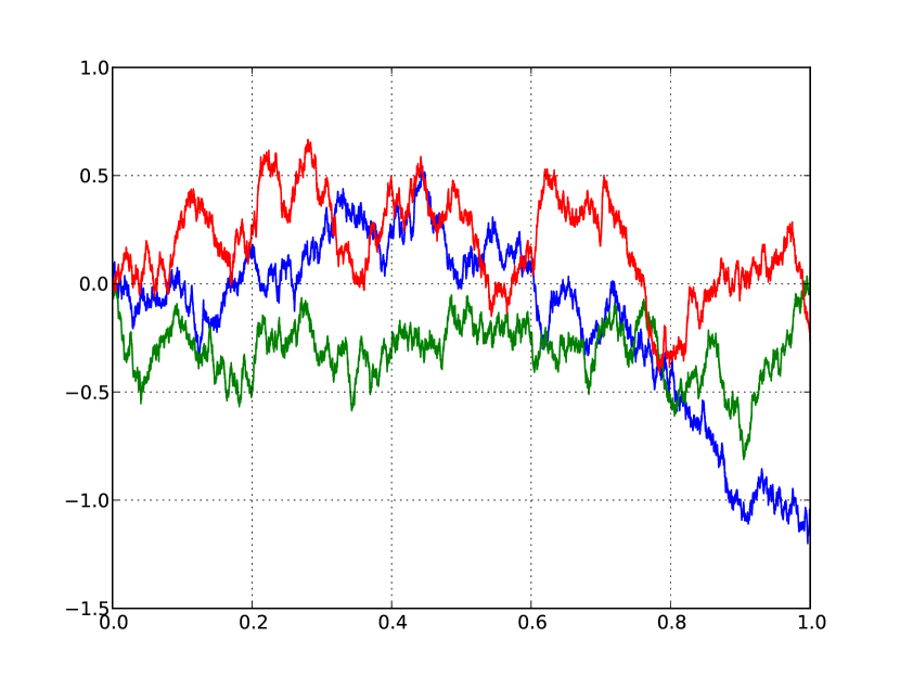
Figure 1: Sample paths of Brownian motion on the closed interval $[0,1]$ generated as described in the text using $\delta t=10^{-4}$.

Technicalities: It can be shown that a process is Brownian motion if and only if it is a continuous process with stationary and independent increments [12, p. 2]; these properties force the process to be Gaussian [13, Ch. 12], a consequence of the central limit theorem. Brownian motion, suitably scaled and with zero drift, is precisely the normalised, or standard, Brownian motion, described earlier. Had the $W(k)$ been replaced by any other distribution with zero mean and unit variance, the resulting process $X(t)$ still would have converged to Brownian motion as $\delta t\rightarrow 0$. Alternative methods for generating Brownian motion on the interval $[0,1]$ include truncating the Karhunen-Loève expansion, and successive refinements to the grid: $X(0)=0$, $X(1)\sim N(0,1)$, and given neighbouring points $X(t)$ and $X(t+\delta t)$, a mid-point is added by the rule $X(t+\frac{\delta t}{2})\sim\frac{X(t)+X(t+\delta t)}{2}+\frac{\sqrt{\delta t}}{2}N(0,1)$, thus allowing $X(\frac{1}{2})$ to be computed with $\delta t=1$, then $X(\frac{1}{4})$ and $X(\frac{3}{4})$ with $\delta t=\frac{1}{2}$ and so forth. Books specifically on Brownian motion include [14, 15, 16]. The origins of the mathematical concept of Brownian motion trace back to three independent sources; Thiele (1880), Bachelier (1900) and Einstein (1905). According to [17], “Of these three models, those of Thiele and Bachelier had little impact for a long time, while that of Einstein was immediately influential”.

II-B Brownian Motion and Stochastic Development

Nothing is lost for the moment by treating manifolds as “curved surfaces such as the circle or sphere”.

Brownian motion models a particle bombarded randomly by much smaller molecules. The recursion $X((k+1)\,\delta t)=X(k\,\delta t)+\sqrt{\delta t}\,W(k)$ introduced in Section II-A is thus (loosely) interpreted as a particle being bombarded at regular time instants. Between bombardments, there is no force acting on the particle, hence the particle’s trajectory must be a curve of zero acceleration. In Euclidean space, this implies particles move in straight lines between bombardments, and explains why linear interpolation was used earlier to connect $X(k\,\delta t)$ to $X((k+1)\,\delta t)$. On a manifold, a curve with zero acceleration is called a geodesic. Between bombardments, a particle on a manifold travels along a geodesic.

Conceptually then, a piecewise approximation to Brownian motion on a manifold can be generated essentially as before, just with straight-line motion replaced by geodesic motion.

Since the Earth is approximately a sphere, long-distance travel gives an intuitive understanding of the concepts of distance, velocity and acceleration of a particle moving on the surface of a sphere. Travelling “in a straight line” on the Earth actually means travelling along a great circle; great circles are the geodesics of the sphere.

There are different ways of understanding geodesics, but the most relevant for subsequent developments is the following: rolling a sphere, without slipping, over a straight line drawn in wet ink on a flat table will impart a curve on the sphere that precisely traces out a geodesic.

Rolling a manifold over a piecewise smooth curve in Euclidean space to obtain a curve on the manifold is called development. The development of a piecewise linear curve is a piecewise geodesic curve. If $x(t)=(x_{1}(t),x_{2}(t))$ is the piecewise linear approximation in Figure 2 of a realisation of two-dimensional Brownian motion then the developed piecewise geodesic curve obtained by rolling the sphere over the curve in Figure 2 is a piecewise geodesic approximation of a realisation of Brownian motion on the sphere.

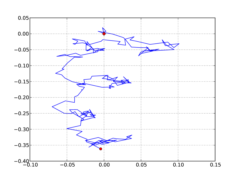
Figure 2: Path traced out by a very short segment of a single realisation of a two-dimensional Brownian motion starting from the diamond at the origin and stopping at the circle; $X(t)=(X_{1}(t),X_{2}(t))$ is two-dimensional Brownian motion if and only if $X_{1}(t)$ and $X_{2}(t)$ are one-dimensional Brownian motions independent of each other. Time has been omitted.

Development is defined mathematically as the solution of a certain differential equation. If a curve is not differentiable then it cannot be developed in the classical sense. A sample path of Brownian motion is nowhere differentiable! Therefore, in the first instance, development can only be used to take a piecewise smooth approximation of Brownian motion in Euclidean space and obtain a piecewise smooth approximation of Brownian motion on a manifold. Nevertheless, it is possible to “take limits” and develop a theory of stochastic development. The stochastic development of Brownian motion in Euclidean space is the limiting process obtained by developing successively more accurate piecewise smooth approximations of the Brownian motion in Euclidean space.

Technicality: This “smooth approximation” approach to stochastic development is more tedious to make rigorous than the stochastic differential equation approach taken in [6, Chapter 2] but offers more intuition for the neophyte.

The inverse of development is anti-development and can be visualised as drawing a curve on a manifold in wet ink and rolling the manifold along this curve on a table thereby leaving behind a curve on the table. Its stochastic counterpart, stochastic anti-development, can be thought of as the limiting behaviour of the anti-development of piecewise geodesic approximations of sample paths.

As a rule of thumb, techniques (such as filtering [18]) for processes on Euclidean space can be extended to processes on manifolds by using stochastic anti-development to convert the processes from manifold-valued to Euclidean-space-valued. Although this may not always be computationally attractive, it nevertheless affords a relatively simple viewpoint.

A process on a manifold is Brownian motion if and only if its stochastic anti-development is Brownian motion in Euclidean space [2, (8.26)]. To put this in perspective, note Brownian motion on a manifold cannot be defined using finite-dimensional distributions because there is no direct definition of a Gaussian random variable on a manifold. (Even disregarding the global topology of a manifold, a random variable which is Gaussian with respect to one chart need not be Gaussian with respect to another chart.) Much of the Euclidean-space theory relies on linearity, and the only linearity on manifolds is at the infinitesimal scale of tangent spaces. Stochastic development operates at the infinitesimal scale, replicating as faithfully as possible on a manifold a process in Euclidean space.

Although Gaussian random variables cannot be used to define Brownian motion on a manifold, the reverse is possible; Brownian motion can be used to generalise the definition of a Gaussian random variable to a manifold; see Section IX.

Technicalities: There are a number of characterisations of Brownian motion that can be used to generalise Brownian motion to manifolds, including as the unique Itô diffusion generated by the Laplace operator. The end result is nevertheless the same [19, 5, 20, 2, 21, 3, 6]. Whereas for deterministic signal processing, and in particular for optimisation on manifolds, there is benefit in not endowing a manifold with a Riemannian metric [22, 23], Brownian motion must be defined with respect to a Riemannian metric. Although some concepts, such as that of a semimartingale, can be defined on a non-Riemannian manifold, it is simplest here to assume throughout that all manifolds are Riemannian manifolds.

II-C The Geometry of the Sphere

This section continues the parallel threads of stochastic development and Brownian motion. Equations are derived for simulating Brownian motion on a sphere by rolling a sphere along a simulated path of Brownian motion in $\mathbb{R}^{2}$. It is convenient to change reference frames and roll a sheet of paper around a sphere than roll a sphere on a sheet of paper.

Exercise: Mentally or otherwise, take a sheet of graph paper and a soccer ball. Mark a point roughly in the middle of the graph paper as being the origin, and draw two unit-length vectors at right-angles to each other based at the origin. Place the origin of the graph paper on top of the ball. Roll the paper down the ball until arriving at the equator. Then roll the paper along the equator for some distance, then roll it back up to the top of the ball. Compare the orientation of the two vectors at the start and at the end of this exercise; in general, the orientation will have changed due to the curvature of the sphere. (Furthermore, in general, the origin of the graph paper will no longer be touching the top of the sphere.)

Throughout, any norm $\|\cdot\|$ or inner product $\langle\cdot,\cdot\rangle$ on $\mathbb{R}^{n}$ is the Euclidean norm or inner product. Perpendicular vectors are denoted $v\perp p$, meaning $\langle v,p\rangle=0$.

Take the sphere $S^{2}=\{(x_{1},x_{2},x_{3})\in\mathbb{R}^{3}\mid x_{1}^{2}+x_{2}^{2}+x_{3}^{2}=1\}$. Start the Brownian motion at the North pole: $B(0)=(0,0,1)$. Place a sheet of graph paper on top of the sphere, so the origin $(0,0)$ of the graph paper makes contact with the North pole $(0,0,1)$. Let $w_{1}(0)$ and $w_{2}(0)$ be realisations of independent $N(0,1)$ random variables. On the graph paper, draw a line segment from the origin $(0,0)$ to the point $(\sqrt{\delta t}\,w_{1}(0),\sqrt{\delta t}\,w_{2}(0))$; recall from Section II-A and Figure 2 that this is the first segment of an approximate sample path of Brownian motion on $\mathbb{R}^{2}$. The paper is sitting inside $\mathbb{R}^{3}$, and the point $(\sqrt{\delta t}\,w_{1}(0),\sqrt{\delta t}\,w_{2}(0))$ on the paper is actually located at the point $(\sqrt{\delta t}\,w_{1}(0),\sqrt{\delta t}\,w_{2}(0),1)$ in $\mathbb{R}^{3}$ because the paper is lying flat on top of the sphere.

Rolling the paper down the sphere at constant velocity along the line segment so it reaches the end of the segment at time $\delta t$ results in the point of contact between the paper and the sphere being given by

$$B(t)=\cos\left(\frac{t}{\delta t}\|v\|\right)p+\sin\left(\frac{t}{\delta t}\|v\|\right)\frac{v}{\|v\|}$$ (1)

for $t\in[0,\delta t]$, where $p=(0,0,1)$ is the original point of contact (the North pole) and $v=(\sqrt{\delta t}\,w_{1}(0),\sqrt{\delta t}\,w_{2}(0),0)$. This can be derived from first principles by requiring $B(t)$ to remain in a plane and have constant angular velocity.

In general, given any $p\in S^{2}$ and $v\perp p$, let $\operatorname{Exp}_{p}(v)$ denote the final contact point of the sphere and piece of paper obtained by starting with the paper touching the sphere at $p$, marking on the paper a line segment from $p$ to $p+v$, and rolling the paper over the sphere along that line. (Since $v\perp p$, and the paper is tangent to the sphere at $p$, the point $p+v$ will lie on the paper.) The curve $t\mapsto\operatorname{Exp}_{p}(tv)$ is a geodesic and follows a great circle. Explicitly, $\operatorname{Exp}_{p}(0)=p$ and, for $\|v\|\neq 0$,

$$\operatorname{Exp}_{p}(v)=\cos\left(\|v\|\right)p+\sin\left(\|v\|\right)\frac{v}{\|v\|}.$$ (2)

At the risk of belabouring the point, if $S^{2}$ represents the Earth and a person sets out from a point $p$ with initial velocity $v$ and continues “with constant velocity in a straight line” then his position at time $t$ will be $\operatorname{Exp}_{p}(tv)$. In detail, each step actually involves first taking a perfectly straight step in the tangent plane, meaning the leading foot will be slightly off the Earth, then without swivelling on the other foot, letting the force of gravity pull the leading foot down to the closest point on Earth. This is a discrete version of “rolling without slipping” and hence produces (or defines) a geodesic in the limit as smaller and smaller steps are taken.

The Riemannian exponential map $\operatorname{Exp}_{p}(v)$ can be defined analogously on any Riemannian manifold. The set of allowable velocities $v$ for which $\operatorname{Exp}_{p}(v)$ makes sense is called the tangent space to the manifold at the point $p$; just like for the sphere, the tangent space can be visualised as a sheet of paper providing the best linear approximation to the shape of the manifold in a neighbourhood of the point of contact and $v$ must be such that $p+v$ lies on this (infinitely large) sheet of paper. Alternatively, if a sufficiently small (or sufficiently short-sighted) ant were standing on the manifold at point $p$, so that the manifold looked flat, then the set of possible directions (with arbitrary magnitudes) the ant could set out in from his perspective forms the tangent space at $p$.

Technicalities: The Riemannian exponential function is defined via a differential equation. If the manifold is not complete, the differential equation may “blow up”; this technicality is ignored throughout the primer. Since every Riemannian manifold can be embedded in a sufficiently high-dimensional Euclidean space, this primer assumes for simplicity that all Riemannian manifolds are subsets of Euclidean space. The Riemannian geometry of such a manifold is determined by the Euclidean geometry of the ambient space; the Euclidean inner product induces an inner product on each tangent space. This is consistent with defining the length of a curve on a manifold as the Euclidean length of that curve when viewed as a curve in the ambient Euclidean space.

Returning to simulating Brownian motion on the sphere, recall the original strategy was to generate a Brownian motion on the plane then develop it onto the sphere. Carrying this out exactly would involve keeping track of the orientation of the paper as it moved over the sphere. Although this is easily done, it is not necessary for simulating Brownian motion because Gaussian random vectors are symmetric and hence invariant with respect to changes in orientation.

If a particle undergoing Brownian motion is currently at the point $p\in S^{2}$, its next position, after $\delta t$ units of time, can be simulated by generating a three-dimensional Gaussian random vector $v\sim N(0,I)\in\mathbb{R}^{3}$, projecting $v$ onto $T_{p}S^{2}$ — replace $v$ by $v-\langle v,p\rangle p$ — and declaring the next position of the particle to be $\operatorname{Exp}_{p}(\sqrt{\delta t}\,v)$. This generalises immediately to arbitrary manifolds and is summarised in Section II-E. (Alternatively, given an orthonormal basis for $T_{p}S^{2}$, a two-dimensional Gaussian random vector could have been used to generate an appropriate random element of $T_{p}S^{2}$.)

Although orientation was ultimately not needed for defining Brownian motion, it is an important concept by which to understand curvature, and enters the picture for more general processes (such as Brownian motion with drift).

Technicality: For a non-embedded manifold $M$, the natural setting for (stochastic) development is the frame bundle $\mathcal{F}(M)$ of $M$ equipped with a connection [6, 5, 3]. The connection decomposes the tangent bundle of $\mathcal{F}(M)$ into horizontal and vertical components, and leads to the concept of a horizontal process. A horizontal process on $\mathcal{F}(M)$ is essentially a process on $M$ augmented by its current orientation. If $M$ is Riemannian then the orthonormal frame bundle $\mathcal{O}(M)$ can be used instead of $\mathcal{F}(M)$. Horizontal Brownian motion can be defined on $\mathcal{O}(M)$ via a Stratonovich stochastic differential equation that stochastically develops Brownian motion in Euclidean space onto the horizontal component (with respect to the Levi-Civita connection) of $\mathcal{O}(M)$. The bundle projection of this horizontal Brownian motion yields Brownian motion on $M$.

II-D A Working Definition of a Riemannian Manifold

For the purposes of this primer, manifolds are defined as subsets of Euclidean space that are sufficiently nice to permit a useful theory of differentiation of functions from one such subset to another. (Furthermore, only $C^{\infty}$-smooth manifolds are discussed.) Conditions will be given for a subset $M\subset\mathbb{R}^{n}$ to be an $m$-dimensional manifold for some positive integer $m\leq n$. (A zero-dimensional manifold is a countable collection of isolated points and will not be considered further.) This will confirm the circle $S^{1}$ and sphere $S^{2}$ as manifolds of dimension one and two, respectively. Graphs of smooth functions are prototypical manifolds: if $f\colon\mathbb{R}^{m}\rightarrow\mathbb{R}^{n-m}$ is a smooth function, meaning derivatives of all orders exist, its graph $M=\{(x,f(x))\in\mathbb{R}^{m}\times\mathbb{R}^{n-m}\cong\mathbb{R}^{n}\mid x\in\mathbb{R}^{m}\}$ is an $m$-dimensional manifold.

For each point $p\in M$, define $T_{p}M$ as the set of all possible velocity vectors $\gamma^{\prime}(0)$ taken on by smooth curves $\gamma\colon\mathbb{R}\rightarrow\mathbb{R}^{n}$ whose images are wholly contained in $M$ and that pass through $p$ at time $0$. For example, if $p\in M=S^{2}$ then the (only) requirements on $\gamma$ are that it is smooth, that $\gamma(0)=p$ and $\|\gamma(t)\|=1$. In symbols,

$$T_{p}M=\{\gamma^{\prime}(0)\mid\gamma\colon\mathbb{R}\rightarrow\mathbb{R}^{n},\,\gamma(0)=p,\,\gamma(\mathbb{R})\subset M\}$$ (3)

where it is implicitly understood that $\gamma$ must be infinitely differentiable. (No difference results if $\gamma$ is only defined on an open neighbourhood of the origin; usually such curves are denoted $\gamma\colon(-\epsilon,\epsilon)\rightarrow M$ in the literature.)

The first requirement placed on $M$ is for it to look infinitesimally like $\mathbb{R}^{m}$. Precisely, it is required that $T_{p}M\subset\mathbb{R}^{n}$ is an $m$-dimensional vector subspace of $\mathbb{R}^{n}$ for every $p\in M$. This prevents $M$ from having (non-tangential) self-intersections, e.g., the letter $X$ is not a manifold, and it prevents $M$ from having cusps, e.g., the letter $V$ is not a manifold because no smooth curve $\gamma$ passes through the bottom tip of $V$ except for the constant curve with $\gamma^{\prime}(0)=0$.

Usually this first requirement is not stated because it is subsumed by requiring the manifold be locally Euclidean, defined presently. Nevertheless, it emphasises the importance of tangent spaces. The visual image of a piece of paper placed against a sphere at the point $p\in S^{2}\subset\mathbb{R}^{3}$ is the affine tangent space. The tangent space $T_{p}S^{2}$ is obtained by taking the piece of paper and translating it to pass through the origin of the ambient space $\mathbb{R}^{3}$. This distinction is usually blurred.

The first requirement fails to disqualify the figure of eight from being a manifold because it cannot detect tangential self-intersections. This can only be detected by considering what is happening in a neighbourhood of each and every point; it is required that for all $p\in M\subset\mathbb{R}^{n}$ there exists a sufficiently small open ball $B_{r}(p)=\{z\in\mathbb{R}^{n}\mid\|z-p\|<r\}$ of radius $r>0$ and a diffeomorphism $h\colon\mathbb{R}^{n}\rightarrow B_{r}(p)$, meaning $h$ is bijective and both $h$ and its inverse are smooth, such that

$$h(\mathbb{R}^{m}\times\{0\})=B_{r}(p)\cap M$$ (4)

where $\mathbb{R}^{m}\times\{0\}=\{(x,0)\in\mathbb{R}^{n}\mid x\in\mathbb{R}^{m}\}$ is the embedding of $\mathbb{R}^{m}$ into $\mathbb{R}^{n}$ obtained by setting the last $n-m$ coordinates equal to zero. (The basic intuition is that the classical calculus on a flat subspace $\mathbb{R}^{m}\times\{0\}$ of $\mathbb{R}^{n}$ should be extendable to a calculus on diffeomorphic images of this flat subspace.)

The restriction of $h$ in (4) to $\mathbb{R}^{m}\times\{0\}$ is a parametrisation of a part of the manifold $M$, however, the condition is stronger than this since it requires the parametrisation include all points of $M$ in $B_{r}(p)\cap M$ and no other points. This excludes the figure “8” because at the point where the top and bottom circles meet, every one-dimensional parametrisation can get at best only part of the lower hemisphere of the top circle and the upper hemisphere of the bottom circle. In fact, (4) ensures that every manifold locally looks like a rotated graph of a smooth function.

A manifold $M\subset\mathbb{R}^{n}$ inherits a Riemannian structure from the Euclidean inner product on $\mathbb{R}^{n}$. This leads to defining the acceleration of a curve $\gamma\colon\mathbb{R}\rightarrow M\subset\mathbb{R}^{n}$ at time $t$ as $\pi_{\gamma(t)}\left(\gamma^{\prime\prime}(t)\right)$ where $\pi_{p}\colon\mathbb{R}^{n}\rightarrow T_{p}M$ is orthogonal projection onto $T_{p}M$. The curve $\gamma$ is a geodesic if and only if $\gamma^{\prime\prime}(t)$ contains only those vectorial components necessary to keep the curve on the manifold, that is, $\pi_{\gamma(t)}\left(\gamma^{\prime\prime}(t)\right)=0$ for all $t$. This same condition could have been deduced by developing a straight line onto $M$, as in Section II-B.

Technicalities: On a non-Riemannian manifold, there is a priori no way of defining the acceleration of a curve because there is no distinguished way of aligning $T_{p}M$ and $T_{q}M$ for two distinct points $p$ and $q$. The above definition implicitly uses the Riemannian structure coming from the ambient space $\mathbb{R}^{n}$ and accords with comparing tangent vectors at two distinct points of a curve by placing a piece of paper over the manifold at point $q$, drawing the tangent vector at $q$ on the piece of paper, then rolling the paper to $p$ along the curve, and drawing the tangent vector at $p$ on the paper. Because the piece of paper represents Euclidean space, the base points of the vectors drawn on the paper can be translated in the usual way so that they align. This then allows the difference of the two vectors to be taken, and ultimately, allows the acceleration to be defined as the rate of change of the velocity vectors. A mechanism for aligning neighbouring affine tangent spaces along a curve is called an affine connection. The particular affine connection described here is the Levi-Civita connection, the unique torsion-free connection that is compatible with the Riemannian metric. In more advanced settings, there may be advantages to using other affine connections. A limitation of insisting manifolds are subsets of Euclidean space is that changing to a different metric requires changing the embedding, for example, changing the sphere into an ellipse.

II-E Brownian Motion on Manifolds

Assembling the pieces leads to the following algorithm for simulating Brownian motion on an $m$-dimensional Riemannian manifold $M\subset\mathbb{R}^{n}$.

Choose a starting point on $M$; set $B(0)$ to this point. Fix a step size $\delta t>0$. For $k=0,1,\cdots$, recursively do the following. Generate a Gaussian random vector $W(k)\in T_{B(k\,\delta t)}M\subset\mathbb{R}^{n}$, either with the help of an orthonormal basis for $T_{B(k\,\delta t)}M$, or by generating an $n$-dimensional $N(0,I)$ Gaussian random vector and projecting the vector orthogonally onto $T_{B(k\,\delta t)}M$ to obtain $W(k)$. Then define

$$B(k\,\delta t+t)=\operatorname{Exp}_{B(k\,\delta t)}\left(\frac{t}{\delta t}\sqrt{\delta t}\,W(k)\right).$$ (5)

for $t\in[0,\delta t]$. If $M=\mathbb{R}^{n}$ then $\operatorname{Exp}_{p}(v)=p+v$ and (5) agrees with the algorithm in Section II-A.

Technicality: An advantage of projecting orthogonally onto the tangent space rather than constructing an orthonormal basis is that while the orthogonal projection $\pi_{p}\colon\mathbb{R}^{n}\rightarrow T_{p}M$ varies smoothly in $p$, on non-parallelisable manifolds it is not possible to find a continuous mapping from $p\in M$ to an orthonormal basis of $T_{p}M$. The hairy ball theorem implies that the sphere $S^{2}$ is not parallelisable. (In fact, in terms of spheres, only $S^{0}$, $S^{1}$, $S^{3}$ and $S^{7}$ are parallelisable.)

It is verified in [24] that, as $\delta t\rightarrow 0$, the above approximation converges in distribution to Brownian motion, where Brownian motion is defined by some other means. (For the special case of Lie groups, see also [25]. For hypersurfaces, see [26].) Nevertheless, engineers (and physicists) may find it attractive to treat the limit of (5) as the definition of Brownian motion. All (5) is saying is that at each step, movement in any direction is equally likely and independent of the past. By the central limit theorem, it suffices for the $W(k)$ to have zero mean and unit variance; see [27] for an analysis of an algorithm commonly used in practice. The presence of the square root in the term $\sqrt{\delta t}$ is easily explained by the compatibility requirement that the variance of $B(T)$ generated using a step size of $\delta t$ be equal to the variance of $B(T)$ generated using a step size of $\frac{\delta t}{2}$; if this were not so then the processes need not converge as $\delta t\rightarrow 0$.

While (5) is suitable for numerical work, for calculations by hand it is convenient to “take limits” and work with the actual process. A direct analogy is preferring to work with $\frac{dx}{dt}$ rather than $\frac{x(t+\delta t)-x(t)}{\delta t}$. Section IV introduces a stochastic calculus.

III State-Space Models on Manifolds

III-A Motivation

Signal processing involves generating new processes from old. In Euclidean space, a process can be passed through a linear time-invariant system to obtain a new process. This can be written in terms of an integral and motivates asking if a continuous-time process evolving on a manifold, such as Brownian motion, can be integrated to obtain a new process.

Another obvious question is how to generalise to manifolds state-space models with additive noise. The classical linear discrete-time state-space model is

$$X_{k+1} =A_{k}X_{k}+B_{k}V_{k},$$ (6)

$$Y_{k} =C_{k}X_{k}+D_{k}W_{k}$$ (7)

where $A_{k},B_{k},C_{k},D_{k}$ are matrices and $V_{k},W_{k}$ are random vectors (noise). The vector $X_{k}$ is the state at time $k$, and the state-space equation represents the dynamics governing how the state changes over time. It comprises a deterministic part $A_{k}X_{k}$ and a stochastic part $B_{k}V_{k}$. The second equation is the observation equation: the only measurement of the state available at time $k$ is the vector $Y_{k}$ comprising a linear function of the state and additive noise.

There does not appear to be a natural generalisation of discrete-time state-space models to arbitrary manifolds because it is not clear how to handle the addition of the two terms in each equation. (In some cases, group actions could be used.) It will be seen presently that continuous-time state-space models generalise more easily. This suggests the expediency of treating discrete-time processes as sampled versions of continuous-time processes.

The continuous-time version of (6) would be

$$\frac{dX}{dt}=A(t)X(t)+B(t)\frac{dV(t)}{dt}$$ (8)

if the noise process $V(t)$ was sufficiently nice that its sample paths were absolutely continuous; that this generally is not the case is ignored for the moment.

Although $Y(t)=C(t)X(t)+D(t)W(t)$ is an analogue of (7), usually the observation process takes instead the form

$$\frac{dY}{dt}=C(t)X(t)+D(t)\frac{dW(t)}{dt}$$ (9)

which integrates rather than instantaneously samples the state.

Although the right-hand sides of (6) and (8) are sums of two terms, crucially, it is two tangent vectors being summed in (8). Two points on a manifold cannot be added but two tangent vectors in the same tangent space can. Therefore, (8) and (9) extend naturally to manifolds provided the terms $A(t)X(t)$ and $C(t)X(t)$ are generalised to be of the form $b(t,X(t))$; see (10). The challenge is if $V(t)$ and $W(t)$ are Brownian motion then (8) and (9) require an appropriate interpretation because Brownian motion is nowhere differentiable (almost surely). The following subsections hint at how this is done via piecewise approximations, and Section IV gives a rigorous interpretation by changing (8) and (9) to integral form.

III-B Modelling the State Process

Building on the material in Sections II and III-A, an attempt is made to model a particle moving on a sphere subject to disturbance by Brownian motion. Let $X(t)\in S^{2}\subset\mathbb{R}^{3}$ denote the position of the particle at time $t$. Its deterministic component can be specified by a differential equation

$$\frac{dX}{dt}=b(t,X(t)).$$ (10)

Provided $b(t,X(t))$ lies in the tangent space of the sphere at $X(t)$, the solution of (10) is forced to lie on the sphere if the initial point $X(0)$ does. A simple numerical solution of (10) is obtained by combining the forward-Euler method with the Riemannian exponential function, the latter ensuring the approximate solution remains on the sphere:

$$X(t+\delta t)=\operatorname{Exp}_{X(t)}\big{(}\delta t\,b(t,X(t))\big{)}.$$ (11)

Referring to (5) with $t=\delta t$, the following idea presents itself:

$$X(t+\delta t)=\operatorname{Exp}_{X(t)}\big{(}\delta t\,b(t,X(t))+\sqrt{\delta t}\,W(t)\big{)}$$ (12)

where $W(t)$ is an $N(0,I)$ Gaussian random vector in $\mathbb{R}^{3}$ projected orthogonally onto the tangent space $T_{X(t)}S^{2}$. The (approximately instantaneous) velocity of the particle at time $t$ is the sum of a deterministic component and a random component. Continuous-time approximations can be obtained by interpolating using geodesics, as in (5), in which case (12) converges to a well-defined process on the sphere [28].

III-C Modelling the Observation Process

Notwithstanding that the first two cases are subsumed by the third, the three cases of interest are: the state process evolves in Euclidean space yet the observation process is manifold-valued; the state process evolves on a manifold but the observation process is real-valued; and, the state and observation processes are manifold-valued.

If the state process $X(t)$ evolves in Euclidean space then stochastic development can be used to feed it into the observation process [28]:

$$Y(t+\delta t)=\operatorname{Exp}_{Y(t)}\big{(}X(t+\delta t)-X(t)+\sqrt{\delta t}\,W(t)\big{)}.$$ (13)

If $X(t)$ is not observed directly, but only $g(X(t))$ where $g$ is a smooth function between Euclidean spaces, then a straightforward modification of (13) is

$$Y(t+\delta t)=\operatorname{Exp}_{Y(t)}\big{(}g(X(t+\delta t))-g(X(t))+\sqrt{\delta t}\,W(t)\big{)}.$$ (14)

In other words, first the new process $\tilde{X}(t)=g(X(t))$ is formed, then noise is added to it, and finally it is stochastically developed (via piecewise approximations) onto the manifold.

If the state process $X(t)$ evolves on a manifold of dimension $m$ but the observation process $Y(t)$ is real-valued then stochastic anti-development can be used [29]. In a sufficiently small domain, $\operatorname{Exp}$ is invertible, and the instantaneous velocity of $X(t)$, which in general does not exist, can nevertheless be approximated by $\operatorname{Exp}^{-1}_{X(t)}\big{(}X(t+\delta t)-X(t)\big{)}$. This produces a vector in $\mathbb{R}^{m}$ which can be used to update an observation process evolving in Euclidean space. (By interpreting differential equations as integral equations, as discussed in Section IV, neither $X(t)$ nor $Y(t)$ need be differentiable for there to be a well-defined limiting relationship between the instantaneous velocities of piecewise approximations of the processes.)

Finally, the general case of both $X(t)$ and $Y(t)$ evolving on manifolds falls under the framework of stochastic differential equations between manifolds [30, Section 3]. Basically, $\operatorname{Exp}^{-1}_{X(t)}$ can be used to obtain a real-valued vector approximating the instantaneous velocity of $X(t)$, which after a possible transformation, can be fed into $\operatorname{Exp}_{Y(t)}$ to update the observation process $Y(t)$. See [2] for details.

III-D Discussion

Section III demonstrated, at least on an intuitive level, that stochastic development and anti-development, and the $\operatorname{Exp}$ map in particular, provide a relatively straightforward way of generalising state-space models to manifolds.

Nevertheless, it is important to understand what the limiting processes are that $\operatorname{Exp}$ is being used to approximate. This is the purpose of stochastic calculus, and once it is appreciated that the “smooth approximation” approach discussed in this primer leads to a stochastic calculus, it is generally easier to use directly the stochastic calculus.

IV Stochastic Calculus and Itô Diffusions

This section does not consider manifolds or processes with jumps [31]. Standard references include [32, 10].

IV-A Background

A generalisation of (10) is the functional equation

$$X(t)=X(0)+\int_{0}^{t}b(s,X(s))\,ds.$$ (15)

A solution of (15) is any function $X(t)$ for which both sides of (15) exist and are equal. Every solution of (10) is a solution of (15) but the converse need not hold; whereas $X(t)$ must be differentiable for the left-hand side of (10) to make sense, there is no explicit differentiability requirement in (15), only the requirement that $b(s,X(s))$ be integrable.

The same idea carries over to random processes; although Brownian motion cannot be differentiated, it can be used as an integrator, and the state-space equations (8) and (9) can be written rigorously as functional equations by integrating both sides. However, there is in general no unique way of defining the integral of a process.

Since it may come as a surprise that different definitions of integrals can give different answers, this phenomena will be illustrated in the deterministic setting by considering how to integrate Hölder continuous functions of order $\tfrac{1}{2}$. Such functions are continuous but may oscillate somewhat wildly.

Technicality: Although sample paths of Brownian motion are almost surely not Hölder continuous of order $\tfrac{1}{2}$, they are almost surely Hölder continuous of any order less than $\tfrac{1}{2}$. This is irrelevant here because, as explained below, the relevant fact about Brownian motion is that $\mathbb{E}\left[{|B(t+\delta t)-B(t)|}\right]$ is proportional to $\sqrt{\delta t}$ rather than $\delta t$. The appearance of the expectation operator characterises the stochastic approach to integration. Interestingly, a complementary theory known as rough paths has been developed recently [33, 34, 35, 36], based partially on observations made in [37, 38] and [39].

Recall the Riemann-Stieltjes integral $\int_{0}^{1}f(s)\,dg(s)$ which, for smooth $f$ and $g$, is a limit of Riemann sums:

$$\int_{0}^{1}f(s)\,dg(s)=\lim_{N\rightarrow\infty}\sum_{k=0}^{N-1}f(\tfrac{k}{N})\left(g(\tfrac{k+1}{N})-g(\tfrac{k}{N})\right).$$ (16)

The right-hand side of (16) gives the same answer if the right, not left, endpoint is used for each interval $[\frac{k}{N},\frac{k+1}{N}]$. Indeed, the difference between using left or right endpoints is

$$e_{N}=\sum_{k=0}^{N-1}\left(f(\tfrac{k+1}{N})-f(\tfrac{k}{N})\right)\left(g(\tfrac{k+1}{N})-g(\tfrac{k}{N})\right).$$ (17)

If $f$ is smooth then $|f(\tfrac{k+1}{N})-f(\tfrac{k}{N})|\leq\alpha_{f}\tfrac{1}{N}$ for some constant $\alpha_{f}\in\mathbb{R}$, and analogously for $g$. Therefore, $|e_{N}|\leq\alpha_{f}\alpha_{g}\sum_{k=0}^{N-1}\tfrac{1}{N}\,\tfrac{1}{N}$ and converges to zero as $N\rightarrow\infty$.

If now $f$ and $g$ are not differentiable, but merely Hölder continuous of order $\tfrac{1}{2}$, then $|f(\tfrac{k+1}{N})-f(\tfrac{k}{N})|\leq\alpha_{f}|\tfrac{1}{N}|^{\tfrac{1}{2}}$ for some constant $\alpha_{f}\in\mathbb{R}$, and analogously for $g$, leading to $|e_{N}|\leq\alpha_{f}\alpha_{g}\sum_{k=0}^{N-1}|\tfrac{1}{N}|^{\tfrac{1}{2}}\,|\tfrac{1}{N}|^{\tfrac{1}{2}}$ which converges to $\alpha_{f}\alpha_{g}$, and not zero, as $N\rightarrow\infty$. This means it is possible for two different values of the integral $\int_{0}^{1}f(s)\,dg(s)$ to be obtained depending on whether $f(\tfrac{k}{N})$ or $f(\tfrac{k+1}{N})$ is used in (16).

If at least one of $f$ or $g$ is smooth and the other is Hölder continuous of order $\tfrac{1}{2}$ then once again $|e_{N}|\rightarrow 0$.

If $g$ is replaced by real-valued Brownian motion $B(t)$ and the above calculations carried out, a relevant quantity is the rate at which the expected value of $|B(t+\delta t)-B(t)|$ decays to zero. Since $B(t+\delta t)-B(t)\sim N(0,\delta t)$, $\mathbb{E}\left[{|B(t+\delta t)-B(t)|}\right]$ is proportional to $\sqrt{\delta t}$, analogous to $|f(t+\delta t)-f(t)|\propto\sqrt{\delta t}$ for Hölder continuous functions of order $\tfrac{1}{2}$. Not surprisingly then, differences can appear for integrals of the form $\int X(t)\,dY(t)$ when $X(t)$ and $Y(t)$ are stochastic processes; other integrals, such as $\int X(t)\,dt$ and $\int h(t)\,dY(t)$, with $h$ smooth, are unambiguous. (This presupposes $X(t)$ and $Y(t)$ are semimartingales [40].)

Technicalities: Lebesgue-Stieltjes theory requires finite variation, excluding Brownian motion as an integrator. Hölder continuous functions of order greater than $\tfrac{1}{2}$ can be integrated with respect to Lipschitz functions using the Young integral without needing finite variation [41]. Brownian motion falls just outside this condition. Stochastic integration theory depends crucially on integrators having nice statistical properties for Riemann-sum approximations to converge; see Section VI-A. The sums are sensitive to second-order information (cf. Itô’s formula [10]), hence “second-order calculus” is fundamental to stochastic geometry [2, Section VI].

IV-B Itô and Stratonovich Integrals: An Overview

Non-equivalent definitions of stochastic integrals [42, 43] all involve taking limits of approximations but differ in the approximations used and the processes that are allowed to be integrators and integrands. The two most common stochastic integrals are the Itô and Stratonovich integrals.

The Itô integral leads to a rich probabilistic theory based on a class of processes known as semimartingales, and a resulting stochastic analysis that, in some ways, parallels functional analysis. A tenet of analysis is that properties of a function $f(t)$ can be inferred from its derivative; for example, a bound on $f(T)$ can be derived from bounds on $f^{\prime}(t)$ because $f(T)=\int_{0}^{T}f^{\prime}(t)\,dt$. (It is remarkable how often it is easier to study an infinite number of linear problems, namely, examining $f^{\prime}(t)$ for each and every $t$ in the range $0$ to $T$.) Thinking of the random variable $X(T)$ as an infinite sum of its infinitesimal differences — $X(T)=\int_{0}^{T}dX(t)$ — suggests that by understanding the limiting behaviour of $X(t+\delta t)-X(t)$ as $\delta t\rightarrow 0$, it is possible to infer properties of $X(T)$ that may otherwise be difficult to infer directly.

Technicality: If the decomposition $Y(T)=\int_{0}^{T}dY(t)$ of $Y(t)=f(X(t))$ is sought, the Itô formula allows the limiting behaviour of $Y(t+\delta t)-Y(t)$ to be determined directly from the limiting behaviour of $X(t+\delta t)-X(t)$.

The Itô integral does not respect geometry [2]; it does not transform “correctly” to allow a coordinate-independent definition. Nor does the Itô integral respect polygonal approximations: if $Y^{k}(t)$ is a sequence of piecewise linear approximations converging to $Y(t)$ then it is not necessarily true that $\int X(t)\,dY^{k}(t)\rightarrow\int X(t)\,dY(t)$.

The Stratonovich integral lacks features of the Itô integral but respects geometry and polygonal approximations, making it suitable for stochastic geometry and modelling physical phenomena. Fortunately, it is usually possible to convert from one to the other by adding a correction term, affording freedom to choose the simpler for the calculation at hand.

By respecting geometry, the Stratonovich integral behaves like its deterministic counterpart; this is the transfer principle. The archetypal example is that the trajectory $X(t)$ of a Stratonovich stochastic differential equation $dX(t)=f(t,X(t))\circ dB(t)$ stays on a manifold $M$ if $f(t,X(t))$ lies in the tangent space $T_{X(t)}M$; cf. (10).

In terms of modelling, the Itô integral is suitable for approximating inherently discrete-time systems by continuous-time systems (e.g., share trading), while the Stratonovich integral is suited to continuous-time physical processes because it describes the limit of piecewise smooth approximations [44].

Technicality: On a non-Riemannian manifold, a Stratonovich integral but not an Itô integral can be defined because only the former respects geometry. Only once a manifold is endowed with a connection can an Itô integral be defined.

IV-C Semimartingales and Adapted Processes

The class of processes called semimartingales emerged over time by attempts to push Itô’s theory of integration to its natural limits. Originally defined as “adapted càdlàg processes decomposable into the sum of a local martingale and a process of finite variation”, the Bichteler-Dellacherie theorem [45, 46] states that semimartingales can be defined alternatively (in a simple and precise way [4]) as the largest class of “reasonable integrators” around which can be based a powerful and self-contained theory of Itô stochastic integration [40].

Note: Càdlàg and càglàd processes [40] generalise continuous processes by permitting “well-behaved” jumps.

Technicality: By restricting the class of integrands, the class of integrators can be expanded beyond semimartingales, leading to an integration theory for fractional Brownian motion, for example. Nevertheless, the Itô theory remains the richest.

From an engineering perspective, primary facts are: all Lévy processes [47], including the Poisson process and Brownian motion, are semimartingales, as are all (adapted) processes with continuously differentiable sample paths, and if a semimartingale is passed into a system modelled by an Itô integral, the output will also be a semimartingale. From an analysis perspective, semimartingales are analogues of differentiable functions in that a process $X(t)$ can be written, and studied, in terms of its differentials $dX(t)$; see Section IV-B. (Whereas the differential of a smooth function captures only first-order information, the Schwartz principle [2, (6.21)] is that $dX(t)$ captures both first-order and second-order information. This is stochastic information though; sample paths of semimartingales need not be differentiable.)

Crucial to Itô’s development of his integral was the restriction to adapted processes: in $\int X\,dY$, Itô required $X(\tau)$ not to depend on $Y(t)$ for $t\geq\tau$. (The borderline case $t=\tau$ results in Itô’s requirement that $X$ be càglàd and $Y$ càdlàg.) A filtration formalises what information has been revealed up to any given point in time. Adaptedness to the filtration at hand is a straightforward technical condition [10] taken for granted, and hence largely ignored, in this primer.

IV-D The Itô and Stratonovich Integrals

Let $X(t)$ be a continuous process and $Y(t)$ a semimartingale (both adapted to the same filtration). The Itô integral

$$Z(t)=\int_{0}^{t}X(s)\,dY(s)$$ (18)

can be interpreted as a system with transfer function $X(t)$ that outputs the semimartingale $Z(t)$ in response to the input $Y(t)$.

By [40, Theorem II.21], (18) is the limit (in probability)

$$Z(t)=\lim_{N\rightarrow\infty}\sum_{k=0}^{N-1}X(t_{k})\big{(}Y(t_{k+1})-Y(t_{k})\big{)}$$ (19)

where $t_{k}=\tfrac{k}{N}t$. (The Itô integral naturally extends to adapted càglàd integrands. This suffices for stochastic differential equations. With effort, further extensions are possible [40].)

The Stratonovich integral [48] is denoted

$$Z(t)=\int_{0}^{t}X(s)\circ dY(s).$$ (20)

It can be thought of as the limit (in probability)

$$Z(t)=\lim_{N\rightarrow\infty}\sum_{k=0}^{N-1}X(\tau_{k})\big{(}Y(t_{k+1})-Y(t_{k})\big{)}$$ (21)

where $t_{k}=\tfrac{k}{N}t$ and $\tau_{k}=\frac{t_{k}+t_{k+1}}{2}$. Alternatively, it can be evaluated as a limit of ordinary integrals. Define the piecewise linear approximation

$$Y^{\delta}(k\,\delta+t)=(1-t)\,Y(k\,\delta)+t\,Y((k+1)\,\delta)$$ (22)

for $t\in[0,1]$ and non-negative integers $k$. (For notational convenience, $\delta$ is being used here instead of $\delta t$.) Then

$$Z^{\delta}(t)=\int_{0}^{t}X(s)\,dY^{\delta}(s)$$ (23)

is a well-defined ordinary integral, and $Z^{\delta}(t)\rightarrow Z(t)$ as $\delta\rightarrow 0$. By differentiating $Y^{\delta}(s)$, (23) becomes

$$Z^{\delta}(t)=\sum_{k=0}^{N-1}\tfrac{Y((k+1)\delta)-Y(k\delta)}{\delta}\int_{k\delta}^{(k+1)\delta}X(s)\,ds$$ (24)

where $\delta=\tfrac{t}{N}$. This agrees in the limit with (21) whenever $\frac{1}{\delta}\int_{k\delta}^{(k+1)\delta}X(s)\,ds\rightarrow X(\tau_{k})$ where $\tau_{k}=(k+\tfrac{1}{2})\delta$.

Note: In the one-dimensional case, other reasonable approximations can be used. However, in general (i.e., when non-commuting vector fields are involved), failure to use piecewise linear approximations can lead to different answers [30].

Technicality: Unlike for the Itô integral, it is harder to pin down conditions for the Stratonovich integral to exist. This makes the definition of the Stratonovich integral a moving target. It is generally preferable to use (21) with $X(\tau_{k})$ replaced by $\tfrac{1}{2}(X(t_{k})+X(t_{k+1}))$; the modified sum apparently converges under milder conditions [49]. Alternatively, [50] declares the Stratonovich integral to exist if and only if the polygonal approximations with respect to all (not necessarily uniform) grids converge in probability to the same limit, the limit then being taken to be the value of the integral. For reasonable processes though, these definitions coincide.

IV-E Stochastic Differential Equations

The stochastic differential equation

$$dX(t)=b(t,X(t))\,dt+\Sigma(t,X(t))\,dB(t)$$ (25)

is shorthand notation for the functional equation

$$X(t)=X(0)+\int_{0}^{t}b(s,X(s))\,ds+\int_{0}^{t}\Sigma(s,X(s))\,dB(s)$$ (26)

which asks for a semimartingale $X(t)$ such that both sides of (26) are equal. In higher dimensions, the diffusion coefficient $\Sigma$ is a function returning a matrix and the drift $b$ a function returning a vector.

The Itô equation (26) can be solved numerically by a standard forward-Euler method (known in the stochastic setting as the Euler-Maruyama method) [51, 52, 53, 54, 55]. This validates the otherwise ad hoc models developed in Section III.

Replacing the Itô integral by the Stratonovich integral results in a Stratonovich stochastic differential equation. Since the summation in (21) involves evaluating $X(t)$ at a point in the future — the midpoint of the interval rather than the start of the interval — solving a Stratonovich equation necessitates either using an implicit integration scheme (such as a predictor-corrector method) or converting the Stratonovich equation into an Itô equation by adding a correction to the drift coefficient [52, 56, 53, 54, 55]. For example, in the one-dimensional case, solutions of the Stratonovich equation

$$dX(t)=\sigma(t,X(t))\circ dB(t)$$ (27)

correspond to solutions of the Itô equation

$$dX(t)=\tfrac{1}{2}\sigma(t,X(t))\,\frac{\partial\sigma}{\partial X}(t,X(t))\,dt+\sigma(t,X(t))\,dB(t).$$ (28)

IV-F Itô Diffusions

A process $X(t)$ is an Itô diffusion if it can be written in the form (26) where $B(t)$ is Brownian motion. (In fact, Itô developed his stochastic integral in order to write down directly continuous Markov processes based on their infinitesimal generators [57].) Stratonovich equations of the analogous form are also Itô diffusions. Itô diffusions are particularly nice to work with as they have a rich and well-established theory.

Technicality: The class of continuous Markov processes should be amongst the simplest continuous-time processes to study since local behaviour presumably determines global behaviour. Surprisingly then, even restricting attention to strongly Markov processes (thus ensuring the Markov property holds also at random stopping times) does not exclude complications, especially in dimensions greater than one [21, Section IV.5]. The generic term “diffusion” is used with the aim of restricting attention to an amenable subclass of continuous strongly Markov processes. Often this results in diffusions being synonymous with Itô diffusions but sometimes diffusions are more general.

V From Euclidean Space To Manifolds

Section III used piecewise geodesic approximations to define state-space models on manifolds. These approximations converge to solutions of stochastic differential equations. Conversely, one way to understand Stratonovich differential equations on manifolds is as limits of ordinary differential equations on manifolds applied to piecewise geodesic approximations of sample paths [2, Theorem 7.24].

Stratonovich equations on a manifold $M$ can be defined using only stochastic calculus in Euclidean space. A class of candidate solutions is needed: an $M$-valued process $X_{t}$ is a semimartingale if the “projected” process $f(X_{t})$ is a real-valued semimartingale for every smooth $f\colon M\rightarrow\mathbb{R}$; a shift in focus henceforth makes the notation $X_{t}$ preferable to $X(t)$. A Stratonovich equation on $M$ gives a rule for $dX_{t}$ in terms of $X_{t}$ and a driving process. Whether a semimartingale $X_{t}$ is a solution can be tested by comparing $df(X_{t})$ with what it should equal according to the stochastic chain rule; cf. (35). If this test passes for every smooth $f\colon M\rightarrow\mathbb{R}$ then $X_{t}$ is deemed a solution [6, Definition 1.2.3].

The following subsections touch on other ways of working with stochastic equations on manifolds.

V-A Local Coordinates

Manifolds are formally defined via a collection of charts composing an atlas [58]. (Charts were not mentioned in Section II-D but exist by the implicit function theorem.) A direct analogy is the representation of the Earth’s surface by charts (i.e., maps) in a cartographer’s atlas. Working in local coordinates means choosing a chart — effectively, a projection of a portion of the manifold onto Euclidean space — and working with the projected image in Euclidean space using Cartesian coordinates. This is the most fundamental way of working with functions or processes on manifolds.

A clear and concise example of working with stochastic equations in local coordinates is [59]. When written in local coordinates, stochastic differential equations on manifolds are simply stochastic differential equations in Euclidean space.

Working in local coordinates requires ensuring consistency across charts. When drawing a flight path in a cartographer’s atlas and nearing the edge of one page, changing to another page necessitates working with both pages at once, aligning them on their overlap. For theoretical work, this is usually only a minor inconvenience. The inconvenience may be greater for numerical work.

V-B Riemannian Exponential Map

On a general manifold there is no distinguished choice of local coordinates; all compatible local coordinates are equally valid. On a Riemannian manifold though, the Riemannian exponential map gives rise to distinguished local parametrisations of the manifold, the inverses of which are local coordinate systems called normal coordinates. The Riemannian exponential map has a number of attractive properties. It plays a central role in the smooth approximation approach to stochastic development, and has been used throughout this primer to generalise Brownian motion and stochastic differential equations to manifolds.

The main disadvantage of the Riemannian exponential map is that, in general, it cannot be evaluated in closed form, and its numerical evaluation may be significantly slower than working instead with extrinsic coordinates or even other local coordinate systems.

V-C Extrinsic Coordinates

Stochastic equations on manifolds embedded in Euclidean space can be written as stochastic equations in Euclidean space that just so happen to have solutions lying always on the manifold; see Section VII.

Even though all manifolds are embeddable in Euclidean space, there is no reason to expect an arbitrary manifold to have an embedding in Euclidean space that is convenient to work with (or even possible to describe). The dimension of the embedding space may be considerably higher than the dimension of the manifold, making for inefficient numerical implementations. Numerical implementations may be prone to “falling off the manifold”, or equivalently, incur increased computational complexity by projecting the solution back to the manifold at each step. (Falling off the manifold is only a numerical concern because the transfer principle makes it easy to constrain solutions of Stratonovich equations in $\mathbb{R}^{n}$ to lie on a manifold $M\subset\mathbb{R}^{n}$; see Section IV-B.)

Technicality: Given the use of Grassmann manifolds in signal processing applications, it is remarked there is an embedding of Grassmann manifolds into matrix space given by using orthogonal projection matrices to represent subspaces.

V-D Intrinsic Operations

Differential geometry is based on coordinate independence. On a Riemannian manifold, the instantaneous velocity and acceleration of a curve have intrinsic meanings understandable without reference to any particular coordinate system. Similarly, stochastic operators can be defined intrinsically [2].

With experience, working at the level of intrinsic operations is often the most convenient and genteel. It is generally the least suitable for numerical work.

VI A Closer Look at Integration

In probability theory, the set of possible outcomes is denoted $\Omega$, and random variables are (measurable) functions from $\Omega$ to $\mathbb{R}$. Once Tyche, Goddess of Chance, decides the outcome $\omega\in\Omega$, the values of all random variables lock into place [9]. Therefore, for clarity, stochastic processes will be written sometimes as $X_{t}(\omega)$.

Several issues are faced when developing a theory for stochastic integrals

$$Z(\omega)=\int_{0}^{1}X_{t}(\omega)\,dY_{t}(\omega).$$ (29)

(This generalises to $Z_{t}=\int_{0}^{t}X_{t}\,dY_{t}$ giving a process $Z_{t}$ instead of a random variable $Z$.) That $X_{t}$ must be predictable is already explained clearly in the literature; see the section “Naïve Stochastic Integration Is Impossible” in [40]. Perhaps not so clearly explained in the literature is the repeated claim that since sample paths of Brownian motion have infinite variation, a pathwise approach is not possible; a pathwise approach fixes $\omega$ and treats (29) as a deterministic integral of sample paths. Apparently contradicting this claim are publications on pathwise approaches [60]! This is examined below in depth.

VI-A Non-absolutely Convergent Series

The definition of the Lebesgue-Stieltjes integral $\int f(t)\,dg(t)$ explicitly requires the integrator $g(t)$ to have finite variation. This immediately disqualifies (29) as a Lebesgue-Stieltjes integral whenever the sample paths of $Y_{t}$ have infinite variation. This is not a superfluous technicality; for integration theory to be useful, integrals and limits must interact nicely. At the very least, the bounded convergence theorem should hold:

$$f^{(k)}(t)\rightarrow f(t)\implies\int f^{(k)}(t)\,dg(t)\rightarrow\int f(t)\,dg(t)$$ (30)

whenever the $f^{(k)}(t)$ are uniformly bounded.

Let $g(t)$ be a step function with $g(0)=0$ and transitions $g(t_{n}^{+})-g(t_{n}^{-})=(-1)^{n+1}\frac{1}{n}$ at times $0<t_{1}<t_{2}<\cdots<1$. Then $g(1)=\lim_{N\rightarrow\infty}\sum_{n=1}^{N}(-1)^{n+1}\frac{1}{n}=\ln 2$. Although declaring $\int_{0}^{1}dg$ to equal $g(1)-g(0)=\ln 2$ may seem the obvious choice, it or any other choice would lead to a failure of the bounded convergence theorem: the $f^{(k)}(t)$ in (30) can be chosen so that the $\int f^{(k)}(t)\,dg(t)$ are partial sums of $\sum_{n}(-1)^{n+1}\frac{1}{n}$ with summands rearranged, and since $\sum_{n}(-1)^{n+1}\frac{1}{n}$ is not absolutely convergent, it can be made to equal any real number. To achieve the limit $5$, start with $1+\frac{1}{3}+\frac{1}{5}+\cdots$ until $5$ is exceeded, then add $-\frac{1}{2}-\frac{1}{4}-\cdots$ until the partial sum drops below $5$, and so forth. Other orderings can cause the partial sums to oscillate, preventing convergence.

To summarise, if $g(t)$ has infinite variation then the bounded convergence theorem will fail because “order matters”.

Let $Y_{t}(\omega)$ be a random step function with $Y_{0}(\omega)=0$ and each increment $Y_{t_{n}^{+}}-Y_{t_{n}^{-}}=\pm\frac{1}{n}$ having independent and equal chance of being positive or negative. Every sample path of $Y_{t}$ has infinite variation. Given $\omega$, the signs of each term in the sum $\sum_{n}\pm\frac{1}{n}$ become known, and based on this knowledge, sequences can be constructed that invalidate the bounded convergence theorem.

In applications, the order is reversed: a uniformly bounded sequence $X_{t}^{(k)}$ is chosen with limit $X_{t}$, and of relevance is whether the bounded convergence theorem $\lim_{k}\int X_{t}^{(k)}\,dY_{t}=\int X_{t}\,dY_{t}$ holds for most if not all $\omega$. Although a sequence can be chosen to cause trouble for a single outcome $\omega$, perhaps it is not possible for a sequence to cause trouble simultaneously for a significant portion of outcomes. If $X_{t}$ can depend arbitrarily on $\omega$ then trouble is easily caused for all $\omega$, hence Itô’s requirement for $X_{t}$ to be predictable. To avoid this distraction, assume the $X_{t}^{(k)}$ are deterministic.

For $\sum_{n}(-1)^{n+1}\frac{1}{n}$ to converge to $5$, or even to oscillate, requires long runs of positive signs followed by long runs of negative signs. Since the signs are chosen randomly, rearranging summands may not be as disruptive as in the deterministic case. In fact, rearranging summands has no effect on the value of the sum for almost all outcomes $\omega$.

Technicality: Define the random variables $A_{n}=\pm\frac{1}{n}$, $S_{N}=\sum_{n=1}^{N}A_{n}$ and $T_{N}=\sum_{n=1}^{N}A_{\rho(n)}$ where $\rho$ is a permutation of the natural numbers. Put simply, the $S_{N}$ are the partial sums of $\sum_{n}\pm\frac{1}{n}$ in the obvious order, and the $T_{N}$ are the partial sums in some other order specified by $\rho$. The $S_{N}$ form an $\mathcal{L}^{2}$-martingale sequence that converges almost surely and in $\mathcal{L}^{2}$ to a finite random variable $S_{\infty}$; see [9, Chapter 12]. Similarly, $T_{N}$ converges to a finite random variable $T_{\infty}$. With a bit more effort, and appealing to the Backwards Convergence Theorem [40], it can be shown that $S_{\infty}=T_{\infty}$ almost surely.

Since rearranging summands (almost surely) does not affect the random sum $\sum_{n}\pm\frac{1}{n}$ — and the same holds for the weighted sums $\sum_{n}\pm\frac{1}{n}X^{(k)}(t_{n})$ — the stochastic integral $\int_{0}^{1}dY_{t}(\omega)$ can be defined to be the random variable $Y_{1}(\omega)-Y_{0}(\omega)$ without fear of the bounded convergence theorem failing (except on a set of measure zero). Here, $Y_{1}(\omega)-Y_{0}(\omega)$ comes from the particular ordering $\lim_{N\rightarrow\infty}\sum_{n=1}^{N}Y_{t_{n}^{+}}-Y_{t_{n}^{-}}$.

That Lebesgue-Stieltjes theory cannot define $\int_{0}^{1}dY_{t}(\omega)$ as $Y_{1}(\omega)-Y_{0}(\omega)$ does not make this pathwise definition incorrect. The Lebesgue-Stieltjes theory requires absolute convergence of sums, meaning all arrangements have the same sum. The theory of stochastic integration weakens this to requiring any two arrangements have the same sum almost surely (or converge in some other probabilistic sense). The difference arises because there are an infinite number of arrangements of summands and an infinite number of outcomes $\omega$. If $\omega$ is chosen first then two arrangements can be found whose sums disagree, yet if two arrangements are chosen first then their sums will agree for almost all $\omega$.

VI-B Brownian Motion as an Integrator

The discussion in Section VI-A remains insightful when $Y_{t}$ is Brownian motion. The basic hope is that (29) can be evaluated by choosing a sequence of partitions $\{0=t_{0}^{(k)}<t_{1}^{(k)}<\cdots<t_{N^{(k)}}^{(k)}=1\}$ with mesh size $\sup_{i,j}|t_{i}^{(k)}-t_{j}^{(k)}|$ going to zero as $k\rightarrow\infty$, and evaluating

$$\lim_{k\rightarrow\infty}\sum_{n=0}^{N^{(k)}-1}X_{t_{n}^{(k)}}\left(Y_{t_{n+1}^{(k)}}-Y_{t_{n}^{(k)}}\right).$$ (31)

This can be interpreted as approximating $X_{t}$ by a sequence of step functions, computing the integral with respect to each of these step functions, and taking limits. In particular, if different partitions lead to different limits, the dominated convergence theorem cannot hold.

A standard manipulation [10, p. 30] shows (31) simplifies to $\frac{1}{2}B_{1}^{2}-\frac{1}{2}\sum_{n=0}^{N^{(k)}-1}(B_{t_{n+1}^{(k)}}-B_{t_{n}^{(k)}})^{2}$ for the particular example $\int_{0}^{1}B_{t}\,dB_{t}$. If $B_{t}$ is Brownian motion then the situation is somewhat delicate because the sample paths are only Hölder continuous of orders strictly less than $\tfrac{1}{2}$; section IV-A. This manifests itself in the existence of a partition such that [16]

$$\limsup_{k\rightarrow\infty}\sum_{n=0}^{N^{(k)}-1}\left(B_{t_{n+1}^{(k)}}-B_{t_{n}^{(k)}}\right)^{2}=\infty$$ (32)

almost surely, whereas the limit in probability is

$$\lim_{k\rightarrow\infty}\sum_{n=0}^{N^{(k)}-1}\left(B_{t_{n+1}^{(k)}}-B_{t_{n}^{(k)}}\right)^{2}=1,$$ (33)

with (33) holding for every partition. Therefore, it appears stochastic integrals cannot be defined almost surely, but at best in probability. This is why, in (19), the convergence is in probability. Section VI-D discusses the difference.

It is claimed in [60] that almost sure convergence is achievable; how is this possible without breaking the dominated convergence theorem? Crucially, the claim is that stochastic integrals can be evaluated using a particular sequence of partitions yielding an almost sure limit. The dominated convergence theorem still only holds in probability.

If (31) converges almost surely then it is called a pathwise evaluation of the corresponding stochastic integral.

Technicality: There are two standard ways of ensuring (33) converges almost surely [40, Theorem I.28]. The first is to shrink the size of the partition sufficiently fast to satisfy the hypothesis of the Borel-Cantelli lemma. The second is to use a nested partition, meaning no points are moved or deleted as $k$ increases, only new points added. The same basic idea holds for (31) except care is required if the integrand contains jumps; see for example [60, Theorem 2].

VI-C Pathwise Solutions of Stochastic Differential Equations

There are several meanings of pathwise solutions of stochastic differential equations. Some authors mean merely a strong solution. (Strong and weak solutions are explained in [10].) Or it could mean a limiting procedure converging almost surely [61], in accordance with the definition of pathwise evaluation of integrals in Section VI-B. In the strongest sense, it means the solution depends continuously on the driving semimartingale [39], also known as a robust solution.

Robust solutions are relevant for filtering. Roughly speaking, integration by parts applied to the Kallianpur-Striebel formula leads to a desirable version of the conditional expectation [62, 63].

In general, robust solutions will not exist for stochastic differential equations with vector-valued outputs. The recent theory of rough paths demonstrates that continuity can be restored by only requiring the output be continuous with respect to not just the input but also integrals of various higher-order products of the input [64, 33, 34, 35, 36].

As explained in Section VI-D, not being able to find a robust or even a pathwise solution is often inconsequential in practice.

Technicality: This primer encourages understanding stochastic equations by thinking in terms of limits of piecewise linear approximations. Piecewise linear interpolation of sample paths using nested dyadic partitions are also good sequences to use in the theory of rough paths [65, Section 3.3].

VI-D Almost Sure Convergence and Convergence In Probability

Let $Z_{k}(\omega)$ be a sequence of real-valued random variables. Fixing $\omega$ means $Z_{k}(\omega)$ is merely a sequence of real numbers. If this sequence converges for almost all $\omega$ then $Z_{k}$ converges almost surely. A weaker concept is convergence in probability. If $Z$ is a random variable and, for all $\epsilon>0$, $\lim_{k\rightarrow\infty}\operatorname{Pr}(|Z_{k}-Z|>\epsilon)=0$ then $Z_{k}$ converges to $Z$ in probability.

If $Z_{k}$ converges to $Z$ in probability, but not almost surely, and $\omega$ is fixed, then $Z(\omega)$ cannot necessarily be determined just from the sequence $Z_{k}(\omega)$. Computing a limit in probability requires knowing the behaviour of the $Z_{k}(\omega)$ as $\omega$ changes, explaining why the term “pathwise” is used to distinguish almost sure convergence from convergence in probability.

This may lead to the worry that a device cannot be built whose output is a stochastic integral of its input, e.g., a filter. Indeed, only a single sample path is available in the real world! However, a device will never compute $\lim Z_{k}(\omega)$ (unless a closed-form expression is known), but rather, $Z_{K}(\omega)$ will be used in place of $Z(\omega)$, where $K$ is sufficiently large. And $Z_{K}(\omega)$ can be computed from a single sample path.

In practice, what often matters is the mean-square error $\mathbb{E}\left[{(Z_{K}-Z)^{2}}\right]$. Neither almost sure convergence or convergence in probability implies convergence in mean-square. Importantly then, convergence in mean-square can be used when defining stochastic integrals [8]. (Convergence in mean-square implies convergence in probability. Convergence in probability only implies convergence in mean-square if the family of random variables $|Z_{k}|^{2}$ is uniformly integrable.)

Note: A good understanding is easily gained by recalling first the representative example of a random variable converging in probability but not almost surely [66] and then studying how a bad partition satisfying (32) is constructed in [16, p. 365].

Technicality: Although functional analysis plays an important role in probability theory, some subtleties are involved because convergence in probability is not a locally convex topology. Also, there is no topology corresponding to almost sure convergence [67].

VI-E Integrals as Linear Operators

Ordinary integrals are nothing more than (positive) linear functionals on a function space [68]. The situation is no more complicated in the stochastic setting.

A stochastic integral $I\colon\mathbb{L}\rightarrow\mathcal{L}$ is a linear operator sending a process $X_{t}$ to a random variable $Z=I(X_{t})$, more commonly denoted $Z=\int_{0}^{1}X_{t}\,dB_{t}$ for some fixed process $B_{t}$. Here, $\mathbb{L}$ is a vector space of real-valued random processes and $\mathcal{L}$ a vector space of real-valued random variables.

To be useful, $I$ should satisfy some kind of a bounded convergence theorem. This generally necessitates, among other things, restricting the size of $\mathbb{L}$. (In Itô’s theory, $\mathbb{L}$ is usually the class of adapted processes with càglàd paths.)

Given suitable topologies on $\mathbb{L}$ and $\mathcal{L}$, one way to define $I$ is to define it first on a dense subset of $\mathbb{L}$ then extend by continuity: if $X_{t}^{(k)}\rightarrow X_{t}$ then declare $I(X_{t})=\lim_{k}X_{t}^{(k)}$. (Protter takes this approach, albeit when $I$ maps processes to processes [4].) This only works if the topology on $\mathbb{L}$ is sufficiently strong that two different sequences converging to $X_{t}$ assign the same value to $I(X_{t})$. Alternatively, restrictions can be placed on the allowable approximating sequences; the value of $I(X_{t})$ is evaluated as the limit of $I(X_{t}^{(k)})$ but where there are specific guidelines on the construction of the sequence $X_{t}^{(k)}\rightarrow X_{t}$. In both cases, the topology on $\mathcal{L}$ is also important; too strong and $I(X_{t}^{(k)})$ need not converge.

If convergence in probability is used on $\mathcal{L}$ then there is the perennial caveat that the limit is only unique modulo sets of measure zero. Although this means $I$ is not defined uniquely, any given version of $I$ will still be a map taking, for fixed $\omega$, the sample path $t\mapsto X_{t}(\omega)$ to the number $Z(\omega)=I(X_{t})(\omega)$. In this respect, using the term pathwise to exclude convergence in probability is misleading. While a version of $I$ may not be constructable one path at a time in isolation, once a version of $I$ is given, it can be applied to a single path in isolation. (The same phenomenon occurs for conditional expectation.)

VII Stratonovich Equations on Manifolds

Starting from this section, the level of mathematical detail increases, leading to the study, in Section X, of an estimation problem on compact Lie groups.

Let $M\subset\mathbb{R}^{n}$ be a $d$-dimensional manifold. Denote by $B_{t}$ Brownian motion in $\mathbb{R}^{d}$ with $B_{t}^{i}$ its $i$th element. A class of processes on $M$ can be generated by injecting Brownian motion scaled by a function $h$. Precisely, the Stratonovich stochastic differential equation

$$X_{t}=\int_{0}^{t}\sum_{i=1}^{d}h_{i}(t,X_{t})\circ dB_{t}^{i}$$ (34)

defines a process $X_{t}$ that, if started on $M$, will remain on $M$ if the $h_{i}(t,X_{t})$ always lie in $T_{X_{t}}M$. In such cases, for any smooth function $f\colon M\rightarrow\mathbb{R}$, the projected process $f(X_{t})$ on $\mathbb{R}$ satisfies

$$f(X_{t})=\int_{0}^{t}\sum_{i=1}^{d}df\langle h_{i}(t,X_{t})\rangle\circ dB_{t}^{i}$$ (35)

where $df\langle v_{p}\rangle$ is the directional derivative of $f$ at $p$ in the direction $v_{p}\in T_{p}M$. (If $f$ is locally the restriction of a function $F\colon U\subset\mathbb{R}^{n}\rightarrow\mathbb{R}$ defined on an open subset of $\mathbb{R}^{n}$ containing $p$ then $df\langle v_{p}\rangle$ is the usual directional derivative of $F$ at $p$ in the direction $v_{p}$.)

Technicality: If $M$ was not embedded in $\mathbb{R}^{n}$, so that (34) was not a stochastic equation in Euclidean space, then (35) could be used to define (34): $X_{t}$ is the semimartingale on $M$ for which (35) holds for every smooth function $f$.

VIII Compact Lie Groups

Lie groups [69, 70] are simultaneously a manifold and a group. The group operations of multiplication and inversion are smooth functions, thereby linking the two structures. Extending an algorithm from Euclidean space to manifolds is often facilitated by first extending it to compact Lie groups where the extra structure helps guide the extension.

The simplest example of a compact Lie group is the circle $S^{1}$ with group multiplication $(\cos\theta,\sin\theta)\cdot(\cos\phi,\sin\phi)=(\cos(\theta+\phi),\sin(\theta+\phi))$ and identity element $(1,0)\in S^{1}\subset\mathbb{R}^{2}$. Being a subset of Euclidean space, the circle is seen to be compact by being closed and bounded (Heine-Borel theorem).

Technicality: Compactness is a topological property. In a sense, compact sets are the next simplest sets to work with beyond sets containing only a finite number of elements. Compact sets are sequentially compact: any sequence in a compact set has a convergent subsequence.

A more interesting example of a compact Lie group is the special orthogonal group $SO(n)$ defined as the set of all $n\times n$ real-valued orthogonal matrices with determinant equal to one, with matrix multiplication as group multiplication. This implies the identity matrix is the identity element. By treating the space of $n\times n$ real-valued matrices as Euclidean space — the Euclidean inner product is $\langle A,B\rangle=\operatorname{Tr}\{B^{T}A\}$ where $\operatorname{Tr}$ denotes the trace of a matrix and superscript $T$ is matrix transpose — it can be asked if $SO(n)$ meets the requirements in Section II-D of being a manifold (of dimension $\tfrac{n}{2}(n-1)$), to which the answer is in the affirmative. Furthermore, by considering elementwise operations, it can be seen that group multiplication and inversion, which are just matrix multiplication and inversion, are smooth operations.

The group $SO(3)$ has been studied extensively in the physics and engineering literature [71]. Studying $SO(3)$ is the same as studying rotations of three-dimensional space.

VIII-A The Matrix Exponential Map

Choose a matrix $X\in\mathbb{R}^{n\times n}$ satisfying $X^{T}X=I$ and $\det X=1$. In other words, choose an element $X$ of $SO(n)$. Since $SO(n)$ is a group, it is closed under multiplication, hence the sequence $X^{0},X^{1},X^{2},X^{3},\cdots$ lies in $SO(n)$, forming a trajectory. The closer $X$ is to the identity matrix, the closer successive points in the trajectory become. Note that $X$ is a rotation of $\mathbb{R}^{n}$, hence $X^{n}$ is nothing more than the rotation $X$ applied $n$ times.

The idea of interpolating such a trajectory leads to the curve $\gamma(t)=\exp(tA)$ where $\exp$ is the matrix exponential [72]. Indeed, if $A\in\mathbb{R}^{n\times n}$ is such that $\exp(A)=X$ then $X^{2}=\exp(2A)$, $X^{3}=\exp(3A)$, and so forth. The set of $A$ for which $\exp(A)$ is an element of $SO(n)$ forms a vector space; this nontrivial fact relates to $SO(n)$ being a Lie group. Let $so(n)$ denote this set; it is the Lie algebra of $SO(n)$.

Since $\exp(A)$ will lie in $SO(n)$ if $\exp(tA)$ lies in $SO(n)$ for an arbitrarily small $t>0$, it suffices to determine $so(n)$ by examining the linearisation of $\exp$. The constraint $\exp(tA)^{T}\exp(tA)=I$ implies $(I+tA+\cdots)^{T}(I+tA+\cdots)=I$ from which it follows that $so(n)=\{A\in\mathbb{R}^{n\times n}\mid A+A^{T}=0\}$. This shows also that $so(n)$ is the tangent space of $SO(n)$ at the identity: $so(n)=T_{I}SO(n)$.

VIII-B Geodesics on $SO(n)$

Recall from earlier that the Euclidean inner product on $\mathbb{R}^{n\times n}$ is $\langle A,B\rangle=\operatorname{Tr}\{B^{T}A\}$. A geodesic on $SO(n)$ is a curve with zero acceleration, where acceleration is measured by calculating the usual acceleration in $\mathbb{R}^{n\times n}$ then projecting orthogonally onto the tangent space.

It may be guessed that $X^{0},X^{1},X^{2},\cdots$ in Section VIII-A lies on a geodesic, consequentially, $\gamma(t)=\exp(tA)$ should be a geodesic whenever $A\in so(n)$. The acceleration in Euclidean space is $\gamma^{\prime\prime}(t)=\exp(tA)A^{2}$. If this is orthogonal to the tangent space of $SO(n)$ at $\gamma(t)$ then $\gamma$ is a geodesic.

Fix $t$ and let $Z=\gamma(t)=\exp(tA)$. The tangent space at $Z\in SO(n)$ is the vector space $Z\,so(n)$, that is, matrices of the form $ZC$ with $C\in so(n)$. This shows one of the many conveniences of working with manifolds that are also groups; group multiplication moves the tangent space at the identity element to any other point on the manifold. Then $\langle\gamma^{\prime\prime}(t),ZC\rangle=\langle ZA^{2},ZC\rangle=\langle A^{2},C\rangle=0$ whenever $A$ and $C$ are skew-symmetric matrices, proving $\gamma$ is indeed a geodesic.

A geodesic is completely determined by its initial position and velocity, hence every geodesic starting at the identity element is of the form $t\mapsto\exp(tA)$ for some $A\in so(n)$.

All geodesics starting at $X\in SO(n)$ are of the form $t\mapsto X\exp(tA)$, that is, left multiplication by $X$ sends a geodesic to a geodesic. Right multiplication also sends geodesics to geodesics. (This implies that for any $B\in so(n)$ and $X\in SO(n)$, there must exist an $A\in so(n)$ such that $X\exp(tA)=\exp(tB)X$; indeed, $A=X^{T}BX$.)

If $\gamma(t)=X\exp(tA)$ then $\gamma^{\prime}(0)=XA$. Therefore, the Riemannian exponential map is given by

$$\operatorname{Exp}_{X}(XA)=X\exp(A),\ X\in SO(n),\ A\in so(n).$$ (36)

VIII-C Why the Euclidean Norm?

The matrix exponential map relates only to the group structure; $t\mapsto\exp(tA)$ generates a one-parameter subgroup. The Riemannian exponential map relates only to the Riemannian geometry. For there to be a relationship between $\exp$ and $\operatorname{Exp}$ requires a careful choice of Riemannian metric.

The special relationship between $SO(n)\subset\mathbb{R}^{n\times n}$ and the Euclidean inner product on $\mathbb{R}^{n\times n}$ is that the inner product is bi-invariant, meaning $\langle A,B\rangle=\langle XA,XB\rangle=\langle AX,BX\rangle$ for any $A,B\in so(n)$ and $X\in SO(n)$. In words, the inner product between two velocity vectors at the identity element of the Lie group is equal to the inner product between the same two velocity vectors should they be “shifted” to another point on the Lie group, either by left multiplication or by right multiplication. This is why both left and right multiplication preserve geodesics. (Note: Since a tangent vector is the velocity vector of a curve, the terms tangent vector and velocity vector are used interchangeably.)

Technicalities: On a compact Lie group, a bi-invariant metric can always be found. Different bi-invariant metrics lead to the same geodesics. The most familiar setting to understand this in is Euclidean space; changing the inner product alters the distance between two points, but the shortest curve (and hence a geodesic) is still the same straight line. Similarly, on a product of circles, which is a compact Lie group, a different scaling factor can be applied to each circle to obtain a different bi-invariant metric, but the geodesics remain the same.

VIII-D Coloured Brownian Motion on $SO(n)$

On an arbitrary Riemannian manifold, there is essentially only one kind of Brownian motion. On Lie groups (and other parallelisable manifolds), the extra structure permits defining coloured Brownian motion having larger fluctuations in some directions than others.

If $G_{t}$ is a process on $SO(n)$, it has both left and right increments, namely, $G_{s+t}G_{s}^{-1}$ and $G_{s}^{-1}G_{s+t}$ respectively [73]. Non-commutativity implies these increments need not be equal. This leads to distinguishing left-invariant Brownian motion from right-invariant Brownian motion. As one is nevertheless a mirror image of the other — if $G_{t}$ is left-invariant Brownian motion then $G_{t}^{-1}$ is right-invariant Brownian motion — it generally suffices to focus on just one.

A process $G_{t}$ on $SO(n)$ is a left-invariant Brownian motion if it has continuous sample paths and right increments that are independent of the past and stationary. (See [3, V.35.2] for details. Using right increments leads to left-invariance of the corresponding transition semigroup [73].) If it were stochastically anti-developed then a coloured Brownian motion plus possibly a drift term would result.

Technicality: In (37), the $\beta_{k,i}$ have zero mean, therefore, the limiting process (39) has no drift. This is equivalent to restricting attention to left-invariant Brownian motions that are also inverse invariant [73, Section 4.3].

An algorithm for simulating left-invariant Brownian motion on $SO(n)$ is now derived heuristically. Unlike in Section II, stochastic development is not used because left-invariant Brownian motion relates to the group structure, not the geometric structure. Nevertheless, the basic principle is the same: replace straight lines by one-parameter subgroups. The only issue is how to specify a random velocity in a consistent way to achieve stationarity. The velocity vector of $X\exp(tA)$ at $X$ is $XA$. Since a left-invariant process is sought, the velocity vector $XA$ at $X$ should be thought of as equivalent to the velocity vector $A$ at the identity (that is, left multiplication is used to map $T_{I}SO(n)$ onto $T_{X}SO(n)$). This leads to the following algorithm.

Choose a basis $A_{1},\cdots,A_{d}$ for $so(n)$ and let $\beta_{k,i}$ be a doubly-indexed sequence of iid $N(0,1)$ Gaussian random variables. Then a left-invariant Brownian motion starting at $W_{0}\in SO(n)$ is approximated by

$$W_{(k+1)\delta}=W_{k\delta}\,\exp\left(\sqrt{\delta}\,\sum_{i=1}^{d}\beta_{k,i}A_{i}\right)$$ (37)

for $k=0,1,2,\cdots$, where $\delta>0$ is a small step size. If necessary, these discrete points can be connected by geodesics to form a continuous sample path. That is, for an arbitrary $t$ lying between $k\delta$ and $(k+1)\delta$,

$$W_{t}=W_{k\delta}\,\exp\left(\frac{t-k\delta}{\sqrt{\delta}}\,\sum_{i=1}^{d}\beta_{k,i}A_{i}\right).$$ (38)

The right increments $W_{k\delta}^{-1}W_{(k+1)\delta}$ are stationary and independent of the past values $\{W_{t}\mid t\leq k\delta\}$, as required of left-invariant Brownian motion.

An outstanding issue is the effect of changing the basis $A_{i}$. Comparing (37) with the corresponding formula for (white) Brownian motion in Section II, namely, $W_{(k+1)\delta}=\operatorname{Exp}_{W_{k\delta}}\left(\sqrt{\delta}\,Z_{k}\right)$ where each $Z_{k}$ is an “$N(0,I)$” Gaussian random variable on the tangent space $T_{W_{k\delta}}SO(n)$, shows that (37) produces white Brownian motion if the $A_{i}$ are an orthonormal basis, as to be expected.

Changing basis vectors in (37) is equivalent to changing the colour of the driving Gaussian noise $\beta_{k,i}$. Therefore, coloured Brownian motion with covariance $C$ is defined as (the limit as $\delta\rightarrow 0$ of) the process (37)–(38) where $\{A_{i}\}$ is a given orthonormal basis and the iid random vectors $\beta_{k}=(\beta_{k,1},\cdots,\beta_{k,d})$ have distribution $N(0,C)$.

VIII-E Formal Construction of Brownian Motion

Taking limits in (37)–(38) leads to a Stratonovich equation for left-invariant Brownian motion on a Lie group $G$ of dimension $d$. Let $A_{1},\cdots,A_{d}$ be a basis for the Lie algebra. Denote by $h_{i}$ the extension of $A_{i}$ to a left-invariant vector field on $G$; for $G=SO(n)$, this is simply $h_{i}(X)=XA_{i}$. Let $B_{t}$ be Brownian motion on $\mathbb{R}^{d}$. Then the solution $W_{t}$ of

$$W_{t}=\int_{0}^{t}\sum_{i=1}^{d}h_{i}(W_{t})\circ dB_{t}^{i}$$ (39)

is a left-invariant Brownian motion on $G$.

As in Section VIII-D, if the $A_{i}$ are an orthonormal basis and the $B_{t}$ is coloured Brownian motion with $\mathbb{E}\left[{B_{t}B_{t}^{T}}\right]=tC$ then $W_{t}$ is coloured Brownian motion with covariance $C$.

Technicality: Whether $B_{t}$ is white Brownian motion and the $A_{i}$ changed, or the $A_{i}$ are orthornormal and the colour of $B_{t}$ changed, is a matter of choice.

IX Brownian Distributions

There is a two-way relationship between Gaussian random variables and Brownian motion in $\mathbb{R}$. Brownian motion can be defined in terms of Gaussian distributions. Conversely, a Gaussian random variable can be generated by sampling from Brownian motion $B_{t}$: the distribution of $B_{1}$ is $N(0,1)$.

Lack of linearity prevents defining Gaussian random variables on manifolds. Nevertheless, sampling from Brownian motion on a manifold produces a random variable that, if anything is, is the counterpart of a Gaussian random variable. Such a random variable is said to have a Brownian distribution.

Formally, given a Lie group $G$ of dimension $d$, an element $g\in G$ and a positive semidefinite symmetric matrix $C\in\mathbb{R}^{d\times d}$, a random variable $X$ with (left) Brownian distribution $N(g,C)$ has, by definition, the same distribution as $W_{1}$, where $W_{t}$ is coloured Brownian motion with covariance $C$ started at $W_{0}=g$; see Section VIII-E. That is, coloured Brownian motion started at $g$ is run for one unit of time and where it ends up is a realisation of $N(g,C)$.

X Parameter Estimation

Given a compact Lie group $G$, let $y_{1},y_{2},\cdots$ be iid $N(g,C)$ distributed, as defined in Section IX. The aim is to estimate $g$ and $C$ from the observations $y_{i}$. In [7], it was realised that by embedding $G$ in a matrix space $\mathbb{R}^{n\times n}$, an estimate of $g$ and (sometimes) $C$ is easily obtained from the average of the images $Y_{i}\in\mathbb{R}^{n\times n}$ of the $y_{i}\in G$ under the embedding. This section re-derives some of the results at a leisurely pace. For full derivations and consistency proofs, see [7].

X-A Estimation on $SO(2)$

Although $SO(2)$ is nothing other than the unit circle $S^{1}$ in disguise, the theory below will be required later.

If $X$ is a $2\times 2$ orthogonal matrix then its first column corresponds to a point on the unit circle because the sum of the squares of the two elements is one, and its second column, having unit norm and being orthogonal to the first column, has only two possibilities, corresponding to whether the determinant of $X$ is $1$ or $-1$. If $X\in SO(2)$, its second column is therefore fully determined given its first column because the determinant of $X$ must be $1$. (The relationship is deeper: $SO(2)$ is Lie group isomorphic to $S^{1}$.)

Let $y\in SO(2)$ be randomly drawn from the distribution $N(g,\sigma^{2})$ where the covariance matrix $C$ has been replaced by the scalar $\sigma^{2}$ because the dimension of $SO(2)$ is $1$. Since $SO(2)\subset\mathbb{R}^{2\times 2}$, $y$ can be treated equally well as a random matrix, and treating it as such, it is of interest to determine its expected value, which in general will not lie in $SO(2)$.

Let $\mathcal{D}$ be the (infinitesimal) generator [10, Sec. 7.3] of $W_{t}$, that is, for any smooth “test function” $f\colon G\rightarrow\mathbb{R}$,

$$\mathcal{D}f(g)=\lim_{t\downarrow 0}\frac{\mathbb{E}^{g}\left[{f(W_{t})}\right]-f(g)}{t}$$ (40)

where $W_{t}$ is Brownian motion starting at $g$ with covariance matrix $C$; the superscript $g$ on the expectation symbol signifies this dependence on $g$. It follows from (39) and (35) in a well-known way that

$$\mathcal{D}f=\frac{1}{2}\sum_{i,j=1}^{d}C_{ij}A_{i}^{L}A_{j}^{L}f$$ (41)

where $A^{L}$ is the left-invariant vector field generated by $A$. Vector fields act on functions by directional differentiation; $(A^{L}f)(g)=\left.\frac{d}{dt}\right|_{t=0}f(g\exp(At))$.

If $G=SO(n)$ then $G$ is a subset of $\mathbb{R}^{n\times n}$. For what follows, it suffices to assume $f$ is the restriction of a linear function defined on $\mathbb{R}^{n\times n}$. In this case, (41) simplifies to

$$\mathcal{D}f(g)=\frac{1}{2}\sum_{i,j=1}^{d}C_{ij}f(gA_{i}A_{j}).$$ (42)

This will be derived from first principles for $SO(2)$. Let

$$A=\begin{bmatrix}0&-1\\ 1&0\end{bmatrix}$$ (43)

be the chosen orthonormal basis for $so(2)$ with respect to the scaled Euclidean inner product $\langle X,Y\rangle=\tfrac{1}{\sqrt{2}}\operatorname{Tr}\{Y^{T}X\}$. The scaling term is just a matter of convenience (and convention). Since $A$ is skew-symmetric and hence normal, it is diagonalisable: $Q^{-1}AQ=D$ where $D=\operatorname{diag}\{-\jmath,\jmath\}$ and

$$Q=\sqrt{2}\begin{bmatrix}1&1\\ \jmath&-\jmath\end{bmatrix}.$$ (44)

As $t\downarrow 0$, (37) can be used to approximate $W_{t}$, yielding

$$\mathbb{E}^{g}\left[{W_{t}}\right]\approx\int_{-\infty}^{\infty}g\,\exp(\sqrt{t}\beta A)\,p(\beta)\,d\beta$$ (45)

where $p(\beta)$ is the probability density function of $N(0,\sigma^{2})$. By writing $\exp(\sqrt{t}\beta A)=Q\,\exp(\sqrt{t}\beta D)\,Q^{-1}$ and remembering the characteristic function of the distribution $N(0,\sigma^{2})$, it follows that $\mathbb{E}^{g}\left[{W_{t}}\right]\approx\exp(-\tfrac{\sigma^{2}t}{2})\,g$. Therefore,

$$\lim_{t\downarrow 0}\frac{\mathbb{E}^{g}\left[{W_{t}}\right]-g}{t}=(-\tfrac{\sigma^{2}}{2})\,g.$$ (46)

If $f$ is the restriction of a linear function on $\mathbb{R}^{2\times 2}$ then it can be interchanged with all the operations in (40), hence $\mathcal{D}f(g)=f(-\tfrac{\sigma^{2}}{2}\,g)=-\tfrac{\sigma^{2}}{2}\,f(g)$. Fortunately, this agrees with (42) because $A^{2}=-I$, validating the approximation (45).

Time-homogeneity of (39) means $\mathcal{D}f(W_{t})$ is the instantaneous rate of change of $\mathbb{E}\left[{f(W_{t})}\right]$ for all $t$, not just $t=0$. Roughly speaking, Kolmogorov’s backward equation [10, Sec. 8.1] evaluates $\mathbb{E}\left[{f(W_{t})}\right]$ by integrating these infinitesimal changes. Since the changes are path dependent, a PDE rather than an ODE is required: $u(t,g)=\mathbb{E}^{g}\left[{f(W_{t})}\right]$ satisfies

$$\frac{\partial u}{\partial t}=\mathcal{D}u,\quad u(0,g)=f(g)$$ (47)

where $\mathcal{D}$ acts on the function $g\mapsto u(t,g)$. Although $f$ should map to $\mathbb{R}$, letting it be the identity map on $\mathbb{R}^{2\times 2}$ does no harm, in which case the solution to (47), now a PDE on $\mathbb{R}^{2\times 2}$, is

$$\mathbb{E}^{g}\left[{W_{t}}\right]=u(t,g)=\exp(-\tfrac{\sigma^{2}t}{2})\,g.$$ (48)

It just so happens that this true solution agrees with the earlier approximation for $\mathbb{E}^{g}\left[{W_{t}}\right]$. In general this will not be the case and solving the PDE will be necessary.

Technicality: Kolmogorov’s backward equation is a PDE for evaluating $\tilde{u}(t,g)=\mathbb{E}\left[{f(W_{T})\mid W_{t}=g}\right]$ for a fixed $T$ by integrating backwards from time $t=T$. By time homogeneity, $\tilde{u}(t,g)=\mathbb{E}\left[{f(W_{T-t})\mid W_{0}=g}\right]=u(T-t,g)$, explaining why (47) integrates forwards from time $T-T=0$.

In summary, it has been derived from first principles that

$$\mathbb{E}\left[{y}\right]=\mathbb{E}^{g}\left[{W_{1}}\right]=\exp(-\tfrac{\sigma^{2}}{2})\,g.$$ (49)

Given $y_{1},\cdots,y_{m}\in SO(2)$, the method of moments dictates equating the sample mean with the true mean, namely, estimating $g$ and $\sigma^{2}$ by solving $\exp(-\tfrac{\sigma^{2}}{2})\,g=y$ where $y=\tfrac{1}{m}\sum_{i=1}^{m}y_{i}$ is the (extrinsic) sample average obtained by treating the $y_{i}$ as $2\times 2$ matrices. As $y$ will not necessarily be of the form $\exp(-\tfrac{\sigma^{2}}{2})\,g$, the equation should be solved in the least-squares sense, facilitated by the polar decomposition of $y$. If $y=UP$ where $U$ is orthogonal and $P$ positive-definite symmetric then $g$ can be estimated by $U$ and $\exp(-\tfrac{\sigma^{2}}{2})$ can be estimated by $\tfrac{1}{2}\operatorname{Tr}\{P\}$. Equivalently, $g$ can be estimated by the “Q” matrix in the QR decomposition of $y$.

X-B Estimation on $SO(3)$

The same steps are followed as in Section X-A. Choose the basis $A_{1}$, $A_{2}$, $A_{3}$ to be, respectively,

$$\begin{bmatrix}0&-1&0\\ 1&0&0\\ 0&0&0\end{bmatrix},\begin{bmatrix}0&0&-1\\ 0&0&0\\ 1&0&0\end{bmatrix},\begin{bmatrix}0&0&0\\ 0&0&-1\\ 0&1&0\end{bmatrix}.$$ (50)

If $f$ is linear on $\mathbb{R}^{3\times 3}$ then, from (42),

$$\mathcal{D}f(g)=f(gZ),\quad Z=\frac{1}{2}\sum_{i,j}C_{ij}A_{i}A_{j}.$$ (51)

As before, a solution to $\frac{\partial u}{\partial t}=\mathcal{D}u$ is $u(t,g)=g\exp(tZ)$; note $u$ is linear in $g$ for all $t$, hence the validity of using (51) which neglects nonlinear terms of $f$. In summary, if $y\sim N(g,C)$ then $\mathbb{E}\left[{y}\right]=g\exp(Z)$.

A polar decomposition of the sample average allows the estimation of $g$ and $\exp(Z)$ because $\exp(Z)$ is a positive-definite symmetric matrix, a consequence of $Z$ being symmetric (which in turn is due to $C$ being symmetric and the $A_{i}$ anti-symmetric). The only remaining question is if $C$ can be recovered from $Z$. Direct expansion shows that for $SO(3)$,

$$Z=-\frac{1}{2}\begin{bmatrix}C_{11}+C_{22}&C_{23}&-C_{13}\\ C_{32}&C_{11}+C_{33}&C_{12}\\ -C_{31}&C_{21}&C_{22}+C_{33}\end{bmatrix}.$$ (52)

Therefore, for $SO(3)$, the parameters $g$ and $C$ can be estimated from a polar decomposition of the sample average.

X-C Estimation on $SO(n)$ for $n>3$

The above ideas will not allow all elements of $C$ to be estimated in higher dimensional cases for the simple reason that the dimension of $SO(n)$ is $d=\tfrac{n}{2}(n-1)$, hence an $N(g,C)$ distribution on $SO(n)$ requires $d+\tfrac{d}{2}(d+1)=\tfrac{n}{8}(n-1)(n^{2}-n+6)$ real-valued parameters for its specification, which would exceed $n^{2}$, the dimension of the ambient space $\mathbb{R}^{n\times n}\supset SO(n)$, if $n$ were larger than three.

Nevertheless, the calculations in the previous section remain valid for $n>3$. The expected value of $y\sim N(g,C)$ is $g\exp(Z)$ where $Z$ is given by (51). In particular, $g$ can be estimated as before, either via a polar decomposition or as the “Q” matrix in the QR decomposition of the sample average. Furthermore, if $C$ is known to have a particular structure, the simplest example being if $C$ is diagonal, then it may still be possible to recover $C$ from $Z$.

X-D Estimation on a Compact Lie Group

The above ideas extend directly to $SU(n)$ and $U(n)$, the real (not complex!) Lie groups consisting of complex-valued unitary matrices, the former with the additional requirement that the determinant be one. See [7] for details.

Let $G$ be an arbitrary compact Lie group. Group representation theory studies (among other things) smooth maps of the form $f\colon G\rightarrow U(n)$ which preserve group operations, meaning $f(g^{-1})=[f(g)]^{-1}$ and $f(gh)=f(g)\,f(h)$. Such maps are called (unitary) representations.

Let $f$ be a representation of $G$ and $y\sim N(g,C)$, the latter with respect to the orthonormal basis $A_{1},\cdots,A_{d}$ for the Lie algebra of $G$. The same steps as before will be used to calculate $\mathbb{E}^{g}\left[{f(y)}\right]$. Although $f$ is not linear, it has another simplifying feature instead; it preserves group operations. In particular, $A_{i}^{L}f(g)=\frac{d}{dt}f(ge^{tA_{i}})=f(g)\frac{d}{dt}f(e^{tA_{i}})=f(g)(A_{i}f)$ where the intermediate derivatives are to be evaluated at $t=0$ and $A_{i}f$ denotes the derivative of $f$ at the identity element in the direction $A_{i}$. Note that $A_{i}f$ will be an element of the Lie algebra of $U(n)$, that is, a skew-Hermitian matrix. Therefore,

$$\mathcal{D}f(g)=f(g)Z_{f},\quad Z_{f}=\frac{1}{2}\sum_{i,j}C_{ij}\,(A_{i}f)\,(A_{j}f)$$ (53)

where $Z_{f}$ is a symmetric matrix. It is readily verified that $u(t,g)=f(g)\exp(tZ_{f})$ solves $\frac{\partial u}{\partial t}=\mathcal{D}u$. (The map $g\mapsto u(t,g)$ preserves group multiplication which is the only requirement for (53) to be valid.) Thus,

$$\mathbb{E}\left[{f(y)}\right]=f(g)\exp(Z_{f})$$ (54)

where $Z_{f}$ is the matrix given in (53). Regardless of the choice of $f$, $Z_{f}$ will be symmetric and so $\exp(Z_{f})$ will be a positive-definite symmetric matrix.

Once again, a polar decomposition can be used to estimate $f(g)$ and $\exp(Z_{f})$. How much of $g$ and $C$ can be recovered depends on the mappings $g\mapsto f(g)$ and $C\mapsto Z_{f}$.

There is always (at least) one representation $f\colon G\rightarrow U(n)$ that can be written down immediately for a compact Lie group equipped with a bi-invariant metric, and that is the adjoint representation. Recall that the adjoint representation $\operatorname{Ad}\colon G\rightarrow\operatorname{Aut}(\mathfrak{g})$ maps a group element $g\in G$ to an automorphism of the corresponding Lie algebra $\mathfrak{g}$. Given an orthonormal basis for $\mathfrak{g}$, any automorphism of $\mathfrak{g}$ can be represented in matrix form with respect to this basis. A consequence of the basis being orthonormal and the metric being bi-invariant is that these matrices will be unitary. That is, by choosing an orthonormal basis, the adjoint representation can be written in the form $f\colon G\rightarrow U(n)$ where $n$ is the dimension of $G$. This allows the application of the above extrinsic averaging method to arbitrary compact Lie groups.

Furthermore, the adjoint representation (or any other representation) can be used to augment any information already available about the parameters $g$ and $C$. That is to say, given iid samples $y_{1},\cdots,y_{m}\sim N(g,C)$, in addition to forming $y=\tfrac{1}{m}\sum_{i}y_{i}$ (assuming the $y_{i}$ belong to an appropriate Lie group such as $SO(n)$), the average $\tfrac{1}{m}\sum_{i}f(y_{i})$ can also be formed. Its polar decomposition would yield an estimate of $f(g)$ and of $Z_{f}$, thereby supplementing existing information about $g$ and $C$. This can be repeated for any number of representations $f_{1},f_{2},\cdots$.

XI A Few Words on Manifold-Valued Estimators

Estimation theory extends to manifolds [74, 75, 76]. Several concepts normally taken for granted, such as unbiasedness of an estimator, are not geometric concepts and hence raise the question of their correct generalisations to manifolds.

The answer is that the difficulty lies not with manifolds, but with the absence of meaning to ask for an estimate of a parameter. The author believes firmly that asking for an estimate of a parameter is, a priori, a meaningless question. It has been given meaning by force of habit. An estimate only becomes useful once it is used to make a decision, serving as a proxy for the unknown true parameter value. Decisions include: the action taken by a pilot in response to estimates from the flight computer; an automated control action in response to feedback; and, what someone decides they hear over a mobile phone (with the pertinent question being whether the estimate produced by the phone of the transmitted message is intelligible). Without knowing the decision to be made, whether an estimator is good or bad is unanswerable. One could hope for an estimator that works well for a large class of decisions, and the author sees this as the context of estimation theory.

The definition of unbiasedness in [74] with respect to a loss function accords with this principle of application dependence. Otherwise, two common but ad hoc definitions of the mean are the extrinsic mean and the Karcher mean. The extrinsic mean of a random variable $x\in M\subset\mathbb{R}^{n}$ simply forgets the manifold and takes the mean of $x$ treated as an $\mathbb{R}^{n}$-valued random variable. The extrinsic mean generally will not lie on $M$. The Karcher mean [77, 78] looks to be an ideal generalisation of the mean, but on close inspection, problems arise if the manifold has positive curvature and the samples are sufficiently far apart to prevent the Karcher mean from existing or being unique. (Since manifolds are locally Euclidean, asymptotic properties of estimators are more readily generalised to manifolds.)

In summary, the author advocates working backwards, starting from a (representative) decision problem and deriving a suitable estimator for making good decisions. This viewpoint should clarify otherwise arbitrary choices that must be made along the way.

Technicality: The James-Stein estimator helps demonstrate the definition of a good estimator is application dependent [79]: remarkably, in terms of minimising the mean-square error, the best estimate of $\mu\in\mathbb{R}^{3}$ given $X\sim N(\mu,I)$ is not $\widehat{\mu}=X$. Since usually (but not always) the “best” estimator to use in practice really is $\widehat{\mu}=X$, this illustrates a shortcoming of the default assumption that mean-square error is always a good measure of performance.

XII Conclusion

Pertinent background not easily accessible in the literature on how to understand and work with stochastic processes on manifolds was presented. Stochastic development was introduced to ease the transition from Euclidean space to manifolds: stochastic development maps each sample path in Euclidean space to a sample path on a manifold that preserves the infinitesimal properties of the process. Not surprisingly then, Brownian motion on a manifold is the stochastic development of Brownian motion in Euclidean space. It was also explained that stochastic development, Stratonovich integrals and Stratonovich differential equations could all be understood as limits of piecewise linear approximations in Euclidean space and, more generally, as limits of piecewise geodesic approximations on manifolds.

Lie groups are manifolds with a compatible group structure. The group structure permits defining “coloured” Brownian motion on Lie groups. Sampling from coloured Brownian motion produces random variables with Brownian distributions that are generalisations of Gaussian random variables. Formulae from [7] were re-derived for estimating the parameters of Brownian distributed random variables. The derivation demonstrated that standard techniques, such as using Kolmogorov’s backward equation, remain applicable in the more general setting of processes on manifolds.

Jonathan Manton received the B.Sc. degree in mathematics and the B.Eng. degree in electrical engineering in 1995 and the Ph.D. degree in 1998, all from the University of Melbourne. He holds a Distinguished Chair at the University of Melbourne with the title Future Generation Professor. He is also an Adjunct Professor in the Mathematical Sciences Institute at the Australian National University.

References

- [1] J. Clark, “An introduction to stochastic differential equations on manifolds,” Geometric methods in systems theory, pp. 131–149, 1973.
- [2] M. Émery, Stochastic calculus in manifolds, ser. Universitext. Berlin: Springer-Verlag, 1989.
- [3] L. C. G. Rogers and D. Williams, Diffusions, Markov processes, and martingales. Vol. 2, ser. Cambridge Mathematical Library. Cambridge: Cambridge University Press, 2000.
- [4] P. Protter, “Stochastic integration without tears (with apology to P. A. Meyer),” Stochastics, vol. 16, no. 3-4, pp. 295–325, 1986.
- [5] K. D. Elworthy, Stochastic differential equations on manifolds, ser. London Mathematical Society Lecture Note Series. Cambridge: Cambridge University Press, 1982, vol. 70.
- [6] E. P. Hsu, Stochastic analysis on manifolds, ser. Graduate Studies in Mathematics. Providence, RI: American Mathematical Society, 2002, vol. 38.
- [7] S. Said and J. H. Manton, “Extrinsic Mean of Brownian Distributions on Compact Lie Groups,” Information Theory, IEEE Transactions on, vol. 58, no. 6, pp. 3521–3535, 2012.
- [8] E. Wong and B. Hajek, Stochastic processes in engineering systems, ser. Springer Texts in Electrical Engineering. New York: Springer-Verlag, 1985.
- [9] D. Williams, Probability with martingales, ser. Cambridge Mathematical Textbooks. Cambridge: Cambridge University Press, 1991.
- [10] B. Øksendal, Stochastic Differential Equations: An Introduction with Applications, 6th ed., ser. Universitext. Springer, 2005.
- [11] D. J. Higham, “An algorithmic introduction to numerical simulation of stochastic differential equations,” SIAM Review. A Publication of the Society for Industrial and Applied Mathematics, vol. 43, no. 3, pp. 525–546 (electronic), 2001.
- [12] J. M. Harrison, Brownian motion and stochastic flow systems. Malabar, FL: Robert E. Krieger Publishing Co. Inc., 1990.
- [13] L. Breiman, Probability. Society for Industrial and Applied Mathematics, May 1992.
- [14] D. Revuz and M. Yor, Continuous martingales and Brownian motion, 3rd ed., ser. Grundlehren der Mathematischen Wissenschaften [Fundamental Principles of Mathematical Sciences]. Berlin: Springer-Verlag, 1999, vol. 293.
- [15] K. L. Chung, Green, Brown, and probability & Brownian motion on the line. River Edge, NJ: World Scientific Publishing Co. Inc., 2002.
- [16] P. Mörters and Y. Peres, Brownian motion, ser. Cambridge Series in Statistical and Probabilistic Mathematics. Cambridge: Cambridge University Press, 2010.
- [17] R. Jarrow and P. Protter, “A short history of stochastic integration and mathematical finance: the early years, 1880–1970,” in IMS Lecture Notes Monogr. Ser. Beachwood, OH: Inst. Math. Statist., 2004, pp. 75–91.
- [18] W. M. Wonham, “Some applications of stochastic differential equations to optimal nonlinear filtering,” J. Soc. Indust. Appl. Math. Ser. A Control, vol. 2, pp. 347–369 (1965), 1965.
- [19] P. A. Meyer, “A differential geometric formalism for the Itô calculus,” in Stochastic integrals (Proc. Sympos., Univ. Durham, Durham, 1980). Berlin: Springer, 1981, pp. 256–270.
- [20] J. T. Lewis, “Brownian motion on a submanifold of Euclidean space,” The Bulletin of the London Mathematical Society, vol. 18, no. 6, pp. 616–620, 1986.
- [21] N. Ikeda and S. Watanabe, Stochastic differential equations and diffusion processes, 2nd ed., ser. North-Holland Mathematical Library. Amsterdam: North-Holland Publishing Co., 1989, vol. 24.
- [22] J. H. Manton, “Optimisation algorithms exploiting unitary constraints,” IEEE Transactions on Signal Processing, vol. 50, no. 3, pp. 635–650, March 2002.
- [23] ——, “A Framework for Generalising the Newton Method and Other Iterative Methods from Euclidean Space to Manifolds,” arXiv.org, vol. math.OC, Jul. 2012.
- [24] R. Gangolli, “On the construction of certain diffusions on a differentiable manifold,” Zeitschrift f r Wahrscheinlichkeitstheorie und Verwandte Gebiete, vol. 2, no. 5, pp. 406–419, 1964.
- [25] H. P. McKean Jr, “Brownian motions on the 3-dimensional rotation group,” Mem. Coll. Sci. Univ. Kyoto Ser. A Math., vol. 33, pp. 25–38, 1960.
- [26] M. van den Berg and J. T. Lewis, “Brownian motion on a hypersurface,” The Bulletin of the London Mathematical Society, vol. 17, no. 2, pp. 144–150, 1985.
- [27] I. Binder and M. Braverman, “The complexity of simulating Brownian Motion,” in SODA ’09: Proceedings of the twentieth Annual ACM-SIAM Symposium on Discrete Algorithms. Society for Industrial and Applied Mathematics, Jan. 2009.
- [28] T. E. Duncan, “Stochastic integrals in Riemann manifolds,” Journal of Multivariate Analysis, vol. 6, no. 3, pp. 397–413, 1976.
- [29] R. W. R. Darling, “Approximating Ito integrals of differential forms and geodesic deviation,” Zeitschrift für Wahrscheinlichkeitstheorie und Verwandte Gebiete, vol. 65, no. 4, pp. 563–572, 1984.
- [30] S. Cohen and A. Estrade, “Non-symmetric approximations for manifold-valued semimartingales,” Annales de l’Institut Henri Poincaré. Probabilités et Statistiques, vol. 36, no. 1, pp. 45–70, 2000.
- [31] D. Applebaum, Lévy processes and stochastic calculus, 2nd ed., ser. Cambridge Studies in Advanced Mathematics. Cambridge: Cambridge University Press, 2009, vol. 116.
- [32] R. Durrett, Stochastic calculus, ser. Probability and Stochastics Series. Boca Raton, FL: CRC Press, 1996.
- [33] T. Lyons, “Differential equations driven by rough signals,” Revista Matematica Iberoamericana, vol. 14, no. 2, pp. 215–310, 1998.
- [34] A. Lejay, “An introduction to rough paths,” in Séminaire de Probabilités XXXVII. Berlin: Springer, 2003, pp. 1–59.
- [35] P. K. Friz and N. B. Victoir, Multidimensional Stochastic Processes as Rough Paths: Theory and Applications, ser. Cambridge studies in advanced mathematics. Cambridge University Press, 2010, vol. 120.
- [36] A. M. Davie, “Differential Equations Driven by Rough Paths: An Approach via Discrete Approximation,” Applied Mathematics Research eXpress, 2008.
- [37] Y. Yamato, “Stochastic differential equations and nilpotent Lie algebras,” Zeitschrift für Wahrscheinlichkeitstheorie und Verwandte Gebiete, vol. 47, no. 2, pp. 213–229, 1979.
- [38] A. J. Krener and C. Lobry, “The complexity of stochastic differential equations,” Stochastics, vol. 4, no. 3, pp. 193–203, 1980.
- [39] H. J. Sussmann, “On The Gap Between Deterministic and Stochastic Ordinary Differential Equations,” The Annals of Probability, vol. 6, no. 1, pp. 19–41, 1978.
- [40] P. E. Protter, Stochastic integration and differential equations, 2nd ed., ser. Applications of Mathematics (New York). Berlin: Springer-Verlag, 2004, vol. 21.
- [41] L. C. Young, “An inequality of the Hölder type, connected with Stieltjes integration,” Acta Mathematica, vol. 67, no. 1, pp. 251–282, 1936.
- [42] P. Protter, “A Comparison of Stochastic Integrals,” The Annals of Probability, vol. 7, no. 2, pp. 276–289, Apr. 1979.
- [43] F. Russo and P. Vallois, “Forward, backward and symmetric stochastic integration,” Probability Theory and Related Fields, vol. 97, no. 3, pp. 403–421, 1993.
- [44] R. M. Mazo, Brownian motion, ser. International Series of Monographs on Physics. New York: Oxford University Press, 2002, vol. 112.
- [45] K. Bichteler, “Stochastic Integrators,” Bulletin of the American Mathematical Society, vol. 1, no. 5, pp. 761–765, 1979.
- [46] M. Beiglboeck and P. Siorpaes, “A Simple Proof of the Bichteler-Dellacherie Theorem,” arXiv.org, vol. math.PR, Jan. 2012.
- [47] D. Applebaum, “Lévy processes—from probability to finance and quantum groups,” Notices of the American Mathematical Society, vol. 51, no. 11, pp. 1336–1347, 2004.
- [48] R. L. Stratonovich, “A new representation for stochastic integrals and equations,” SIAM Journal on Control and Optimization, vol. 4, pp. 362–371, 1966.
- [49] M. Yor, “Sur quelques approximations d’intégrales stochastiques,” in Séminaire de Probabilités, XI (Univ. Strasbourg, Strasbourg, 1975/1976). Berlin: Springer, 1977, pp. 518–528. Lecture Notes in Math., Vol. 581.
- [50] D. Nualart, The Malliavin Calculus and Related Topics. Springer, Nov. 2010.
- [51] N. J. Rao, J. D. Borwanker, and D. Ramkrishna, “Numerical solution of Ito integral equations,” SIAM Journal on Control and Optimization, vol. 12, pp. 125–139, 1974.
- [52] W. Rumelin, “Numerical Treatment of Stochastic Differential-Equations,” SIAM Journal on Numerical Analysis, vol. 19, no. 3, pp. 604–613, 1982.
- [53] P. E. Kloeden and E. Platen, Numerical solution of stochastic differential equations, ser. Applications of Mathematics (New York). Berlin: Springer-Verlag, 1992, vol. 23.
- [54] E. Platen, “An introduction to numerical methods for stochastic differential equations,” in Acta numerica, 1999. Cambridge: Cambridge Univ. Press, 1999, pp. 197–246.
- [55] S. M. Iacus, Simulation and inference for stochastic differential equations, ser. Springer Series in Statistics. New York: Springer, 2008.
- [56] N. J. Newton, “Asymptotically Efficient Runge-Kutta Methods for a Class of Ito and Stratonovich Equations,” SIAM Journal on Applied Mathematics, vol. 51, no. 2, pp. 542–567, Apr. 1991.
- [57] H.-H. Kuo, Introduction to stochastic integration, ser. Universitext. New York: Springer, 2006.
- [58] J. R. Munkres, Analysis on manifolds. Redwood City, CA: Addison-Wesley Publishing Company Advanced Book Program, 1991.
- [59] V. Solo, “On nonlinear state estimation in a Riemannian manifold,” in IEEE Conference on Decision and Control, 2009, pp. 8500–8505.
- [60] R. Karandikar, “On Pathwise Stochastic Integration,” Stochastic Processes and Their Applications, vol. 57, no. 1, pp. 11–18, 1995.
- [61] R. L. Karandikar, “Pathwise solutions of stochastic differential equations,” Sankhyā: The Indian Journal of Statistics, Series A, vol. 43, no. 2, pp. 121–132, 1981.
- [62] J. M. C. Clark and D. Crisan, “On a robust version of the integral representation formula of nonlinear filtering,” Probability Theory and Related Fields, vol. 133, no. 1, pp. 43–56, Feb. 2005.
- [63] A. Bain and D. Crisan, Fundamentals of stochastic filtering, ser. Stochastic Modelling and Applied Probability. New York: Springer, 2009, vol. 60.
- [64] A. Lejay and T. Lyons, “On the importance of the Lévy area for studying the limits of functions of converging stochastic processes. Application to homogenization,” in Current trends in potential theory, 2005, pp. 63–84.
- [65] L. Coutin, P. Friz, and N. Victoir, “Good Rough Path Sequences and Applications to Anticipating Stochastic Calculus,” The Annals of Probability, vol. 35, no. 3, pp. 1172–1193, May 2007.
- [66] J. M. Stoyanov, “Counterexamples in Probability,” 1997.
- [67] E. T. Ordman, “Convergence Almost Everywhere is Not Topological,” The American Mathematical Monthly, vol. 73, no. 2, pp. 182–183, 1966.
- [68] W. F. Eberlein, “Notes on integration. I. The underlying convergence theorem,” Communications on Pure and Applied Mathematics, vol. 10, pp. 357–360, 1957.
- [69] J. Stillwell, Naive Lie theory, ser. Undergraduate Texts in Mathematics. New York: Springer, 2008.
- [70] W. M. Boothby, An introduction to differentiable manifolds and Riemannian geometry, 2nd ed., ser. Pure and Applied Mathematics. Orlando, FL: Academic Press Inc., 1986, vol. 120.
- [71] G. S. Chirikjian and A. B. Kyatkin, Engineering applications of noncommutative harmonic analysis. CRC Press, 2000.
- [72] C. Moler and C. Van Loan, “Nineteen dubious ways to compute the exponential of a matrix, twenty-five years later,” SIAM Review. A Publication of the Society for Industrial and Applied Mathematics, vol. 45, no. 1, pp. 3–49, 2003.
- [73] M. Liao, Lévy processes in Lie groups, ser. Cambridge Tracts in Mathematics. Cambridge: Cambridge University Press, 2004, vol. 162.
- [74] H. Hendriks, “A Cramér-Rao type lower bound for estimators with values in a manifold,” Journal of Multivariate Analysis, vol. 38, no. 2, pp. 245–261, 1991.
- [75] H. Hendriks and Z. Landsman, “Mean location and sample mean location on manifolds: asymptotics, tests, confidence regions,” Journal of Multivariate Analysis, vol. 67, no. 2, pp. 227–243, 1998.
- [76] X. Pennec, “Probabilities and Statistics on Riemannian Manifolds : A Geometric approach,” Tech. Rep. 5093, Jan. 2004.
- [77] J. H. Manton, “A globally convergent numerical algorithm for computing the centre of mass on compact Lie groups,” in 8th lntemational Conference on Control, Automation, Robotics and Vision. IEEE, 2004, pp. 2211–2216.
- [78] ——, “A centroid (Karcher mean) approach to the joint approximate diagonalisation problem: The real symmetric case,” Digital signal processing, 2006.
- [79] J. H. Manton, V. Krishnamurty, and H. V. Poor, “James-Stein state filtering algorithms,” IEEE Transactions on Signal Processing, vol. 46, no. 9, pp. 2431–2447, 1998.