Off-shell Green functions at one-loop level in Maxwell-Chern-Simons quantum electrodynamics

Abstract

We derive the off-shell photon propagator and fermion-photon vertex at one-loop level in Maxwell-Chern-Simons quantum electrodynamics in arbitrary covariant gauge, using four-component spinors with parity-even and parity-odd mass terms for both fermions and photons. We present our results using a basis of two, three and four point integrals, some of them not known previously in the literature. These integrals are evaluated in arbitrary space-time dimensions so that we reproduce results derived earlier under certain limits.

I Introduction

When local gauge symmetry is what drives theories of fermion and boson interactions, mass terms for the latter are forbidden. Thus, the mass of these particles should be explained with different arguments such as the spontaneous breaking of symmetry through a Higgs mechanism. The recent discovery of a boson with 125 GeV mass and quantum numbers similar to those of the Higgs boson LHC brings this mechanism to a physical reality in the high-energy realm. Nonetheless, if leaving local gauge symmetry untouched is desired and yet one wishes to allow the gauge boson to acquire a mass, one could rely on topological quantum field theories such as Chern-Simons (CS) theory CS . The CS theory has been put forward in (2+1)-space-time dimensions in several contexts of condensed matter physics (see, for instance, Ref. khare and references therein), quantum gravity witten1 and string theory witten2 . The Lagrangian for such a term, although not manifestly gauge invariant, possesses a gauge invariant action. Particularly, considered along with the Maxwell theory for photons, the CS term provides a topological mass for these gauge bosons, which preserves gauge invariance. Moreover by adding matter fields, the theory becomes richer in the sense that some features are apparently unique to (2+1)-dimensional theories, such as anyon excitations, generalized parity, and so on.

In this paper, we study the quantum electrodynamics of four-component fermions and photons in two space and one time dimensions coupled to a CS term, QED₃. The action of this theory is gauge invariant, though parity and time reversal might be explicitly broken. Fermion and boson mass terms play an intricate role, because in addition to the usual fermion mass term, a parity violating mass term can be included. Such a term would radiatively generate a CS term and vice versa (see, for instance, Refs. Edward ; Delbourgo ). Specific cases of the underlying Lagrangian have been used in the description of several condensed matter physics systems, once fermions have been integrated out, such as high-$T_{c}$ superconductors supercond ; supercond2 , the quantum Hall effect Edward ; QHE and, more recently, graphene Gusynin and topological insulators (see Ref. topins for a recent review). In high-energy physics, the use of QED₃ has been connected to the study of dynamical chiral symmetry breaking and confinement, where it provides a popular battleground for lattice and continuum studies Appelquist . In particular, the CS term allows the possibility of chiral and parity symmetry breaking. Within the two-component fermion formalism, it was observed that while chiral symmetry can be broken, parity symmetry remains untouched erik . Moreover, this term induces a detaching of chiral symmetry breaking-restoration and confinement-deconfinement transitions chris1 , leading to a phase resembling quarkonia, where chiral symmetry is restored, but confinement takes place chris2 . Confinement and screening effects have been studied in this theory gupta through the behavior of the vacuum polarization.

A key issue in these type of studies is to address the gauge covariance properties of Green functions. In Ref. raya , the gauge covariance of the fermion propagator was established through the use of the Landau-Khalatnikov-Fradkin transformations LKF . In the same spirit, in Ref. Chaichian , the fermion and photon propagator, and particulary the on-shell fermion-photon vertex were calculated and some limits explicitly considered. The same three-point function was studied in Refs. Das ; lcg , the later study carried out in the light cone gauge. Interestingly, in all these works, the corresponding anomalous magnetic moment for electrons is identified directly. Here we extend these findings computing the off-shell forms of these Green functions in arbitrary covariant gauges. The seminal work of Davydychev et al. davydychev1 on the one-loop quark gluon vertex already provides a guide towards the master integrals involved in the calculation of the two- and three-point Green functions. Moreover, in Refs. bashir ; Raya-Bashir , the fermion-photon vertex for the parity preserving version of QED₃ was calculated for massless and massive fermions, respectively. Reference Raya-Bashir , in fact, provides the most general form of the non-perturbative fermion-photon vertex in QED3 guided by perturbation theory. In this work, we attempt to generalize these findings incorporating an explicit topological photon mass. In this task, we are faced with new master integrals which were not previously reported in literature, as far as we know. These involve an explicit gauge boson mass, and therefore we evaluate them in arbitrary space-time dimensions, so that these can be useful in other contexts. For us, these steps are fundamental in order to pursue further analysis of certain physical observables sensitive to the influence of the CS term, as will be reported elsewhere.

The paper is organized as follows: In Sec. II, we consider four-component spinors to describe the QED₃ Lagrangian with parity conserving and violating mass terms for fermions and photons. In Sec. III, we calculate the photon propagator at one-loop level for the most general Lagrangian. The one-loop correction to the fermion propagator is discussed in Sec. IV. In Sec. V, we derive the fermion-photon vertex at one-loop level under a general decomposition of the vertex we propose. Given this structure of the vertex, new master integrals arise that we calculate and study some of their limiting cases, including the massless case for both fermions and photons. At the end, we summarize our findings in Sec. VI. Details on the calculation of the new master integrals, are presented in the Appendix.

II Maxwell-Chern-Simons QED₃

Let us start by presenting our model and conventions. We work with four-component spinors and thus with a $4\times 4$ representation for the Dirac matrices. We choose to work in Euclidean space, where the Dirac matrices satisfy the Clifford algebra $\{\gamma_{\mu},\gamma_{\nu}\}=2\delta_{\mu\nu}$. Once we have selected a set of matrices to write the Dirac equation, say $\{\gamma_{0},\gamma_{1},\gamma_{2}\}$, two anticommuting gamma matrices, namely, $\gamma_{3}$ and $\gamma_{5}$, remain unused, leading us to define two independent global phase transformations of the chiral-type for the spinors: $\psi\to e^{i\beta\gamma_{3}}\psi\;$ and $\psi\to e^{i\sigma\gamma_{5}}\psi\;,$ where $\beta$ and $\sigma$ are arbitrary real numbers. Consequently, there exist two types of mass terms for fermions that can be considered in the Lagrangian, the ordinary mass term $m_{e}\bar{\psi}\psi$ and a new mass term $m_{o}\bar{\psi}\tau\psi\;$ with $\tau=\frac{1}{2}[\gamma_{3},\gamma_{5}]$, sometimes referred to as the Haldane mass term Haldane in condensed matter physics. The former violates chirality, whilst the latter is invariant under “chiral” transformations. Moreover, $m_{e}\bar{\psi}\psi$ is parity invariant but $m_{o}\bar{\psi}\tau\psi$ is not. This allows parity and time reversal to be broken in our theory, which is described by the Lagrangian

$${\cal L}=\bar{\psi}(i\not\!\partial+e\not\!A-m_{e}-\tau m_{o})\psi-\frac{1}{4}F_{\mu\nu}F_{\mu\nu}-\frac{1}{2\xi}(\partial_{\mu}A_{\mu})^{2}+\frac{\theta}{4}\varepsilon_{\mu\nu\rho}A_{\mu}F_{\nu\rho},$$ (1)

where the first term corresponds to the Dirac Lagrangian with parity-even and -odd mass terms and fermion-photon interaction; the next one is the Maxwell term followed by the covariant gauge fixing term, $\xi$ denoting the gauge parameter. The last term is precisely the CS term, with $\theta$ being the topological mass for the photons. Rather than working with parity eigenstates, we find it convenient to work in a chiral basis. For this purpose, we introduce the chiral projectors

$$\chi_{\pm}=\frac{1}{2}(1\pm\tau),$$ (2)

which have the properties

$$\chi_{\pm}^{2}=\chi_{\pm}\;,\quad\chi_{+}\chi_{-}=0\;,\quad\chi_{+}+\chi_{-}=1\;.$$ (3)

Then, the right-handed $\psi_{+}$ and left-handed $\psi_{-}$ fermion fields are $\psi_{\pm}=\chi_{\pm}\psi$, in such a fashion that the chiral decomposition of the fermion propagator becomes raya

$$S_{F}^{(0)}(p)=-\frac{{\not\!p}+m_{+}}{p^{2}+m_{+}^{2}}\chi_{+}-\frac{{\not\!p}+m_{-}}{p^{2}+m_{-}^{2}}\chi_{-}\;,$$ (4)

with $m_{\pm}=m_{e}\pm m_{o}$. Furthermore, we identify the photon propagator associated with the Lagrangian (1) as

$$\Delta_{\mu\nu}^{(0)}(q;\xi)=\frac{1}{q^{2}+\theta^{2}}\left(\delta_{\mu\nu}-\frac{q_{\mu}q_{\nu}}{q^{2}}\right)-\frac{\varepsilon_{\mu\nu\rho}q_{\rho}\theta}{q^{2}(q^{2}+\theta^{2})}+\xi\frac{q_{\mu}q_{\nu}}{q^{4}}\;.$$ (5)

One can identify from the transverse piece of the propagator the role of $\theta$ as a photon mass. It also plays a role in the parity-odd piece (proportional to $\varepsilon_{\mu\nu\rho}$), but it is absent in the longitudinal part. In the following section we calculate the one-loop correction to this propagator.

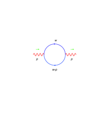
Figure 1: One-loop correction to the photon propagator.

III THE ONE-LOOP PHOTON PROPAGATOR

The one-loop correction to the photon propagator is depicted in Fig. 1. Using Feynman rules, it corresponds to the expression

$$\Pi_{\mu\nu}(p)\,=\,\int\frac{d^{3}w}{(2\,\pi)^{3}}{\it S}^{(0)}_{F}(w)e\gamma_{\mu}{\it S}^{(0)}_{F}(w-p)e\gamma_{\nu}\;,$$ (6)

which we define in terms in the left- and right-hand side projections as

$$\Pi_{\mu\nu}(p)=\Pi_{(+)\ \mu\nu}(p)+\Pi_{(-)\ \mu\nu}(p)\;,$$ (7)

where

$$\Pi_{(\pm)\ \mu\nu}(p)=\frac{\alpha}{2\pi^{2}}\int\frac{d^{3}w}{(2\,\pi)^{3}}\frac{[{\not\!w}+m_{\pm}]\gamma_{\mu}[{\not\!w-\not\!p}+m_{\pm}]\gamma_{\nu}}{[w^{2}+m_{\pm}^{2}][(w-p)^{2}+m_{\pm}^{2}]}\chi_{\pm}\;.$$

To evaluate these expressions, we propose the following decomposition:

$$\Pi_{(\pm)\ \mu\nu}(p) = \frac{\alpha}{2\pi^{2}}\Bigg{[}K_{\sigma\beta}\gamma_{\sigma}\gamma_{\mu}\gamma_{\beta}\gamma_{\nu}-K_{\sigma}\gamma_{\sigma}\gamma_{\mu}{\not\!p}\gamma_{\nu}-2m_{\pm}K_{\sigma}\delta_{\mu\sigma}\gamma_{\nu}-m_{\pm}\gamma_{\mu}{\not\!p}\gamma_{\nu}$$ (8)

$$+m_{\pm}^{2}\gamma_{\mu}\gamma_{\nu}\Bigg{]}\chi_{\pm}\;,$$

where we have written the propagator in terms of

$$K = \int d^{3}w\frac{1}{[w^{2}+m_{\pm}^{2}][(w-p)^{2}+m_{\pm}^{2}]}\;,$$

$$K_{\mu} = \int d^{3}w\frac{w_{\mu}}{[w^{2}+m_{\pm}^{2}][(w-p)^{2}+m_{\pm}^{2}]}\;,$$

$$K_{\mu\nu} = \int d^{3}w\frac{w_{\mu}w_{\nu}}{[w^{2}+m_{\pm}^{2}][(w-p)^{2}+m_{\pm}^{2}]}\;.$$ (9)

These can be evaluated straightforwardly, using standard techniques (see the Appendix for further details and also Ref. Yajaira ). Following Ref. raya , we define

$$I(p,m)=\frac{1}{p}\arctan{\frac{p}{m}}\;,$$ (10)

so that the basis integrals may be expressed as

$$K = \pi^{2}I\left(\frac{p}{2},m_{\pm}\right)\;,$$ (11)

$$K_{\mu} = \pi^{2}\frac{p_{\mu}}{2}I\left(\frac{p}{2},m_{\pm}\right)\;,$$ (12)

$$K_{\mu\nu} = \pi^{2}\delta_{\mu\nu}\bigg{[}\frac{m_{\pm}}{2}-\bigg{(}\frac{p^{2}+4m_{\pm}^{2}}{8}\bigg{)}I\left(\frac{p}{2},m_{\pm}\right)\bigg{]}$$ (13)

$$+\ \pi^{2}\frac{p_{\mu}p_{\nu}}{p^{2}}\bigg{[}\frac{m_{\pm}}{2}-\bigg{(}\frac{3p^{2}+4m_{\pm}^{2}}{8}\bigg{)}I\left(\frac{p}{2},m_{\pm}\right)\bigg{]}\;.$$

Using the results (11)-(13) into the decomposition (8) and making the replacement $m_{\pm}\to m$ we obtain the photon propagator in accordance to the results in Refs. Delbourgo ; Chaichian . This completes our calculation of the one-loop photon propagator. Next we calculate the fermion propagator at one-loop.

IV ONE-LOOP FERMION PROPAGATOR

Figure 2: One-loop correction to the fermion propagator.

The one-loop correction to the fermion propagator has been previously considered by some of us in Ref. raya , and corresponds to the diagram in Fig. 2. To calculate this correction, we write the one-loop fermion propagator as

$$S_{F}^{(1)}(p)=S_{+}^{(1)}(p)+S_{-}^{(1)}(p)\;,$$ (14)

where

$$S_{\pm}(p)=-\frac{A_{\pm}^{(1)}(p){\not\!p}+B_{\pm}^{(1)}(p)}{\left[A_{\pm}^{(1)}(p)\right]^{2}p^{2}+\left[B_{\pm}^{(1)}(p)\right]^{2}}\chi_{\pm}\;.$$ (15)

The functions $A_{\pm}^{(1)}(p)$ and $B_{\pm}^{(1)}(p)$ are thus obtained as

$$A_{\pm}^{(1)}(p) = -\frac{2\pi\alpha}{p^{2}}\int\frac{d^{3}w}{(2\pi)^{3}}{\rm Tr}\left[{\not\!p}\gamma_{\mu}S_{\pm}^{(1)}(w)\gamma_{\nu}\Delta_{\mu\nu}^{(0)}(w-p;\xi)\chi_{\pm}\right]\;,$$

$$B_{\pm}^{(1)}(p) = 2\pi\alpha\int\frac{d^{3}w}{(2\pi)^{3}}{\rm Tr}\left[\gamma_{\mu}S_{\pm}^{(1)}(w)\gamma_{\nu}\Delta_{\mu\nu}^{(0)}(w-p;\xi)\chi_{\pm}\right]\;.$$ (16)

Performing the traces, after suitable manipulations, these functions can be expressed in the form (compare against Eq (26) of Ref. raya )

$$A_{\pm}^{(1)}(p) = -\frac{\alpha\xi}{4\pi^{2}}\frac{(p^{2}\!-\!m^{2})^{2}}{p^{2}}\left[{\cal I}_{2}(p^{2},m^{2})\!-\!{\cal I}(0,m^{2}_{\pm},p^{2})\right]$$

$$+\frac{\alpha}{4\pi^{2}\theta^{2}p^{2}}\Bigg{[}(p^{2}-m^{2})^{2}{\cal I}(0,m^{2}_{\pm},p^{2})-\left[(p^{2}-m^{2})^{2}+\theta^{4}\right]{\cal I}(\theta^{2},m^{2}_{\pm},p^{2})-\theta^{2}{\cal T}(m^{2})\Bigg{]}$$

$$\mp\frac{\alpha m_{\pm}}{2\pi^{2}p^{2}}\Bigg{[}(p^{2}+m^{2}-\theta^{2}){\cal I}(\theta^{2},m^{2}_{\pm},p^{2})-(p^{2}+m^{2}){\cal I}(0,m^{2},p^{2})-{\cal T}(\theta^{2})\Bigg{]}\;,$$

$$B_{\pm}^{(1)}(p) = \frac{\alpha\xi m_{\pm}}{2\pi^{2}}{\cal I}(0,m^{2}_{\pm},p^{2})+\frac{\alpha m_{\pm}}{\pi^{2}}{\cal I}(\theta^{2},m_{\pm}^{2},p^{2})$$ (17)

$$\mp\frac{\alpha}{2\pi^{2}\theta}\Bigg{[}(p^{2}+\theta^{2}+m_{\pm}^{2}){\cal I}(\theta^{2},m_{\pm}^{2},p^{2})-(p^{2}+m_{\pm}^{2}){\cal I}(0,m^{2},p^{2})-{\cal T}(\theta^{2})\Bigg{]}\;,$$

where the master integrals are

$${\cal T}(m^{2}_{\pm})\ =\ \int d^{3}w\frac{1}{w^{2}+m^{2}_{\pm}}\;,$$

$${\cal I}(\theta^{2},m^{2}_{\pm},p^{2})\ =\ \int d^{3}w\frac{1}{[w^{2}+\theta^{2}][(p-w)^{2}+m_{\pm}^{2}]},$$

$${\cal I}_{2}(m^{2}_{\pm},p^{2})\ =\ \int d^{3}w\frac{1}{w^{4}[(p-w)^{2}+m_{\pm}^{2}]}.$$ (18)

These integrals are performed using standard techniques (see Appendix), and give

$${\cal T}(m^{2}_{\pm}) = -2\pi^{2}m_{\pm}\;,$$

$${\cal I}(\theta^{2},m^{2}_{\pm},p^{2}) = 2\pi^{2}I(p,m_{\pm}^{2}+\theta^{2})\;,$$

$${\cal I}_{2}(m^{2}_{\pm},p^{2}) = -\frac{2\pi^{2}m_{\pm}}{(p^{2}+m_{\pm}^{2})^{2}}\;.$$ (19)

Inserting the above results into the decompositions (17) and (15), we obtain the one-loop correction to the fermion propagator, in accordance with Eq. (27) of Ref. raya . This completes the one-loop correction of the two-point Green’s functions corresponding to the Lagrangian (1). Next we calculate the one-loop correction to the fermion-photon vertex.

V ONE-LOOP FERMION-PHOTON VERTEX

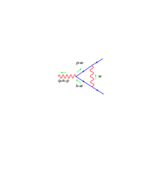
Figure 3: One-loop correction to the fermion-photon vertex.

At ${\cal O}(\alpha)$, the fermion-photon vertex is depicted in Fig. 3, and corresponds to

$$\Gamma_{\mu}(k,p)=\,\gamma_{\mu}+\,\Lambda_{\mu}\;.$$ (20)

Using the Feynman rules, $\Lambda_{\mu}$ is simply given by

$$\Lambda_{\mu}=e^{2}\int\frac{d^{3}w}{(2\,\pi)^{3}}\gamma_{\alpha}{\it S}^{(0)}_{F}(p-w)\gamma_{\mu}{\it S}^{(0)}_{F}(k-w)\gamma_{\beta}\Delta^{(0)}_{\alpha\beta}(w).$$

(21)

Given the properties of the projectors in (3), the crossed structures vanish and therefore we have only integrals with the same mass propagators ($m_{+}$ or $m_{-}$). Given this, we can write $\Lambda_{\mu}$ as

$$\Lambda_{\mu}\equiv\Lambda_{(+)\ \mu}+\Lambda_{(-)\ \mu}$$ (22)

where

$$\Lambda_{(\pm)\ \mu} = \frac{\,{\alpha}}{2\,{\pi}^{2}}\{\left[\gamma_{\sigma}{\not\!p}\,{\gamma_{\mu}}\,{\not\!k}\gamma_{\sigma}+m_{\pm}(4k_{\mu}+4p_{\mu}-{\not\!p}{\gamma_{\mu}}-{\gamma_{\mu}}{\not\!k})-m_{\pm}^{2}{\gamma_{\mu}}\right]{\it J}^{(0)}(\theta,m_{\pm})$$ (23)

$$\hskip 28.45274pt-\left[{\gamma_{\sigma}}{\not\!p}\,{\gamma_{\mu}}{\gamma_{\nu}}\gamma_{\sigma}+\gamma_{\sigma}{\gamma_{\nu}}{\gamma_{\mu}}{\not\!k}\gamma_{\sigma}-6m_{\pm}\delta_{\mu\nu}\right]{{\it J}_{\nu}^{(1)}}(\theta,m_{\pm})+{\gamma_{\sigma}}{\gamma_{\nu}}{\gamma_{\mu}}{\gamma_{\lambda}}\gamma_{\sigma}{{\it J}_{\nu\lambda}^{(2)}}(\theta,m_{\pm})$$

$$\hskip 28.45274pt+\xi[{\gamma_{\mu}}{\it K}^{(0)}(m_{\pm})-\left[{\gamma_{\nu}}{\not\!p}\,{\gamma_{\mu}}+\,{\gamma_{\mu}}{\not\!k}\,{\gamma_{\nu}}-2m_{\pm}\delta_{\mu\nu}\right]{\it J}_{\nu}^{(1)}(m_{\pm})$$

$$\hskip 28.45274pt+\left[{\gamma_{\nu}}{\not\!p}\,{\gamma_{\mu}}{\not\!k}\,{\gamma_{\lambda}}+m_{\pm}(\,{\gamma_{\nu}}{\not\!p}\,{\gamma_{\mu}}\,{\gamma_{\lambda}}+\,{\gamma_{\nu}}\,{\gamma_{\mu}}\,{\not\!k}\,{\gamma_{\lambda}})+m^{2}_{\pm}\,{\gamma_{\nu}}\,{\gamma_{\mu}}\,{\gamma_{\lambda}}\right]{{\it I}_{\nu\lambda}^{(2)}}(m_{\pm})]$$

$$\hskip 28.45274pt-{\gamma_{\mu}}[{\it K}^{(0)}(m_{\pm})-\theta^{2}{\it J}^{(0)}(\theta,m_{\pm})]-\left[{\gamma_{\nu}}{\not\!p}\,{\gamma_{\mu}}+\,{\gamma_{\mu}}{\not\!k}\,{\gamma_{\nu}}-2m_{\pm}\delta_{\mu\nu}\right]{\it J}_{\nu}^{(1)}(\theta,m_{\pm})$$

$$\hskip 28.45274pt+\left[{\gamma_{\nu}}{\not\!p}\,{\gamma_{\mu}}{\not\!k}\,{\gamma_{\lambda}}+m_{\pm}(\,{\gamma_{\nu}}{\not\!p}\,{\gamma_{\mu}}\,{\gamma_{\lambda}}+\,{\gamma_{\nu}}\,{\gamma_{\mu}}\,{\not\!k}\,{\gamma_{\lambda}})+m^{2}_{\pm}\,{\gamma_{\nu}}\,{\gamma_{\mu}}\,{\gamma_{\lambda}}\right]{{\it L}_{\nu\lambda}^{(2)}}(\theta,m_{\pm})$$

$$\hskip 28.45274pt-\theta\varepsilon_{\nu\lambda\rho}[-\left[{\gamma_{\nu}}{\not\!p}\,{\gamma_{\mu}}\,{\gamma_{\rho}}\,{\gamma_{\lambda}}+\,{\gamma_{\nu}}\,{\gamma_{\rho}}\,{\gamma_{\mu}}\,{\not\!k}\,{\gamma_{\lambda}}+m_{\pm}(\gamma_{\nu}\,{\gamma_{\rho}}\,{\gamma_{\mu}}\,{\gamma_{\lambda}}+\gamma_{\nu}\,{\gamma_{\mu}}\,{\gamma_{\rho}}\,{\gamma_{\lambda}})\right]{\it J}^{(0)}(\theta,m_{\pm})$$

$$\hskip 28.45274pt+\gamma_{\nu}\,{\gamma_{\sigma}}\,{\gamma_{\mu}}\,\gamma_{\rho}\,{\gamma_{\lambda}}{\it J}^{(1)}_{\sigma}(\theta,m_{\pm})+[{\gamma_{\nu}}{\not\!p}\,{\gamma_{\mu}}{\not\!k}\,{\gamma_{\lambda}}+m_{\pm}(\,{\gamma_{\nu}}{\not\!p}\,{\gamma_{\mu}}\,{\gamma_{\lambda}}+\,{\gamma_{\nu}}\,{\gamma_{\mu}}\,{\not\!k}\,{\gamma_{\lambda}})$$

$$\hskip 28.45274pt+m^{2}_{\pm}\,{\gamma_{\nu}}\,{\gamma_{\mu}}\,{\gamma_{\lambda}}]{{\it L}_{\rho}^{(1)}}(\theta,m_{\pm})]\}\chi_{\pm}.$$

In this expression we have introduced the basis integrals ${K^{(0)}}$, $J^{(0)}$, $J^{(1)}_{\mu}$, $J^{(2)}_{\mu\nu}$, $I^{(0)}$, $I^{(1)}_{\mu}$, $I^{(2)}_{\mu\nu}$, $L^{(1)}_{\mu}$, $L^{(2)}_{\mu\nu}$ which we define as

$${\it K}^{(0)}({m_{\pm}}) = \int\,d^{3}w\,\frac{1}{[(p-w)^{2}+m^{2}_{\pm}]\,[(k-w)^{2}+m^{2}_{\pm}]}\;,$$

$${\it J}^{(0)}(m_{\pm}) = \int\,d^{3}w\,\frac{1}{w^{2}\,[(p-w)^{2}+m^{2}_{\pm}]\,[(k-w)^{2}+m^{2}_{\pm}]}\;,$$

$${\it J}^{(0)}(\theta,m_{\pm}) = \int\,d^{3}w\,\frac{1}{[w^{2}+\theta^{2}]\,[(p-w)^{2}+m^{2}_{\pm}]\,[(k-w)^{2}+m^{2}_{\pm}]}\;,$$

$${\it J}^{(1)}_{\mu}(m_{\pm}) = \int\,d^{3}w\,\frac{w_{\mu}}{w^{2}\,[(p-w)^{2}+m^{2}_{\pm}]\,[(k-w)^{2}+m^{2}_{\pm}]}\;,$$

$${\it J}^{(1)}_{\mu}(\theta,m_{\pm}) = \int\,d^{3}w\,\frac{w_{\mu}}{[w^{2}+\theta^{2}]\,[(p-w)^{2}+m^{2}_{\pm}]\,[(k-w)^{2}+m^{2}_{\pm}]}\;,$$

$${\it J}^{(2)}_{\mu\nu}(m_{\pm}) = \int\,d^{3}w\,\frac{w_{\mu}w_{\nu}}{w^{2}\,[(p-w)^{2}+m^{2}_{\pm}]\,[(k-w)^{2}+m^{2}_{\pm}]}\;,$$

$${\it J}^{(2)}_{\mu\nu}(\theta,m_{\pm}) = \int\,d^{3}w\,\frac{w_{\mu}w_{\nu}}{[w^{2}+\theta^{2}]\,[(p-w)^{2}+m^{2}_{\pm}]\,[(k-w)^{2}+m^{2}_{\pm}]}\;,$$

$${\it I}^{(0)}(m_{\pm}) = \int\,d^{3}w\,\frac{1}{w^{4}\,[(p-w)^{2}+m^{2}_{\pm}]\,[(k-w)^{2}+m^{2}_{\pm}]}\;,$$

$${\it I}^{(1)}_{\mu}(m_{\pm}) = \int\,d^{3}w\,\frac{w_{\mu}}{w^{4}\,[(p-w)^{2}+m^{2}_{\pm}]\,[(k-w)^{2}+m^{2}_{\pm}]}\;,$$

$${\it I}^{(2)}_{\mu\nu}(m_{\pm}) = \int\,d^{3}w\,\frac{w_{\mu}w_{\nu}}{w^{4}\,[(p-w)^{2}+m^{2}_{\pm}]\,[(k-w)^{2}+m^{2}_{\pm}]}\;,$$

$${\it L}^{(1)}_{\mu}(\theta,m_{\pm}) = \int\,d^{3}w\,\frac{w_{\mu}}{w^{2}\,[w^{2}+\theta^{2}]\,[(p-w)^{2}+m^{2}_{\pm}]\,[(k-w)^{2}+m^{2}_{\pm}]}\;,$$

$${\it L}^{(2)}_{\mu\nu}(\theta,m_{\pm}) = \ \int\,d^{3}w\,\frac{w_{\mu}w_{\nu}}{w^{2}\,[w^{2}+\theta^{2}]\,[(p-w)^{2}+m^{2}_{\pm}]\,[(k-w)^{2}+m^{2}_{\pm}]}\;.$$ (24)

From this list of integrals, those which depend only on fermion masses have been calculated in Raya-Bashir and for them we just replace $m\to m_{\pm}$ to obtain the results needed in the calculation at hand. The rest correspond to two-, three- and four-point integrals that depend both on a fermion and a gauge boson mass, therefore they might be useful in theories in other space-time dimensions. We solve these in arbitrary dimensions in the Appendix. Also, it is important to mention that these results are crucial to our interest in the impact of the CS term on certain physical observables related to the Lagrangian (1).

These results along with the decomposition proposed in Eq. (23) complete the calculation of the one-loop correction of the fermion-photon vertex. We summarize our findings in the next section.

VI Summary and conclusions

We have derived the one-loop correction to the photon propagator, fermion propagator and the fermion-photon vertex in Maxwell-Chern-Simons in QED₃. In doing so, we have proposed a basis of master integrals to expand said Green functions, some of them new in literature. Due to the potential applications of two- and three-point Green functions with a massive gauge boson in physical processes in several frameworks of particle and condensed matter physics, we evaluated these new integrals in arbitrary space-time dimensions. The basis expansion contains the ordinary expansion of QED₃ as the particular case of our findings in the parity preserving limit Raya-Bashir , which is achieved when both the CS term and the Haldane mass are taken to zero. Massless theory for both fermions and photons bashir follows as well. Green functions we have obtained will help us make progress in certain physical applications in the near future. Particularly, we are interested in the radiative generation of fermion masses by the CS term and its impact in several physical observables. This project is in progress and the results will be presented elsewhere.

Appendix

In this Appendix we provide details in the calculations for three sets of master integrals: for the one-loop photon propagator described in (13), the one-loop fermion propagator, Eq. (18), and for the one-loop vertex described in (24). Let us begin with the $K$-type master integrals.

1. $K$

We begin solving $K$. Using

$$\frac{1}{ab}=\int_{0}^{1}\frac{dx}{[xa+(1-x)b]^{2}}\;,$$ (25)

we can write

$$K = \int_{0}^{1}dx\int d^{3}w\frac{1}{\bigg{[}x[(w-p)^{2}+m^{2}_{\pm}]+(1-x)(w^{2}+m^{2}_{\pm})\bigg{]}^{2}}\;.$$ (26)

The denominator in the above expression can be written as $w^{2}-2xw\cdot p+xp^{2}+m^{2}_{\pm}$, which after the change of variables $w^{\prime}=w-px$, allows us to write

$$K=\int_{0}^{1}dx\int d^{3}w^{\prime}\frac{1}{[(w^{\prime})^{2}+p^{2}x(1-x)+m^{2}_{\pm}]^{2}}\;.$$ (27)

This integral has the following form:

$$\int\frac{d^{D}w}{(w^{2}-s)^{n}}=(-1)^{n}\pi^{D/2}\frac{\Gamma\big{(}n-\frac{D}{2}\big{)}}{\Gamma(n)}\frac{1}{s^{n-D/2}}\;.$$ (28)

In our case, we take $D=3$, $n=2$ and $s=-p^{2}x(1-x)-m^{2}_{\pm}$, and then

$$K=\pi^{3/2}\Gamma\bigg{(}\frac{1}{2}\bigg{)}\int_{0}^{1}dx[-p^{2}x(1-x)-m^{2}_{\pm}]^{-1/2}=\frac{2\pi^{2}}{p}\arctan\bigg{(}\frac{p}{2m_{\pm}}\bigg{)}\;.$$ (29)

2. $K_{\mu}$

Now, we calculate $K_{\mu}$. This integral depends only of $p_{\mu}$, thus we can write

$$K_{\mu}\equiv cp_{\mu}\;.$$ (30)

We find $c$ multiplying with $p_{\mu}$ on both sides

$$cp^{2}=\int d^{3}w\frac{w\cdot p}{(w^{2}+m^{2}_{\pm})[(w-p)^{2}+m^{2}_{\pm}]}\;.$$ (31)

Using $w\cdot p=w^{2}+p^{2}-(w-p)^{2}$, we have

$$c = \frac{1}{2}K\;.$$ (32)

3. ${K_{\mu\nu}}$

Finally, we solve $K_{\mu\nu}$. In its most general form, it depends only on $p_{\mu}p_{\nu}$ and $\delta_{\mu\nu}$,

$$K_{\mu\nu}\equiv a\bigg{[}\frac{p_{\mu}p_{\nu}}{p^{2}}+\frac{1}{3}\delta_{\mu\nu}\bigg{]}-b\delta_{\mu\nu}\;,$$ (33)

which is symmetrical under the exchange of $\mu$ and $\nu$. After simplifying, we find that

$$a=\frac{1}{4}\int d^{3}w\frac{1}{w^{2}+m^{2}_{\pm}}-\frac{3p^{2}+4m^{2}_{\pm}}{8}K\;,$$ (34)

and

$$b=\frac{1}{3}\int\frac{d^{3}w}{(w-p)^{2}+m^{2}_{\pm}}+\frac{m^{2}_{\pm}}{3}K\;,$$ (35)

where the tadpole integrals [see Eq. (37) below] are

$${\cal T}(m_{\pm}^{2})\ =\ \int d^{3}w\frac{1}{w^{2}+m^{2}_{\pm}}=\int\frac{d^{3}w}{(w-p)^{2}+m^{2}_{\pm}}=-2\pi^{2}m_{\pm}\;.$$ (36)

Next, we provide details of the calculation of the integrals in Eq. (18).

4. ${\cal T}(m_{\pm}^{2})$

The integral

$${\cal T}(m_{\pm}^{2})=\int d^{3}w\frac{1}{w^{2}+m_{\pm}^{2}}$$ (37)

can be evaluated directly from Eq. (28) with $n=1$, $D=3$ and $s=-m_{\pm}^{2}$. It yields

$${\cal T}(m_{\pm}^{2})=-2\pi^{2}m_{\pm}.$$ (38)

5. ${\cal I}(\theta^{2},m_{\pm}^{2},p^{2})$

Let us evaluate

$${\cal I}(\theta^{2},m_{\pm}^{2},p^{2})=\int d^{3}w\frac{1}{[w^{2}+\theta^{2}][(p-w)^{2}+m_{\pm}^{2}]}.$$ (39)

Using Feynman parametrization, and after the appropriate change of variables, we can write

$${\cal I}(\theta^{2},m_{\pm}^{2},p^{2}) = \int_{0}^{1}\int d^{3}w^{\prime}\frac{1}{[(w^{\prime})^{2}+x(1-x)p^{2}+m_{\pm}^{2}x+\theta^{2}(1-x)]^{2}}$$ (40)

$$= \pi^{2}\int_{0}^{1}dx(x(1-x)p^{2}+m_{\pm}^{2}x+\theta^{2}(1-x))^{-\frac{1}{2}}$$

$$= 2\pi^{2}I(p,m_{\pm}^{2}+\theta^{2})\;.$$

6. ${\cal I}_{2}(m_{\pm}^{2},p^{2})$

In order to evaluate

$${\cal I}_{2}(m_{\pm}^{2},p^{2})=\int d^{3}w\frac{1}{w^{4}[(p-w)^{2}+m_{\pm}^{2}]}\;,$$ (41)

we introduce the auxiliary integral

$${\cal I}_{\mu}(m_{\pm}^{2},p^{2})=\int d^{3}w\frac{w_{\mu}}{w^{4}[(p-w)^{2}+m_{\pm}^{2}]}\;,$$ (42)

such that

$$p_{\mu}{\cal I}_{\mu}(m_{\pm}^{2},p^{2})=\frac{1}{2}((p^{2}+m_{\pm}^{2}){\cal I}_{2}(m_{\pm}^{2},p^{2})+{\cal I}(0,m_{\pm}^{2},p^{2}))\;.$$ (43)

Using the identity

$$\frac{1}{A^{n}B^{p}}=\frac{\Gamma(n+p)}{\Gamma(n)\Gamma(p)}\int_{0}^{1}dxx^{n-1}(1-x)^{p-1}\frac{1}{[xA+(1-x)B]^{n+p}}\;,$$ (44)

with $n=1$, $p=2$, followed by the shift $w^{\prime}=w-px$, we can write

$${\cal I}_{\mu}(m_{\pm}^{2},p^{2})=2\int_{0}^{1}dx(1-x)\int d^{3}w^{\prime}\frac{p_{\mu}x}{[(w^{\prime})^{2}+p^{2}x(1-x)+m_{\pm}^{2}x]^{3}}\;,$$ (45)

performing the $w^{\prime}$ integration,

$${\cal I}_{\mu}(m_{\pm}^{2},p^{2})=\frac{\pi^{2}}{2}p_{\mu}\int_{0}^{1}dx(x^{-\frac{1}{2}}-x^{\frac{1}{2}})[p^{2}(1-x)+m_{\pm}^{2}]^{-\frac{3}{2}}\;,$$ (46)

and the remaining integration yields

$${\cal I}_{\mu}(m_{\pm}^{2},p^{2}) = \frac{\pi^{2}}{p^{2}}p_{\mu}\left[-\frac{m_{\pm}}{p^{2}+m_{\pm}^{2}}+I(p,m_{\pm})\right]\;.$$ (47)

Thus

$${\cal I}_{2}(m_{\pm}^{2},p^{2})=\frac{2p_{\mu}{\cal I}_{\mu}(m_{\pm}^{2},p^{2})-{\cal I}(0,m_{\pm}^{2},p^{2})}{p^{2}+m_{\pm}^{2}}=-\frac{2\pi^{2}m_{\pm}}{(p^{2}+m_{\pm}^{2})^{2}}\;.$$ (48)

Next, we will give the results for the new integrals that are described in (24).

7. $J^{(0)}(\theta,m_{\pm})$

We begin solving $J^{(0)}(\theta,m_{\pm})$. For this purpose, we consider the following integral in Minkowski space:

$${\cal J}^{(0)}_{\nu_{1},\nu_{2},\nu_{3}}(\theta,m_{\pm})=\int_{M}d^{D}w\frac{1}{[(p-w)^{2}-m_{\pm}^{2}]^{\nu_{1}}[w^{2}-\theta^{2}]^{\nu_{2}}[(k-w)^{2}-m_{\pm}^{2}]^{\nu_{3}}}\;.$$ (49)

Using Schwinger parametrization

$$\frac{1}{[A_{1}+A_{2}]^{\nu}}=\frac{1}{2\pi i}\int_{-i\infty}^{i\infty}d\zeta A_{1}^{\zeta}A_{2}^{-\nu-\zeta}\frac{\Gamma(-\zeta)\Gamma(\nu+\zeta)}{\Gamma(\nu)}$$ (50)

to each of the factors in the denominator, the Mellin-Barnes representation for ${\cal J}^{(0)}_{\nu_{1},\nu_{2},\nu_{3}}(\theta,m_{\pm})$ becomes

$${\cal J}^{(0)}_{\nu_{1},\nu_{2},\nu_{3}}(\theta,m_{\pm}) \equiv \frac{1}{(2\pi i)^{3}\Gamma(\nu_{1})\Gamma(\nu_{2})\Gamma(\nu_{3})}\int_{-i\infty}^{+i\infty}\int_{-i\infty}^{+i\infty}\int_{-i\infty}^{+i\infty}d\lambda_{3}d\lambda_{34}d\lambda_{5}(-m^{2})^{\lambda_{34}}(-\theta^{2})^{\lambda_{5}}$$ (51)

$$\times\Gamma(-\lambda_{3})\Gamma(-\lambda_{34}+\lambda_{3})\Gamma(-\lambda_{5})\Gamma(\lambda_{3}+\nu_{1})\Gamma(\lambda_{34}-\lambda_{3}+\nu_{3})\Gamma(\lambda_{5}+\nu_{2})$$

$$\times{\cal J}^{(0)}_{\nu_{1}+\lambda_{3},\nu_{2}+\lambda_{5},\nu_{3}+\lambda_{34}-\lambda_{3}}(0,0)\;,$$

where we have used the notation $\lambda_{34}=\lambda_{3}+\lambda_{4}$ and $d\lambda_{4}=d\lambda_{34}\;,$ and where $J^{(0)}_{\nu_{1}+\lambda_{3},\nu_{2}+\lambda_{5},\nu_{3}+\lambda_{34}-\lambda_{3}}(0,0)$ has been calculated in Ref. davydychev . Replacing these results and simplifying, we obtain the following expression in terms of five integrals to evaluate

$${\cal J}^{(0)}_{\nu_{1},\nu_{2},\nu_{3}}(\theta,m_{\pm}) = \frac{(i)^{D}}{\prod_{i=1}^{3}\Gamma(\nu_{i})}\frac{(k^{2})^{D/2-\nu_{123}}}{(2\pi i)^{5}}\int\int\int\int\int_{-i\infty}^{+i\infty}d\lambda_{1}d\lambda_{2}d\lambda_{3}d\lambda_{34}d\lambda_{5}\Gamma(-\lambda_{1})$$ (52)

$$\times\Gamma(-\lambda_{2})\Gamma(-\lambda_{3})\Gamma(\lambda_{3}-\lambda_{34})\Gamma(-\lambda_{5})\bigg{(}\frac{p^{2}}{k^{2}}\bigg{)}^{\lambda_{1}}\bigg{(}\frac{q^{2}}{k^{2}}\bigg{)}^{\lambda_{2}}\bigg{(}-\frac{m^{2}}{k^{2}}\bigg{)}^{\lambda_{34}}\bigg{(}-\frac{\theta^{2}}{k^{2}}\bigg{)}^{\lambda_{5}}$$

$$\times\frac{\Gamma\big{(}\lambda_{12}+\lambda_{34}+\nu_{123}+\lambda_{5}-\frac{D}{2}\big{)}}{\Gamma(D-\nu_{123}-\lambda_{34}-\lambda_{5})}\Gamma(\lambda_{123}+\nu_{1})\Gamma\bigg{(}-\lambda_{13}-\nu_{12}-\lambda_{5}+\frac{D}{2}\bigg{)}$$

$$\times\Gamma\bigg{(}-\lambda_{2}-\lambda_{34}-\nu_{13}+\frac{D}{2}\bigg{)}\;.$$

We perform one integration at a time. First we integrate over $\lambda_{3}$, defining

$$I_{\lambda_{3}}=\frac{1}{2\pi i}\int_{-i\infty}^{+i\infty}d\lambda_{3}\Gamma(-\lambda_{3})\Gamma(\lambda_{3}-\lambda_{34})\Gamma(\lambda_{123}+\nu_{1})\Gamma\bigg{(}-\lambda_{13}-\nu_{12}-\lambda_{5}+\frac{D}{2}\bigg{)}\;.$$ (53)

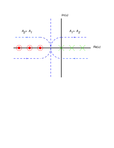
Figure 4: Mellin-Barnes contour of integration which separates the poles of $\Gamma(\ldots+u)$ from those of $\Gamma(\ldots-u)$. We close the contour to the left or to the right, choosing one of the two series of poles. $A_{1}$ and $A_{2}$ represent the arguments in the sum which are given a Schwinger representation (50).

Using the Barnes lemma

$$\frac{1}{2\pi i}\int_{-i\infty}^{+i\infty}ds\Gamma(a+s)\Gamma(b+s)\Gamma(c-s)\Gamma(d-s)=\frac{\Gamma(a+c)\Gamma(b+c)\Gamma(a+d)\Gamma(b+d)}{\Gamma(a+b+c+d)}\;,$$ (54)

with $a=-\lambda_{34}\;,b=\nu_{1}+\lambda_{12}\;,c=0\;,d=\frac{D}{2}-\nu_{12}-\lambda_{1}-\lambda_{5}\;,$ we find that

$$I_{\lambda_{3}} = \frac{\Gamma(-\lambda_{34})\Gamma(\nu_{1}+\lambda_{12})\Gamma\big{(}\lambda_{2}-\nu_{2}-\lambda_{5}+\frac{D}{2}\big{)}}{\Gamma\big{(}\lambda_{2}-\lambda_{34}-\nu_{2}-\lambda_{5}+\frac{D}{2}\big{)}}\Gamma\big{(}-\lambda_{1}-\lambda_{34}-\lambda_{5}-\nu_{12}+\frac{D}{2}\big{)}\;.$$

Then, after integrating over $\lambda_{3}$, Eq. (52) becomes

$${\cal J}^{(0)}_{\nu_{1},\nu_{2},\nu_{3}}(\theta,m_{\pm}) = \frac{(i)^{D}}{\prod_{i=1}^{3}\Gamma(\nu_{i})}\frac{(k^{2})^{D/2-\nu_{123}}}{(2\pi i)^{4}}\int\int\int\int_{-i\infty}^{+i\infty}d\lambda_{1}d\lambda_{2}d\lambda_{34}d\lambda_{5}\Gamma(-\lambda_{1})\Gamma(-\lambda_{2})$$ (55)

$$\times\Gamma(-\lambda_{5})\bigg{(}\frac{p^{2}}{k^{2}}\bigg{)}^{\lambda_{1}}\bigg{(}\frac{q^{2}}{k^{2}}\bigg{)}^{\lambda_{2}}\bigg{(}-\frac{m^{2}}{k^{2}}\bigg{)}^{\lambda_{34}}\bigg{(}-\frac{\theta^{2}}{k^{2}}\bigg{)}^{\lambda_{5}}$$

$$\times\frac{\Gamma\big{(}\lambda_{12}+\lambda_{34}+\nu_{123}+\lambda_{5}-\frac{D}{2}\big{)}\Gamma\big{(}-\lambda_{2}-\lambda_{34}-\nu_{13}+\frac{D}{2}\big{)}}{\Gamma(D-\nu_{123}-\lambda_{34}-\lambda_{5})}$$

$$\times\frac{\Gamma(-\lambda_{34})\Gamma(\nu_{1}+\lambda_{2})\Gamma\big{(}-\lambda_{1}-\lambda_{34}-\lambda_{5}-\nu_{12}+\frac{D}{2}\big{)}}{\Gamma\big{(}\lambda_{2}-\lambda_{34}-\nu_{2}-\lambda_{5}+\frac{D}{2}\big{)}}$$

$$\times\Gamma\big{(}\lambda_{2}-\nu_{2}-\lambda_{5}+\frac{D}{2}\big{)}\;.$$

One particular limit of our interest is $\theta\to 0$. We integrate over $\lambda_{5}$ first and call $I_{\lambda_{5}}$ the relevant term in the above multidimensional integration. Therefore, a wise selection of the position of the poles according to the possible closure of the contour of integration in Fig. 4 must be done in order to avoid unnecessary analytic continuation. We close the contour to the left, such that $|-\theta^{2}/k^{2}|>1$. Then, the poles are due to $\Gamma(\lambda_{12}+\lambda_{34}+\nu_{123}-\frac{D}{2}+\lambda_{5})$ alone, and are located at $\lambda_{5}=-\lambda_{12}-\lambda_{34}-\nu_{123}+\frac{D}{2}-n\;.$ Therefore

$$I_{\lambda_{5}} = 2\pi i\sum_{n=0}^{\infty}\frac{(-1)^{n}}{n!}\bigg{(}-\frac{\theta^{2}}{k^{2}}\bigg{)}^{D/2-\lambda_{12}-\lambda_{34}-\nu_{123}-n}\frac{\Gamma(\lambda_{2}+\nu_{3}+n)\Gamma\bigg{(}\lambda_{12}+\lambda_{34}+\nu_{123}-\frac{D}{2}+n\bigg{)}}{\Gamma\big{(}\frac{D}{2}+\lambda_{12}+n\big{)}\Gamma(2\lambda_{2}+\lambda_{1}+\nu_{13}+n)}\;.$$

Hence, we can write

$${\cal J}^{(0)}_{\nu_{1},\nu_{2},\nu_{3}}(\theta,m_{\pm}) = \frac{(i)^{D}}{\prod_{i=1}^{3}\Gamma(\nu_{i})}\frac{(k^{2})^{D/2-\nu_{123}}}{(2\pi i)^{3}}\sum_{n=0}^{\infty}\frac{(-1)^{n}}{n!}\int_{-i\infty}^{+i\infty}\int_{-i\infty}^{+i\infty}\int_{-i\infty}^{+i\infty}d\lambda_{1}d\lambda_{2}d\lambda_{34}\Gamma(-\lambda_{1})$$ (56)

$$\times\Gamma(-\lambda_{2})\Gamma(-\lambda_{34})\frac{\Gamma\big{(}\lambda_{2}+\nu_{3}+n\big{)}\Gamma(\lambda_{12}+\nu_{1})\Gamma\big{(}\lambda_{12}+\lambda_{34}+\nu_{123}-\frac{D}{2}+n\big{)}}{\Gamma\big{(}\frac{D}{2}+n+\lambda_{12}\big{)}\Gamma(n+\nu_{13}+\lambda_{1}+2\lambda_{2})}$$

$$\times\Gamma(-\lambda_{2}-\lambda_{34}-\nu_{13}+\frac{D}{2})\bigg{(}\frac{p^{2}}{k^{2}}\bigg{)}^{\lambda_{1}}\bigg{(}\frac{q^{2}}{k^{2}}\bigg{)}^{\lambda_{2}}\bigg{(}-\frac{m^{2}}{k^{2}}\bigg{)}^{\lambda_{34}}$$

$$\times\bigg{(}-\frac{\theta^{2}}{k^{2}}\bigg{)}^{D/2-\lambda_{12}-\lambda_{34}-\nu_{123}-n}\;.$$

Next, we integrate with respect to $\lambda_{34}$ closing the contour in Fig. 4 to the left, where $|-m^{2}/k^{2}|>1$. Naming $I_{\lambda_{34}}$ the relevant term, we have that

$$I_{\lambda_{34}} = \int_{-i\infty}^{+i\infty}d\lambda_{34}\bigg{(}-\frac{m^{2}}{k^{2}}\bigg{)}^{\lambda_{34}}\bigg{(}-\frac{\theta^{2}}{k^{2}}\bigg{)}^{D/2-\lambda_{12}-\lambda_{34}-\nu_{123}-n}\Gamma(-\lambda_{34})\Gamma\bigg{(}-\lambda_{2}-\lambda_{34}-\nu_{13}+\frac{D}{2}\bigg{)}$$

$$\times\Gamma\bigg{(}\lambda_{12}+\lambda_{34}+\nu_{123}-\frac{D}{2}+n\bigg{)}\;.$$

The poles in $I_{\lambda_{34}}$ are due to $\Gamma(\lambda_{12}+\lambda_{34}+\nu_{123}-\frac{D}{2}+n)$, and are located at $\lambda_{34}=-\lambda_{12}-\nu_{123}+D/2-n$. Thus

$$I_{\lambda_{34}} = 2\pi i\sum_{l=0}^{\infty}\frac{(-1)^{l}}{l!}\bigg{(}-\frac{\theta^{2}}{k^{2}}\bigg{)}^{l}\bigg{(}-\frac{m^{2}}{k^{2}}\bigg{)}^{-\lambda_{12}-\nu_{123}+D/2-n-l}\Gamma(\lambda_{1}+n+l+\nu_{2})$$

$$\times\Gamma\bigg{(}\lambda_{12}+l+\nu_{123}-\frac{D}{2}+n\bigg{)}\;.$$

Then we can write

$${\cal J}^{(0)}_{\nu_{1},\nu_{2},\nu_{3}}(\theta,m_{\pm}) = \frac{(i)^{D}(k^{2})^{D/2-\nu_{123}}}{\prod_{i=1}^{3}\Gamma(\nu_{i})(2\pi i)^{2}}\sum_{n,l=0}^{\infty}\frac{(-1)^{n}}{n!}\frac{(-1)^{l}}{l!}\bigg{(}-\frac{\theta^{2}}{k^{2}}\bigg{)}^{l}\int_{-i\infty}^{+i\infty}\int_{-i\infty}^{+i\infty}d\lambda_{1}d\lambda_{2}\Gamma(-\lambda_{1})$$ (57)

$$\times\Gamma(-\lambda_{2})\bigg{(}\frac{p^{2}}{k^{2}}\bigg{)}^{\lambda_{1}}\bigg{(}-\frac{m^{2}}{k^{2}}\bigg{)}^{\lambda_{12}-\nu_{123}+D/2-n-l}\bigg{(}\frac{q^{2}}{k^{2}}\bigg{)}^{\lambda_{2}}\Gamma(\lambda_{12}+\nu_{1})\Gamma(\lambda_{2}+\nu_{3}+n)$$

$$\times\Gamma\bigg{(}\lambda_{12}+\nu_{123}-\frac{D}{2}+n+l\bigg{)}\frac{\Gamma(\lambda_{1}+\nu_{2}+n+l)}{\Gamma\big{(}\lambda_{12}+\frac{D}{2}+n\big{)}\Gamma(2\lambda_{2}+\lambda_{1}+n+\nu_{13})}\;.$$

Now we integrate with respect to $\lambda_{2}$, but now closing the contour in Fig. 4 to the right, such that $|q^{2}/k^{2}|<1$. Calling $I_{\lambda_{2}}$ to the corresponding contribution, we have

$$I_{\lambda_{2}} = \int_{-i\infty}^{+i\infty}d\lambda_{2}\bigg{(}\frac{q^{2}}{k^{2}}\bigg{)}^{\lambda_{2}}\bigg{(}-\frac{m^{2}}{k^{2}}\bigg{)}^{-\lambda_{12}-\nu_{123}+D/2-n-l}\Gamma(-\lambda_{2})\Gamma(\lambda_{12}+\nu_{1})\Gamma(\lambda_{2}+\nu_{3}+n)$$

$$\frac{\Gamma\big{(}\lambda_{12}+n+l+\nu_{123}-\frac{D}{2}\big{)}}{\Gamma\big{(}\lambda_{12}+\frac{D}{2}+n\big{)}\Gamma(2\lambda_{2}+\lambda_{1}+n+\nu_{13})}\;.$$

There are poles in this expression are due to $\Gamma(-\lambda_{2})$ and are located at $\lambda_{2}=j$. Therefore

$$I_{\lambda_{2}} = 2\pi i\sum_{j=0}^{\infty}\frac{(-1)^{j}}{j!}\bigg{(}\frac{q^{2}}{k^{2}}\bigg{)}^{j}\bigg{(}-\frac{m^{2}}{k^{2}}\bigg{)}^{-\lambda_{1}-j-\nu_{123}+D/2-n-l}\Gamma(\lambda_{1}+\nu_{1}+j)\Gamma(n+j+\nu_{3})$$

$$\times\frac{\Gamma\big{(}\lambda_{1}+n+l+j+\nu_{123}-\frac{D}{2}\big{)}}{\Gamma\big{(}\lambda_{1}+n+j+\frac{D}{2}\big{)}\Gamma(\lambda_{1}+n+2j+\nu_{13})}\;,$$

and thus

$${\cal J}^{(0)}_{\nu_{1},\nu_{2},\nu_{3}}(\theta,m_{\pm}) = \frac{(i)^{D}(k^{2})^{D/2-\nu_{123}}}{\prod_{i=1}^{3}\Gamma(\nu_{i})2\pi i}\sum_{n,l,j=0}^{\infty}\frac{(-1)^{n}}{n!}\frac{(-1)^{l}}{l!}\frac{(-1)^{j}}{j!}\bigg{(}-\frac{\theta^{2}}{k^{2}}\bigg{)}^{l}\bigg{(}\frac{q^{2}}{k^{2}}\bigg{)}^{j}\Gamma(n+j+\nu_{3})$$ (58)

$$\times\int_{-i\infty}^{+i\infty}d\lambda_{1}\Gamma(-\lambda_{1})\bigg{(}\frac{p^{2}}{k^{2}}\bigg{)}^{\lambda_{1}}\bigg{(}-\frac{m^{2}}{k^{2}}\bigg{)}^{-\lambda_{1}-\nu_{123}+D/2-n-l-j}\Gamma(\lambda_{1}+n+l+\nu_{2})$$

$$\times\Gamma(\lambda_{1}+j+\nu_{1})\frac{\Gamma\big{(}\lambda_{1}+j+\nu_{123}-\frac{D}{2}+n+l\big{)}}{\Gamma\big{(}\lambda_{1}+n+j+\frac{D}{2}\big{)}\Gamma(\lambda_{1}+n+2j+\nu_{13})}\;.$$

Finally, we integrate with respect to $\lambda_{1}$ closing the contour to the right, such that $|p^{2}/k^{2}|<1$, and observing that the poles of the expression are due to $\Gamma(-\lambda_{1})$ and they are located at $\lambda_{1}=s$, we find

$${\cal J}^{(0)}_{\nu_{1},\nu_{2},\nu_{3}}(\theta,m_{\pm}) = \frac{(i)^{D}(-m^{2})^{D/2-\nu_{123}}}{\prod_{i=1}^{3}\Gamma(\nu_{i})}\sum_{n,l,j,s=0}^{\infty}\frac{(-1)^{n}}{n!}\frac{(-1)^{l}}{l!}\frac{(-1)^{j}}{j!}\frac{(-1)^{s}}{s!}\bigg{(}-\frac{k^{2}}{m^{2}}\bigg{)}^{n}\bigg{(}\frac{\theta^{2}}{m^{2}}\bigg{)}^{l}$$ (59)

$$\times\bigg{(}-\frac{q^{2}}{m^{2}}\bigg{)}^{j}\bigg{(}-\frac{p^{2}}{m^{2}}\bigg{)}^{s}\Gamma(\nu_{3}+n+j)\Gamma(\nu_{2}+n+l+s)\Gamma(\nu_{1}+j+s)$$

$$\times\frac{\Gamma\big{(}\nu_{123}-\frac{D}{2}+n+l+j+s\big{)}}{\Gamma\big{(}\frac{D}{2}+n+j+s\big{)}\Gamma(\nu_{13}+n+2j+s)}\;.$$

Changing to Pochammer symbols according to

$$\Gamma(\nu_{3}+n+j) = (\nu_{3};n+j)\Gamma(\nu_{3})\;,$$

$$\Gamma(\nu_{2}+n+l+s) = (\nu_{2};n+l+s)\Gamma(\nu_{2})\;,$$

$$\Gamma(\nu_{1}+j+s) = (\nu_{1};j+s)\Gamma(\nu_{1})\;,$$

$$\Gamma\bigg{(}\nu_{123}-\frac{D}{2}+n+l+j+s\bigg{)} = \bigg{(}\nu_{123}-\frac{D}{2};n+l+j+s\bigg{)}\Gamma\bigg{(}\nu_{123}-\frac{D}{2}\bigg{)}\;,$$

$$\Gamma(\nu_{13}+n+2j+s) = (\nu_{13};n+2j+s)\Gamma(\nu_{13})\;,$$

$$\Gamma\bigg{(}\frac{D}{2}+n+j+s\bigg{)} = \bigg{(}\frac{D}{2};n+j+s\bigg{)}\Gamma\bigg{(}\frac{D}{2}\bigg{)}\;,$$

we reach at the expression

$${\cal J}^{(0)}_{\nu_{1},\nu_{2},\nu_{3}}(\theta,m_{\pm}) = (i)^{D}(-m^{2})^{D/2-\nu_{123}}\frac{\Gamma\big{(}\nu_{123}-\frac{D}{2}\big{)}}{\Gamma\big{(}\frac{D}{2}\big{)}\Gamma(\nu_{123})}\sum_{n,l,j,s=0}^{\infty}\frac{(-1)^{n+l+j+s}}{n!l!j!s!}\bigg{(}-\frac{k^{2}}{m^{2}}\bigg{)}^{n}\bigg{(}\frac{\theta^{2}}{m^{2}}\bigg{)}^{l}$$ (60)

$$\times\bigg{(}-\frac{q^{2}}{m^{2}}\bigg{)}^{j}\bigg{(}-\frac{p^{2}}{m^{2}}\bigg{)}^{s}\frac{\big{(}\nu_{123}-\frac{D}{2};n+l+s+j\big{)}(\nu_{2};n+l+s)(\nu_{3};n+j)}{\big{(}\frac{D}{2};n+j+s\big{)}(\nu_{13};n+2j+s)}$$

$$\times(\nu_{1};j+s)\;,$$

or, equivalently

$${\cal J}^{(0)}_{\nu_{1},\nu_{2},\nu_{3}}(\theta,m_{\pm}) =$$ (63)

$$(i)^{D}(-m^{2})^{D/2-\nu_{123}}\frac{\Gamma\big{(}\nu_{123}-\frac{D}{2}\big{)}}{\Gamma\big{(}\frac{D}{2}\big{)}\Gamma(\nu_{123})}\Upsilon_{3}\left[\begin{array}[]{c}\nu_{123}-\frac{D}{2},\nu_{2},\nu_{3},\nu_{1}\\ \frac{D}{2};\nu_{13}\end{array}\Bigg{|}\frac{k^{2}}{m^{2}},\frac{\theta^{2}}{m^{2}},\frac{q^{2}}{m^{2}},\frac{p^{2}}{m^{2}}\right]\;,$$

where $\Upsilon_{3}\left[\begin{array}[]{c}a_{1},a_{2},a_{3},a_{4}\\ b_{1};b_{2}\end{array}\Bigg{|}x_{1},x_{2},x_{3},x_{4}\right]$ is the generalized Lauricella function of 4 variables. This is the general expression in arbitrary space-time dimensions. In our particular case, we take $\nu_{1}=\nu_{2}=\nu_{3}=1$ and $D=3$, and Wick rotates to Euclidean space. We hence obtain

$$J^{(0)}(\theta,m_{\pm}) = (m^{2})^{-3/2}\frac{\Gamma\big{(}3-\frac{3}{2}\big{)}}{\Gamma\big{(}\frac{3}{2}\big{)}\Gamma(3)}\sum_{n,l,j,s=0}^{\infty}\frac{(-1)^{n+l+j+s}}{n!l!j!s!}\bigg{(}\frac{k^{2}}{m^{2}}\bigg{)}^{n}\bigg{(}\frac{\theta^{2}}{m^{2}}\bigg{)}^{l}\bigg{(}\frac{q^{2}}{m^{2}}\bigg{)}^{j}\bigg{(}\frac{p^{2}}{m^{2}}\bigg{)}^{s}$$ (64)

$$\times\frac{\big{(}3-\frac{3}{2};n+l+s+j\big{)}(1;n+l+s)(1;n+j)(1;j+s)}{\big{(}\frac{3}{2};n+j+s\big{)}(2;n+2j+s)}\;,$$

or

$$J^{(0)}(\theta,m_{\pm}) = (m^{2})^{-3/2}\Upsilon_{3}\left[\begin{array}[]{c}\frac{3}{2},1,1,1\\ \frac{3}{2};2\end{array}\Bigg{|}\frac{k^{2}}{m^{2}},\frac{\theta^{2}}{m^{2}},\frac{q^{2}}{m^{2}},\frac{p^{2}}{m^{2}}\right]\;.$$ (67)

This completes the calculation of $J^{(0)}(\theta,m_{\pm})$. Next we check some particular limits.

First we consider $\theta^{2}=m^{2}$. Then

$$J^{(0)}(m_{\pm}) = (m^{2})^{-3/2}\sum_{n,j,s=0}^{\infty}\frac{(-1)^{n+j+s}}{n!j!s!}\bigg{(}\frac{k^{2}}{m^{2}}\bigg{)}^{n}\bigg{(}\frac{q^{2}}{m^{2}}\bigg{)}^{j}\bigg{(}\frac{p^{2}}{m^{2}}\bigg{)}^{s}\frac{\Gamma(s+j+1)\Gamma(n+s+1)}{\Gamma(2n+2j+2s+3)}\times$$ (69)

$$\Gamma(n+j+1)\Gamma\bigg{(}n+j+s+\frac{3}{2}\bigg{)}\;,$$

that can be written as

$$J^{(0)}(m_{\pm}) = \frac{\sqrt{\pi}}{4}(m^{2})^{-3/2}\Phi_{3}\left[\begin{array}[]{c}\frac{3}{2},1,1,1\\ 3\end{array}\Bigg{|}\frac{k^{2}}{m^{2}},\frac{q^{2}}{m^{2}},\frac{p^{2}}{m^{2}}\right]\;,$$ (72)

where $\Phi_{3}\left[\begin{array}[]{c}a_{1},a_{2},a_{3},a_{4}\\ b_{1}\end{array}\Bigg{|}x_{1},x_{2},x_{3}\right]$ is the generalized Lauricella function of three variables. This expression coincides with the Eq. (37) obtained in Ref. davydychev where, in our case, $\nu_{1}=\nu_{2}=\nu_{3}=1$ and $\nu_{1}\rightarrow\rho$, $\nu_{2}\rightarrow\mu$, $\nu_{3}\rightarrow\nu$.

Another limit of interest is when $\theta=0$. This limit is achieved by returning to Eq. (52), where we take directly $\theta=0$ and integrate using the Barnes theorem and integrating in accordance with above reasoning. Then,

$$J^{(0)}(m_{\pm}) = (m^{2})^{-3/2}\sum_{n,s,j=0}^{\infty}\frac{(-1)^{n+s+j}}{n!s!j!}\bigg{(}\frac{k^{2}}{m^{2}}\bigg{)}^{n}\bigg{(}\frac{p^{2}}{m^{2}}\bigg{)}^{s}\bigg{(}\frac{q^{2}}{m^{2}}\bigg{)}^{j}\Gamma(n+j+1)$$ (74)

$$\times\Gamma\bigg{(}n+s+j+\frac{3}{2}\bigg{)}\Gamma\bigg{(}j+\frac{1}{2}\bigg{)}\frac{\Gamma(s+j+1)\Gamma(n+s+1)}{\Gamma\big{(}n+s+j+\frac{3}{2}\big{)}\Gamma(n+s+2j+2)}$$

or

$$J^{(0)}(m_{\pm}) = \sqrt{\pi}(m^{2})^{-3/2}\Phi_{2}\left[\begin{array}[]{c}\frac{3}{2},1,1,1;\frac{1}{2}\\ \frac{3}{2};2\end{array}\Bigg{|}\frac{k^{2}}{m^{2}},\frac{p^{2}}{m^{2}},\frac{q^{2}}{m^{2}}\right]\;,$$ (77)

where $\Phi_{2}\left[\begin{array}[]{c}a_{1},a_{2},a_{3},a_{4};\tilde{a}_{1}\\ b_{1};\tilde{b}_{1}\end{array}\Bigg{|}x_{1},x_{2},x_{3}\right]$ is the three-parameter generalized Lauricella function. This expression is in agreement with Eq. (32) of the Ref. davydychev after the identification $\nu_{1}=\nu_{2}=\nu_{3}=1$ and $\nu_{1}\rightarrow\rho$, $\nu_{2}\rightarrow\mu$, $\nu_{3}\rightarrow\nu$.

Finally, in the limit when $\theta^{2}\ll m^{2}$ in the Eq. (64), we obtain

$$J^{(0)}(m_{\pm}) \approx (m^{2})^{-3/2}\sum_{n,j,s=0}^{\infty}\frac{(-1)^{n+j+s}}{n!j!s!}\bigg{(}\frac{k^{2}}{m^{2}}\bigg{)}^{n}\bigg{(}\frac{q^{2}}{m^{2}}\bigg{)}^{j}\bigg{(}\frac{p^{2}}{m^{2}}\bigg{)}^{s}\Gamma(j+s+1)$$ (79)

$$\times\Gamma\bigg{(}n+j+s+\frac{3}{2}\bigg{)}\frac{\Gamma(n+j+1)\Gamma(n+s+1)}{\Gamma\big{(}n+j+s+\frac{3}{2}\big{)}\Gamma(n+2j+s+2)}+\cdots\;.$$

8. $J^{(1)}_{\mu}(\theta,m_{\pm})$

We write $J^{(1)}_{\mu}(\theta,m_{\pm})$ in its most general form

$${\it J}^{(1)}_{\mu}(\theta,m_{\pm})=\frac{\pi^{2}}{2}\left\{k_{\mu}J_{A}(k,p)+p_{\mu}J_{B}(k,p)\right\}\;,$$ (80)

that is symmetrical under the exchange of $k$ and $p$. Here

$$J_{A}(k,p) = -\frac{1}{\Delta^{2}}\Bigg{\{}\bigg{[}p^{2}(k^{2}+m_{\pm}^{2}-\theta^{2})-(k\cdot p)(p^{2}+m_{\pm}^{2}-\theta^{2})\bigg{]}\frac{{\it J}_{0}(\theta,m_{\pm})}{2}$$

$$+(k\cdot p)\;\tilde{{\cal I}}(\theta^{2},m_{\pm}^{2},k^{2})-p^{2}\;\tilde{{\cal I}}(\theta^{2},m_{\pm}^{2},p^{2})+\frac{1}{2}\,(p^{2}-k\cdot p)\;K_{0}(m_{\pm})\Bigg{\}}\;,$$

$$J_{B}(k,p) = J_{A}(p,k)\;,$$ (81)

and $J_{0}(\theta,m_{\pm})=2/\pi^{2}J^{(0)}(\theta,m_{\pm})$, $K_{0}(m_{\pm})=2/\pi^{2}K^{(0)}(m_{\pm})$, $\tilde{{\cal I}}(\theta^{2},m_{\pm}^{2},p^{2})={\cal I}(\theta^{2},m_{\pm}^{2},p^{2})/\pi^{2}$. The limits $\theta\rightarrow 0$, $m_{\pm}\rightarrow 0$ and $\theta\rightarrow m_{\pm}$ can be derived straightforwardly and show complete agreement with the findings of Refs. raya ; bashir .

9. $J^{(2)}_{\mu\nu}(\theta,m_{\pm})$

In its most general form, we expand

$${\it J}^{(2)}_{\mu\nu}(\theta,m_{\pm}) = \frac{\pi^{2}}{2}\Bigg{\{}-\frac{\delta_{\mu\nu}}{3}K_{0}(m_{\pm})-\left(k_{\mu}k_{\nu}-\delta_{\mu\nu}\frac{k^{2}}{3}\right)J_{C}(k,p)$$ (82)

$$-\left(p_{\mu}k_{\nu}+k_{\mu}p_{\nu}-\delta_{\mu\nu}\frac{2k\cdot p}{3}\right)J_{D}(k,p)$$

$$-\left(p_{\mu}p_{\nu}-\delta_{\mu\nu}\frac{p^{2}}{3}\right)J_{E}(k,p)\Bigg{\}}\;,$$

where

$$J_{C}(k,p) = \frac{1}{\Delta^{2}}\Bigg{\{}\bigg{[}\frac{1}{2}(k\cdot p)(p^{2}+m_{\pm}^{2}-\theta^{2})-p^{2}(k^{2}+m_{\pm}^{2}-\theta^{2})\bigg{]}\;J_{A}(k,p)$$

$$-\frac{p^{2}}{2}(p^{2}+m^{2}_{\pm}-\theta^{2})\;J_{B}(k,p)\;+p_{\nu}\;\tilde{{\cal I}}_{\nu}(\theta^{2},m^{2}_{\pm},k^{2})$$

$$+(k\cdot p+p^{2})\;\frac{K_{0}(m_{\pm})}{4}\;\Bigg{\}}\;,$$

$$J_{D}(k,p) = \frac{3}{2\Delta^{2}}\Bigg{\{}\hskip 5.69054pt\bigg{[}(k\cdot p)(k^{2}+m_{\pm}^{2}-\theta^{2})-\frac{1}{3}k^{2}(p^{2}+m_{\pm}^{2}-\theta^{2})\bigg{]}\;\frac{J_{A}}{2}$$

$$+\bigg{[}(k\cdot p)(p^{2}+m^{2}_{\pm}-\theta^{2})-\frac{p^{2}}{3}(k^{2}+m_{\pm}^{2}-\theta^{2})\bigg{]}\frac{J_{B}}{2}$$

$$-\frac{1}{4}\left[\frac{1}{3}(p-k)^{2}+\frac{4}{3}(k\cdot p)\right]K_{0}(m_{\pm})$$

$$+\frac{1}{3}[k_{\nu}\tilde{{\cal I}}_{\nu}(\theta^{2},m^{2}_{\pm},k^{2})+p_{\nu}\tilde{{\cal I}}_{\nu}(\theta^{2},m^{2}_{\pm},p^{2})]\Bigg{\}}\;,$$

$$J_{E}(k,p) = J_{C}(p,k)\;,$$ (83)

and $\tilde{{\cal I}}_{\nu}(\theta^{2},m^{2}_{\pm},p^{2})={\cal I}_{\nu}(\theta^{2},m^{2}_{\pm},p^{2})/\pi^{2}$, being

$${\cal I}_{\nu}(\theta^{2},m_{\pm}^{2},p^{2})=\int d^{3}w\frac{w_{\nu}}{[w^{2}+\theta^{2}][(p-w)^{2}+m_{\pm}^{2}]}\;.$$

This integral is readily found to be

$${\cal I}_{\nu}(\theta^{2},m^{2}_{\pm},p^{2}) = \pi^{2}p_{\nu}\Bigg{\{}\frac{\theta-m_{\pm}}{p^{2}}+\frac{(m_{\pm}^{2}-\theta^{2}+p^{2})}{p^{2}}I(p,m_{\pm}+\theta)\Bigg{\}}\;.$$ (85)

The limits $\theta\rightarrow 0$, $m_{\pm}\rightarrow 0$ and $\theta\rightarrow m_{\pm}$ can be derived straightforwardly and show complete agreement with the findings of Refs. raya ; bashir .

10. $L^{(1)}_{\mu}(\theta,m_{\pm})$

In order to integrate

$$L^{(1)}_{\mu}(\theta,m_{\pm}) = \int d^{3}w\frac{w_{\mu}}{w^{2}[w^{2}+\theta^{2}][(p-w)^{2}+m_{\pm}^{2}][(k-w)^{2}+m_{\pm}^{2}]},$$ (86)

we use the identity

$$\frac{1}{w^{2}[w^{2}+\theta^{2}]}=\frac{1}{\theta^{2}}\left[\frac{1}{w^{2}}-\frac{1}{w^{2}+\theta^{2}}\right]\;.$$ (87)

Thus, we can write

$$L^{(1)}_{\mu}(\theta,m_{\pm})=\frac{1}{\theta^{2}}[J^{(1)}_{\mu}(m_{\pm})-J^{(1)}_{\mu}(\theta,m_{\pm})]\;.$$ (88)

11. $L^{(2)}_{\mu\nu}(\theta,m_{\pm})$

Similarly, we can express

$$L^{(2)}_{\mu\nu}(\theta,m_{\pm})=\frac{1}{\theta^{2}}[J^{(2)}_{\mu\nu}(m_{\pm})-J^{(2)}_{\mu\nu}(\theta,m_{\pm})]\;.$$ (89)

References

(1) ATLAS collaboration, Phys. Lett. B716 1 (2012); CMS collaboration, Phys. Lett. B716 30 (2012).
(2) S. S. Chern and J. Simons, Annals Math. 99, 48 (1974).
(3) A. Khare, Fractional Statistics and Quantum Theory (World Scientific Singapore, 2005).
(4) E. Witten, Nucl. Phys. B311, 46 (1988).
(5) E. Witten, Prog. Math. 133, 637 (1995),
(6) A. Raya and E. D. Reyes, J. Phys. A 41, 355401 (2008).
(7)R. Delbourgo and A. Waites, Aust. J. Phys. 47, 465 (1994).
(8) M. Franz, Z. Tesanovic, and O. Vafek, Phys. Rev. B66,
054535 (2002); I. F. Herbut, Phys. Rev. B66, 094504 (2002); I. O. Thomas and S. Hands, Phys. Rev. B75, 134516
(2007).
(9) T. Goecke, C.S. Fischer, and R. Williams, Phys. Rev. B79, 064513 (2009);
J.A. Bonnet, C.S. Fischer, and R. Williams, Phys. Rev. B84, 024520 (2011);
Prog. Part. Nucl. Phys. 67, 245 (2012);
J.A. Bonnet and C.S. Fischer, Phys. Lett. B718 532 (2012).
(10) G.W. Semenoff, Phys. Rev. Lett. 53, 2449 (1984);
A.A. Nersesyan and G.E. Vachanadze, J. Low Temp Phys. 77, 293 (1989);
J. González, F. Guinea, and M.A.H. Vozmediano, Nucl. Phys. B406, 771 (1993);
J. González, F Guinea, F and M.A.H. Vozmediano, Phys. Rev. B63, 134421 (2001);
X. Yang and C. Nayak, Phys. Rev. B 65, 064523 (2002);
S.G. Sharapov, V.P. Gusynin and H Beck, Phys. Rev. B69, 075104 (2004).
(11) V.P. Gusynin and S.G. Sharapov, Phys. Rev. Lett. 95, 146801 (2005); K.S. Novoselov, A. K. Geim, S. V. Morozov, D. Jiang, M. I. Katsnelson, I. V. Grigorieva,
S. V. Dubonos, and A. A. Firsov, Nature (London) 438, 197 (2005); Y. Zhang, Y.-W. Tan, H. L. Stormer, and P. Kim, Nature (London) 438, 201 (2005).
(12) M.Z. Hasan and C.L. Kane, Rev. Mod. Phys. 82, 3045 (2010).
(13) T. Appelquist, M.J. Bowick, D. Karabali, and L.C.R. Wijewardhana, Phys. Rev. D33, 3704 (1986);
M.R. Pennington and D. Walsh, Phys. Lett. B253, 246 (1991);
C.J. Burden and C.D. Roberts, Phys. Rev. D44, 540 (1991);
D.C. Curtis, M.R. Pennington, and D. Walsh, Phys. Lett. B295, 313 (1992);
K.-I Kondo and P. Maris, Phys. Rev. D52, 1212 (1995);
S.J. Hands, J.B. Kogut, and C.G. Strouthos, Nucl. Phys. B645, 321 (2002);
A. Bashir, A. Huet, and A. Raya, Phys. Rev. D66, 025029 (2002);
S. J. Hands, J. B. Kogut, L. Scorzato, and C.G. Strouthos, Nucl. Phys. Proc. Suppl. 119, 974 (2003);
V.P. Gusynin and M. Reenders, Phys. Rev. D68, 025017 (2003);
S.J. Hands, J.B. Kogut, L. Scorzato, and C.G. Strouthos, Phys. Rev. B70, 104501 (2004);
Y. Hoshino, J. High Energy Phys. 09 (2004) 048;
A. Bashir and A. Raya, Few-Body Syst. 41 185 (2007);
A. Bashir, A. Raya, I. Cloët, and C.D. Roberts, Phys. Rev. C78, 055201 (2008);
A. Bashir, A. Raya, and S. Sánchez-Madrigal, Phys. Rev. D84, 036013 (2011).
(14) Pok Man Lo and Eric S. Swanson, Phys. Rev. D83, 065006 (2011).
(15) C. P. Hofmann, A. Raya and S. Sánchez-Madrigal, Phys. Rev. D82, 096011 (2010).
(16) C. P. Hofmann, A. Raya, and S. Sánchez Madrigal, J. Phys. Conf. Ser. 287, 012028 (2011).
(17) E. Abdalla and R. Banerjee, Phys. Rev. Lett. 80, 238
(1998); E. Abdalla, R. Banerjee, and C. Molina, Eur.
Phys. J. C17, 467 (2000).
(18) A. Bashir, A. Raya, and S. Sánchez Madrigal, J. Phys. A 41, 505401 (2008).
(19) L.D. Landau and I.M. Khalatnikov, Zh. Eksp. Teor. Fiz. 29, 89 (1956) [Sov. Phys. JETP 2, 69 (1956)]
E.S. Fradkin, Sov. Phys. JETP 2, 361 (1956);
K. Johnson and B. Zumino, Phys. Rev. Lett. 3, 351 (1959);
B Zumino, J. Math. Phys. (Cambridge, Mass) 1, 1 (1960);
S. Okubo, Nuovo Cimento 15, 949 (1960);
I. Bialynicki-Birula, Nuovo Cimento 17, 951 (1960);
H. Sonoda, Phys. Lett. B499, 253 (2001);
(20) M. Chaichian, W. F. Chen, and V. Ya. Fainberg, Eur. Phys. J. C. 5, 545 (1998).
(21) A. Das and S. Perez, Phys. Lett. B581, 182 (2004).
(22) W. Chen, Phys. Rev. D86, 125012 (2012).
(23) A. I. Davydychev, P. Osland, and L. Saks, Phys. Rev. D63, 014022 (2000).
(24) A. Bashir, A. Kizilersü, and M.R. Pennington, Phys. Rev. D62, 085002 (2000);
A. Bashir, A. Kizilersü, and M.R. Pennington, Phys. Rev. D57, 1242 (1998); arXiv: hep-ph/9907418.
(25) A. Bashir and A. Raya, Phys. Rev. D64, 105001 (2001).
(26) F.D.M. Haldane, Phys. Rev. Lett. 61, 2015 (1988).
(27) Y. Concha-Sánchez, Ph.D. thesis, IFM-UMSNH, Mexico 2009.
(28) E. E. Boos and A. I. Davydychev, Teor. Mat. Fiz. 89, 56 (1991); [Theor. Math. Phys. 89, 1052 (1991)].