Lambek vs. Lambek: Functorial Vector Space Semantics
and String Diagrams for Lambek Calculus

Abstract

The Distributional Compositional Categorical (DisCoCat) model is a mathematical framework that provides compositional semantics for meanings of natural language sentences. It consists of a computational procedure for constructing meanings of sentences, given their grammatical structure in terms of compositional type-logic, and given the empirically derived meanings of their words. For the particular case that the meaning of words is modelled within a distributional vector space model, its experimental predictions, derived from real large scale data, have outperformed other empirically validated methods that could build vectors for a full sentence. This success can be attributed to a conceptually motivated mathematical underpinning, something which the other methods lack, by integrating qualitative compositional type-logic and quantitative modelling of meaning within a category-theoretic mathematical framework.

The type-logic used in the DisCoCat model is Lambek’s pregroup grammar. Pregroup types form a posetal compact closed category, which can be passed, in a functorial manner, on to the compact closed structure of vector spaces, linear maps and tensor product. The diagrammatic versions of the equational reasoning in compact closed categories can be interpreted as the flow of word meanings within sentences. Pregroups simplify Lambek’s previous type-logic, the Lambek calculus. The latter and its extensions have been extensively used to formalise and reason about various linguistic phenomena. Hence, the apparent reliance of the DisCoCat on pregroups has been seen as a shortcoming. This paper addresses this concern, by pointing out that one may as well realise a functorial passage from the original type-logic of Lambek, a monoidal bi-closed category, to vector spaces, or to any other model of meaning organised within a monoidal bi-closed category. The corresponding string diagram calculus, due to Baez and Stay, now depicts the flow of word meanings, and also reflects the structure of the parse trees of the Lambek calculus.

1 Introduction

Language is both empirical and compositional: we learn meanings of words by being exposed to linguistic practice, and we form sentences we’ve never heard before by composing words according to the rules of grammar. Various mathematical and formal models have sought to capture facets and aspects of language learning and formation. Compositional type-logical approaches [31] represent sentence formation rules based on formal syntactic analysis, using formalisms such as context free grammars [10, 41], Lambek calculus [31], or Combinatorial Categorial Grammar [57]. Such formal approaches to grammar align well with Frege’s notion of compositionality, according to which the meaning of a sentence is a function of the meaning of its parts [19], but eschew the empirical nature of language, requiring pre-defined mathematical structures, domains and valuations to make sense.

Orthogonal to formal logical models, empirical approaches to semantics construct representations of individual words based on the contexts in which they are used. These models are often referred to as distributional or geometric models of semantics and are sometimes considered to be in line with the “meaning is use” view of Wittgenstein’s philosophy of language [59]. Distributional models have been applied successfully to tasks such as thesaurus extraction [23, 15], automated essay marking [37], and other semantically motivated natural language processing tasks. While these models reflect the empirical aspects of language learning that type-logical models lack, they in turn lack composition operations which would allow us to learn meanings of phrases based on the meanings of their parts. Developing models that could combine the strengths of the above two approaches has proved to be a challenge for computational linguistics and its applications to natural language processing (NLP).

The distributional compositional categorical (DisCoCat) model of meaning, developed in [13, 14], provides a solution to the above problem. This framework, which realised the challenge proposed in [11] enables a combination of the type-logical and distributional models of meaning and resulted in a procedure for compositionally computing meaning vectors for sentences by exploiting the grammatical structure of sentences and the meaning vectors of the words therein. The framework was inspired by the category-theoretic high-level framework for modelling quantum protocols [2], were the corresponding string diagram calculus exposes flows of information between the systems involved in multi-system protocols such as quantum teleportation [12]. The DisCoCat model has meanwhile been experimentally validated for natural language tasks such as word-sense disambiguation within phrases [21, 22].

The DisCoCat model relies on Lambek pregroups [33] as its base type-logic. In category-theoretic terms, these have a (non-symmetric) compact closed structure when considering types as objects and type reductions as morphisms. The DisCoCat exploits the fact that finite dimensional vector spaces can also be organised within a compact closed category. The first and mainly technical goal of this paper is to stress that the choice of a compact or monoidal type-logic is not crucial to the applicability of the procedure. To achieve this goal, we have tweaked the distributional compositional model of previous work from Lambek pregroups to Lambek monoids, hence developing a vector space model for the meaning of natural language sentences parsed within the Lambek calculus. In this paper, we develop a similar homographic passage via a functor from a monoidal bi-closed category of grammatical types and reductions to the symmetric monoidal closed category of finite dimensional vector spaces.

This functorial passage is another contribution of this paper and gives rise to an interesting analogy with Topological Quantum Field Theory (TQFT) [4, 5, 29]. A TQFT is also a monoidal functor from the category of cobordisms into the category of vector spaces and linear maps. From the perspective of TQFT, our DisCoCat models form a ‘Grammatical Quantum Field Theory’ obtained by replacing the monoidal category of cobordisms in a TQFT by a certain partially ordered monoid which accounts for grammatical structure. This analogy of the compositional distributional model of meaning with TQFT was first pointed out by Louis Crane at a workshop in Oxford, August 2008. Similar to the original model-theoretic framework of meaning by Montague [41], this semantic framework is obtained via a homomorphic passage from sentence formation rules to compositions of meanings of words. However, contrary to the Montague’s model, meanings of words and sentences are expressed in terms of vectors and vector compositions rather than in terms of sets and set-theoretic operations.

As a result of the compactness of Lambek pregroups, the mechanism of how meanings of words interact to produce meanings of sentences has a purely diagrammatic form, which admits an intuitive interpretation in terms of information flow. By information flow we mean the topology of the two-dimensional graphical representation of the operations that produces the meaning of sentences from the meaning of words. Mathematically, these are expressed in the graphical language of the particular category in which we model the meaning of words and sentences [55], a practice tracing back to Penrose’s work in the early 1970s [48], that was turned into a formal discipline by Joyal and Street in the 1990s [26]. These diagrams, for the particular case of compact closed categories, were extensively exploited in the earlier DisCoCat models. Here we show how the clasp-string calculus of Baez and Stay [6] can be used to provide diagrams for information flows that arise in the Lambek monoids, which are not compact. Our ambition is to use this work as a starting point for providing vector space meaning for more expressive natural language sentences such as those parsed with Combinatorial Categorial Grammars (CCGs) or Lambek-Grishin calculus [44, 8]. The expressive powers of these grammars go beyond that of Lambek grammars, which are context free.

Finally, drawing a connection with games seems appropriate in the context of this special issue. Application of games to interpreting and formalising natural language traces back to the ‘dialogical logic’ of Lorenz and Lorenzen [39] who used the dialogue analogy to develop a game semantic model for formulae of intuitionistic logic. Later, a classical logic version of the theory with a model theoretic focus was developed by Hintikka and Sandu [24]. A proof-theoretic approach led to the use of linear logic, and proof nets, e.g. see [30, 47]. Independently, another line of research was pursued by linguists who also used the term ‘dialogue games’ to provide a semantic model for real-life human-computer dialogues. One of the original proposals of this line was based on Grice’s pragmatic philosophy of language and used component programs and specifications to model dialogues and queries; the setting was applied to online sale tools [38]. Later on, a formal model based on belief revision and Bayesian update was developed for this approach [53]. Our work can be seen as bridging these two (abstract logical and applied linguistic) communities. Our starting point is a Lambek calculus, with a proof theory similar to that of intuitionistic multiplicative linear logic. In this calculus, the grammatical structure of a sentence is represented as a derivation in a proof tree and depicted in diagrams similar to proof nets. We interpret these derivations in vector spaces, seen as a monoidal closed category, and depict the grammatical and semantic interactions via Baez-Stay diagrams. General linear logic proof nets are quite different from Baez-Stay diagrams, but their compact variants introduced in [3, 1] resemble the compact closed string diagrams used in the pregroup derivations.

2 Partial Order Structures in Linguistics

Application of partially ordered algebras to linguistics originated in the seminal work of Lambek in the 50’s [31]. In his debut work, Lambek showed how a partially ordered residuated monoid can be used to analyze the syntactic structure of a fragment of English. He later developed a decision procedure for this setting, based on a cut-free sequent calculus. This calculus can be seen as the father of linear logic, as it shares with it a monoidal tensor, in a non-commutative form, and hence two linear implications. Lambek’s approach was based on a partial order of grammatical types; similar ideas have been present in the work of Bar-Hillel [7] but were not formalized in algebraic and proof theoretic forms. About half a century later in the late 90s, Lambek simplified his original residuated monoids in favor of a simpler partial order, which he called a pregroup [35]. Pregroups have been applied to analyse various different languages, for references see [36]. In this section we review these two structures and their application to natural language.

2.1 Lambek Monoids

Lambek calculus [31] is usually a reference to Lambek’s sequent calculus; this calculus is similar to that of intuitionistic multiplicative bi-linear logic, but lacks negation. It has one main binary operation, which is noncommutative, hence has a right and a left implication. This calculus is sound and complete with regard to partially ordered residuated monoids.

Recall that for two order-preserving maps $f:A\to B$ and $g:B\to A$ on two partially ordered sets $A$ and $B$, we say that $f$ is the left adjoint to, or the left residual of, $g$ (or equivalently, $g$ is the right adjoint to $f$ or its left residual), denoted $f\dashv g$, iff

$$\forall a\in A,b\in B,\quad f(a)\leq b\Leftrightarrow a\leq g(b)$$

The above condition is equivalent to the following:

$$\forall b\in B,\quad f(g(b))\leq b,\qquad\text{and}\qquad\forall a\in A,\quad a\leq g(f(a))$$

Based on the above definition, a residuated monoid is defined as follows:

Definition 2.1.

A residuated monoid $(L,\leq,\cdot,1,\multimap,\multimapinv)$ is a partially ordered set $(L,\leq)$, equipped with a monoid structure $(L,\cdot,1)$ that preserves the partial order, that is for all $a,b,c\in L$, we have:

$$\text{If}\quad a\leq b\quad\text{then}\quad a\cdot c\leq b\cdot c\quad\text{and}\quad c\cdot a\leq c\cdot b$$

The unit element 1 satisfies the following for all $a\in L$:

$$1\cdot a=a\cdot 1=a$$

That the monoid is residuated means that $\multimap$ and $\multimapinv$ are the two adjoints of $\cdot$, that is, $a\cdot(-)\dashv a\multimap(-)$ and $(-)\cdot b\dashv(-)\multimapinv b$, explicitly we have:

$$b\leq a\multimap c\Leftrightarrow a\cdot b\leq c\Leftrightarrow a\leq c\multimapinv b\,,$$ (1)

or, equivalently, using the corollaries of these adjunctions, we have:

$$a\cdot(a\multimap c)\leq c\quad\mbox{,}\quad c\leq a\multimap(a\cdot c)\qquad\mbox{,}\qquad(c\multimapinv b)\cdot b\leq c\quad,\quad c\leq(c\cdot b)\multimapinv b\ ,$$ (2)

These structures are also referred to as residuated lattices in the literature. But strictly speaking, a residuated monoid is a residuated lattice with the exclusion of its lattice operations, hence the main operation of this structure is a monoid multiplication.

We refer to a partially ordered residuated monoid as a Lambek monoid. These monoids are applied to the encoding of the grammatical structure of natural language, whereby elements of the algebra denote grammatical types, the monoid multiplication is the juxtaposition of these types, and its unit is the empty type. The right and left adjoints are used to denote function-types; these encode the types of the words that have a relational role, for example adjectives, verbs, adverbs, conjunctives, and relative pronouns. This application procedure is formalised via the following structures.

Definition 2.2.

For $\Sigma$ the set of words of a natural language and ${\cal B}$ a set of basic grammatical types, a Lambek type-dictionary is a binary relation $D$, defined as

$$D\subseteq\Sigma\times T({\cal B})$$

where $T({\cal B})$ is the free Lambek monoid generated over ${\cal B}$ (for the free construction see [31]).

Definition 2.3.

A Lambek grammar $G$ is a pair $\langle D,S\rangle$, where $D$ is a Lambek type-dictionary and $S\subset{\cal B}$ is a set of designated types, containing types such as that of a declarative sentence $s$, and a question $q$.

A Lambek grammar is used to define the grammatical sentences of a language as follows.

Definition 2.4.

A string of words $w_{1}w_{2}\cdots w_{n}$ each of them from $\Sigma$ is said to be grammatical iff for $1\leq i\leq n$, there exists a $(w_{i},t_{i})$ in the dictionary $D$, such that for the designated type $s$ of a sentence in $S$, the following partial order holds in $T({\cal B})$:

$$t_{1}\cdot t_{2}\cdot\cdots\cdot t_{n}\leq s$$

As an example, consider a simple language that contains the following words:

$$\Sigma=\left\{\text{men},\text{dogs},\text{cute},\text{kill},\text{do},\text{not}\right\}$$

For the sake of this example suppose that in this language one can only form declarative sentences ‘men kill dogs’, ‘men do not kill dogs’, and ‘men kill cute dogs’. A Lambek type-dictionary that generates the grammatical sentences of this language has the following basic types:

$${\cal B}=\{n,s,j,\sigma\}$$

Here, $n$ stands for a noun phrase, $s$ for a declarative sentence, $j$ for the infinitive of a verb, and $\sigma$ is a marker type. The type assignments to words of $\Sigma$ are presented in Table 1.

men	dogs	cute	kill	to kill	do	not
$n$	$n$	$n\multimapinv n$	$(n\multimap s)\multimapinv n$	$(\sigma\multimap j)\multimapinv n$	$(n\multimap s)\multimapinv(\sigma\multimap j)$	$(\sigma\multimap j)\multimapinv(\sigma\multimap j)$

Table 1: Type Assignments for the Toy Language $\Sigma$ in a Lambek monoid.

The Lambek type-dictionary $D$ corresponding to the type assignments of Table 1 is as follows:

$$\Big{\{}(\text{men},n),(\text{dogs},n),(\text{cute},n\multimapinv n),(\text{kill},(n\multimap s)\multimapinv n),(\text{to kill},(\sigma\multimap j)\multimapinv n),$$

$$\quad(\text{do},(n\multimap s)\multimapinv(\sigma\multimap j)),(\text{not},(\sigma\multimap j)\multimapinv(\sigma\multimap j))\Big{\}}$$

Note that the verb ‘kill’ has two types, represented by two pairs in the type dictionary: the first one $(\text{kill},(n\multimap s)\multimapinv n)$ is for its transitive role, e.g. in the sentence ‘men kill dogs’ and the second one $(\text{kill},(\sigma\multimap j)\multimapinv n)$ for its infinitive role, e.g. in the sentence ‘men do not kill dogs’.

By definition 2.4, the sentence ‘men kill dogs’ is grammatical, since if we apply the monoid multiplication to the types that correspond to the words, we obtain the term $n\cdot(n\multimap s)\multimapinv n\cdot n$, which has the following reduction:

$$n\cdot((n\multimap s)\multimapinv n)\cdot n \leq$$

$$n\cdot(n\multimap s) \leq s$$

The sentence ‘men kill cute dogs’ is also grammatical; it has the following reduction:

$$n\cdot((n\multimap s)\multimapinv n)\cdot(n\multimapinv n)\cdot n \leq$$

$$n\cdot((n\multimap s)\multimapinv n)\cdot n \leq$$

$$n\cdot(n\multimap s) \leq s$$

Similarly, the sentence ‘men do not kill dogs’ is grammatical, according to the following reduction:

$$n\cdot((n\multimap s)\multimapinv(\sigma\multimap j))\cdot((\sigma\multimap j)\multimapinv(\sigma\multimap j))\cdot((\sigma\multimap j)\multimapinv n)\cdot n \leq$$

$$n\cdot((n\multimap s)\multimapinv(\sigma\multimap j))\cdot((\sigma\multimap j)\multimapinv(\sigma\multimap j))\cdot(\sigma\multimap j) \leq$$

$$n\cdot((n\multimap s)\multimapinv(\sigma\multimap j))\cdot(\sigma\multimap j) \leq$$

$$n\cdot(n\multimap s) \leq s$$

2.1.1 Lambek Pregroups

In 1999, Lambek revisited his monoidal structures and introduced a simplification [33]. Instead of working in a partially ordered residuated monoid, he argued for a pregroup, which has one non-residuated binary operation, but where each element of the partial order is required to have a left and a right adjoint. More precisely, we have:

Definition 2.5.

A Lambek pregroup is a partially ordered unital monoid where each element has a left and a right adjoint $(P,\leq,\cdot,1,(-)^{l},(-)^{r})$. That is, for every $p\in P$, there is a $p^{r}$ and a $p^{l}$ in $P$, which satisfy the following four inequalities:

$$p\cdot p^{r} \leq 1\leq p^{r}\cdot p$$

$$p^{l}\cdot p \leq 1\leq p\cdot p^{l}$$

From this definition it follows that adjoints are unique and reverse the order, that is if we have $p\leq q$ for $p,q\in P$ then it follows that $q^{l}\leq p^{l}$ and also that $q^{r}\leq p^{r}$. One can also show that the unit is self adjoint, that is $1^{r}=1=1^{l}$, that opposite adjoints cancel out, that is $(p^{r})^{l}=(p^{l})^{r}=p$, but same adjoints iterate, for instance $(p^{r})^{r}$ is not necessarily equal to $p$ and neither is $(p^{l})^{l}$. Another nice property is that the monoid multiplication is self adjoint, that is $(p\cdot q)^{r}=q^{r}\cdot p^{r}$ and also $(p\cdot q)^{l}=q^{l}\cdot p^{l}$. These properties are all proved and elaborated on by Lambek [33].

Apart from linguistics, pregroups have concrete applications in other fields such as to number theory [34]. Notably, an example of a pregroup structure on natural numbers is the set of all unbounded monotone functions on the set of integers $\mathbb{Z}$. Here, the partial order is the natural ordering of integers extended to functions, that is for $f,g\in\mathbb{Z}^{\mathbb{Z}}$, we have:

$$f\leq g\quad\text{iff}\quad f(n)\leq g(n),\forall n\in\mathbb{Z}$$

The monoid multiplication is the composition of functions and its unit is the identity function, that is for $n\in\mathbb{Z}$ we have:

$$(f\cdot g)(n)=f(g(n))\qquad\text{and}\qquad 1(n)=n$$

The left and right adjoints of each function are computed by using their canonical definitions and via the supremum and infimum operations on integers, again extended to functions, as follows:

$$f^{r}(n)=\vee\{m\in\mathbb{Z}\mid f(m)\leq n\}\hskip 56.9055ptf^{l}(n)=\wedge\{m\in\mathbb{Z}\mid n\leq f(m)\}$$

As an example, take $f(x)=2x$, then compute $f^{r}(x)=\lfloor x/2\rfloor$ and $f^{l}(x)=\lfloor(x+1)/2\rfloor$, where $\lfloor x\rfloor$ is the biggest integer less than or equal to $x$ (for details of these computations and more examples see [34]).

Pregroups are applied to the analysis of syntax in the same way as Lambek monoids. The types are translated from their monoidal implicative form to a pregroup adjoint form as follows:

$$p\multimap q\quad\leadsto\quad p^{r}\cdot q\hskip 56.9055ptp\multimapinv q\quad\leadsto\quad p\cdot q^{l}$$

The pregroup version of Table 1 is as follows:

men	dogs	cute	kill	to kill	do	not
$n$	$n$	$n\cdot n^{l}$	$n^{r}\cdot s\cdot n^{l}$	$\sigma^{r}\cdot j\cdot n^{l}$	$n^{r}\cdot s\cdot j^{l}\cdot\sigma$	$\sigma^{r}\cdot j\cdot j^{l}\cdot\sigma$

Table 2: Type Assignments for the Toy Language $\Sigma$ in a Lambek pregroup.

The reduction corresponding to the sentence ‘men kill dogs’ is as follows:

$$n\cdot n^{r}\cdot s\cdot n^{l}\leq 1\cdot s\cdot 1=s$$

For ‘men kill cute dogs’, we have:

$$n\cdot n^{r}\cdot s\cdot n^{l}\cdot n\cdot n^{l}\cdot n\leq 1\cdot s\cdot 1\cdot 1=s$$

And for ‘men do not kill dogs’ we have:

$$n\cdot n^{r}\cdot s\cdot j^{l}\cdot\sigma\cdot\sigma^{r}\cdot j\cdot j^{l}\cdot\sigma\cdot\sigma^{r}\cdot j\cdot n^{l}\cdot n\leq$$

$$1\cdot s\cdot j^{l}\cdot 1\cdot j\cdot j^{l}\cdot 1\cdot j\cdot 1=$$

$$s\cdot j^{l}\cdot j\cdot j^{l}\cdot j\leq$$

$$s\cdot 1\cdot 1=s$$

The pregroup reductions are usually depicted in cancelation diagrams using curved strings (cups), which connect the types that are being cancelled in each step, and lines, which depict types which have not been canceled. Nested strings are used to denote multiple steps. For example, the cancelation diagram of ‘men kill dogs’ is as follows ( the $\cdot$’s are dropped).

The diagram for the grammatical structure of ‘men do not kill dogs’ is as follows:

These diagrams provide an intuitive reading of the grammatical structure of the sentence. For instance, in the first diagram we read that for a transitive sentence to be grammatical, the verb has to interact with its subject and object, depicted via the curved strings, hence producing a sentence via the line.

The challenge of using type-logics to formalize natural language grammar resides in assigning the right basic and compound types to the words of the language such that they would generate all the grammatical statements of the language and do not over-generate. Different type dictionaries have been suggested for different languages, e.g. see [35, 42]. The types used in this paper are from [50]; these are chosen to keep the setting simple and to be able to parse our example sentences. Parsing a more complex language needs a more elaborate type-dictionary.

Additional operators, either in terms of modalities or new additive binary connectives have been added to type-logics to increase their expressive power [45, 20, 43, 28]. The expressive power of Lambek monoids and pregroups is the same as that of context-free grammars of the Chomsky hierarchy [49, 9]. The extensions with modalities and additives increase it to weak variants of context-sensitive such as mildly context-sensitive. In the proof-theoretic calculi of these algebras, the grammatical reductions are depicted via proof nets [54, 46], which offer a richer analysis of the decomposition of types.

The above type-logical structures do represent the grammatical structure of a language in a compositional way, but do not offer a model for the lexical semantics of the words of a language. In such type-logics, words are only modelled by their grammatical roles, hence words that have the same grammatical role but different lexical meanings cannot be distinguished from one another. For instance, the words ‘dog’ and ‘men’ are both represented only by their grammatical role $n$, ignoring the fact that they have different lexical meanings. The same problem exists for transitive verbs such as ‘kill’ and ‘eat’, adjectives such as ‘cute’ and ‘green’, and so on. For a subspace of a real vector space, see Figure 1.

3 Distributional Models of Meaning

Orthogonal to the type-logical models, distributional models of meaning are mainly concerned with lexical semantics. Best described by a quotation by Firth that “You shall know a word by the company it keeps.” [18], these models are based on the dictum that words that often appear in the same context have similar meanings. For example, the words ‘cat’ and ‘dog’ often appear in the context of ‘pet’, ‘furry’, ‘owner’, and ‘food’, hence they have similar meanings. Similarly, ‘kill’ and ‘murder’ often appear in the context of ‘police’, ‘gun’, and ‘arrest’, hence these also have similar meanings.

To formalize this idea, one builds a finite dimensional vector space $N$ whose basis vectors are the context words. Ideally, the context words are all the lemmatized words of a corpus of interest. Typically, these are reduced to a more refined set, based on the domain of application. One then fixes a window of $k$ words and builds a vector for each word, representing its lexical meaning. We denote the meaning vector of a word by $\overrightarrow{\text{word}}=\sum_{i}{c_{i}\,\overrightarrow{n_{i}}}$, for $c_{i}$ a real number and $\overrightarrow{n}_{i}$ a basis vector of $N$. The $c_{i}$ weights are obtained by first counting how many times a word has appeared within $k$ (e.g. 5) words of each context and then normalising this count. The most popular normalisation measure is Term-Frequency (TF) divided by Inverse-Document-Frequency (IDF); it assigns a degree of importance to the appearance of a word in a document. TF/IDF is a proportion for the number of times a word appears in the corpus to the frequency of the total number of words in the corpus.

The distance between the meaning vectors, for instance the cosine of their angle, provides a good measure of similarity of meaning. For example, in the vector space of Figure 1, the angle between meaning vectors of ‘cat’ and ‘dog’ is small and so is the angle between meaning vectors of ‘kill’ and ‘murder’. Various similarity measures have been implemented on large scale data (up to a billion words) to build high dimensional vector spaces (tens of thousands of basis vectors). These have been successfully applied to automatic generation of thesauri; for example see [15].

Figure 1: A Subspace of a Real Vector Space Model of Meaning

Contrary to the type-logical models, the empirical distributional models ignore the grammatical structure of language. For instance, these models do not offer a canonical way of building meaning vectors for sentences. A compositional solution to this problem should use vector composition operators to combine meaning vectors of words and obtain meaning vectors for sentences. The simple operations widely studied in the literature, for instance in [40], are addition ($+$) and component-wise multiplication ($\odot$). These are commutative and hence do not even respect the word order. If $\overrightarrow{vw}=\overrightarrow{v}+\overrightarrow{w}$ or $\overrightarrow{v}\odot\overrightarrow{w}$, then $\overrightarrow{vw}=\overrightarrow{wv}$, leading to unwelcome equalities such as the following:

$$\overrightarrow{\textrm{men kill dogs}}\ =\ \overrightarrow{\textrm{dogs kill men}}$$

Inspired by the connectionist model of meaning in Cognitive Science [56], a combination of Kronecker product (which is non-commutative) and syntactic relations has been suggested in [11] as a possible solution. The problem with this model is that the dimensionalities of sentence vectors differ for sentences with different grammatical structures, barring them from being compared. For instance, in this model one cannot compare meanings of the two sentences ‘men kill dogs’ and ‘men kill’, since they live in different spaces.

4 Distributional Compositional Categorical Model of Meaning

In previous work [13, 21], we combined the pregroup type-logic with the distributional model and developed a framework that produces vectors for meanings of sentences, from their grammatical structure and the vectors of the words therein. This framework, summarised below, is the Cartesian product of two compact closed categories: that of a pregroups with that of finite dimensional vector spaces.

4.1 Pregroups and Vector Spaces as Compact Closed Categories

Lambek’s type-logics closely relate to abstract categorical structures [32, 51]. To see this connection, we recall some definitions from category theory. A compact closed category has objects $A,B$, morphisms $f\colon A\to B$, a monoidal tensor $A\otimes B$ that has a unit $I$, and for each object $A$ two objects $A^{r}$ and $A^{l}$ together with the following morphisms:

$$A\otimes A^{r}\rTo^{\epsilon^{r}} I\rTo^{\eta^{r}}A^{r}\otimes A$$

$$A^{l}\otimes A\rTo^{\epsilon^{l}} I\rTo^{\eta^{l}}A\otimes A^{l}\$$

The above satisfy the following equalities, where $1_{A}$ is the identity morphism on object $A$:

$$(1_{A}\otimes\epsilon^{l})\circ(\eta^{l}\otimes 1_{A}) =1_{A}\hskip 56.9055pt(\epsilon^{r}\otimes 1_{A})\circ(1_{A}\otimes\eta^{r})=1_{A}$$

$$(\epsilon^{l}\otimes 1_{A})\circ(1_{A^{l}}\otimes\eta^{l}) =1_{A^{l}}\hskip 56.9055pt(1_{A^{r}}\otimes\epsilon^{r})\circ(\eta^{r}\otimes 1_{A^{r}})=1_{A^{r}}$$

These inequalities are known as the yanking equalities. Note we do not assume symmetry of the tensor.

A pregroup is a compact closed category [51], to which we refer as $Preg$. The elements of the partially ordered set $p,q\in P$ are the objects of $Preg$, the partial order relation provides the morphisms, that is, there exists a morphism of type $p\to q$ iff $p\leq q$; we denote this morphism by $[p\leq q]$. Compositions of morphisms are given by transitivity and the identities by reflexivity of the partial order. The monoid multiplication and its unit (denoted by 1 rather than $I$) provide the tensor of the category, and the four adjoint inequalities provide the epsilon and eta morphisms, that is we have:

$$\epsilon^{r}=[p\cdot p^{r}\leq 1] \hskip 56.9055pt\epsilon^{l}=[p^{l}\cdot p\leq 1]$$

$$\eta^{r}=[1\leq p^{r}\cdot p] \hskip 56.9055pt\eta^{l}=[1\leq p\cdot p^{l}]$$

Finite dimensional vector spaces also form a compact closed category [2], we refer to it as $FVect$. Finite dimensional vector spaces $V,W$ are objects of this category; linear maps $f\colon V\to W$ are its morphisms, and composition is the composition of linear maps. The tensor product between the spaces $V\otimes W$ is the monoidal tensor whose unit is a field, in our case $\mathbb{R}$. As opposed to the tensor of the pregroup, this tensor is symmetric, hence we have a naturual isomorphism $V\otimes W\cong W\otimes V$. As a result of symmetry of the tensor, the two adjoints collapse to one and we obtain $V^{l}\cong V^{r}\cong V^{*}$, where $V^{*}$ is the dual of $V$. Since the basis vectors of our vector spaces are fixed, we furthermore obtain that $V^{*}\cong V$. Finally, a vector $\overrightarrow{v}\in V$ is represented by the morphism $\mathbb{R}\rTo^{\overrightarrow{v}}V$.

Given a basis $\{r_{i}\}_{i}$ for a vector spaces $V$, the epsilon maps are given by the inner product extended by linearity, that is we have:

$$\epsilon^{l}=\epsilon^{r}\colon\quad V^{*}\otimes V\to\mathbb{R}$$

$$::\quad \sum_{ij}c_{ij}\ \psi_{i}\otimes\phi_{j}\quad\mapsto\quad\sum_{ij}c_{ij}\langle\psi_{i}\mid\phi_{j}\rangle$$

Eta maps are defined as follows:

$$\eta^{l}=\eta^{r}\colon\quad \mathbb{R}\to V\otimes V^{*}$$

$$::\quad 1\quad\mapsto\quad\sum_{i}r_{i}\otimes r_{i}$$

Here $1\in\mathbb{R}$ is the number 1, and the above assignment extends to all other numbers by linearity.

A DiscoCat is the cartesian product of $FVect$ and $Preg$. This is a category: its objects are pairs $(W,p)$ for $W$ a finite dimensional vector space and $p$ a pregroup type. Its morphisms are pairs of morphisms $(f\colon V\to W,[p\leq q])$, for $f$ a linear map and $p\leq q$ a pregroup partial order. Composition is obtained in a pointwise fashion by composing linear maps and transitivity of the order. The identity morphism for an object $(V,p)$ is a pair of identity morphisms $(1_{V},[p\leq p])$ from $FVect$ and $Preg$.

Definition 4.1.

The distributional compositional categorical (DisCoCat) model of meaning is the category $FVect\times Preg$, equipped with a tensor product given by point wise tensor of $Preg$ and $FVect$, that is $(V,p)\otimes(W,q)=(V\otimes W,p\cdot q)$, whose unit is $(\mathbb{R},1)$.

It has been shown in [13] that the compact structure carries over from $Preg$ and $FVect$ to a DisCoCat, with epsilon and eta maps given in a pointwise fashion as follows:

$$\epsilon^{r}=(V\otimes V^{*}\to\mathbb{R},[p\cdot p^{r}\leq 1]) \hskip 56.9055pt\epsilon^{l}=(V^{*}\otimes V\to\mathbb{R},[p^{l}\cdot p\leq 1])$$

$$\eta^{r}=(\mathbb{R}\to V^{*}\otimes V,[1\leq p^{r}\cdot p]) \hskip 56.9055pt\eta^{l}=(\mathbb{R}\to V\otimes V^{*},[1\leq p\cdot p^{l}])$$

4.2 Meaning Vectors for Strings of Words

The pair $(\overrightarrow{w}\in W,p)$ is an object of $Fvect\times Preg$. We use this object to represent the semantics of a word $w$ and refer to it as the meaning of the word $w$. It consists of a vector space $W$ where the meaning vector $\overrightarrow{w}$ of word $w$ that has pregroup type $p$ lives. Based on this notion, the meaning vector representing the semantics of a sentence is obtained according to the following definition.

Definition 4.2.

We define the meaning vector  $\overrightarrow{w_{1}\cdots w_{n}}$  of a string of words  $w_{1}\cdots w_{n}$  to be:

$$\overrightarrow{w_{1}\cdots w_{n}}:=f(\overrightarrow{w_{1}}\otimes\cdots\otimes\overrightarrow{w_{n}})$$

where for $(\overrightarrow{w_{i}}\in W_{i},p_{i})$ meaning of the word $w_{i}$, the linear map $f$ is built by substituting each $p_{i}$ in the pregroup reduction map of the string $[p_{1}\cdot\cdots\cdot p_{n}\leq x]$ with $W_{i}$.

Thus for $\alpha=[p_{1}\cdot\cdots\cdot p_{n}\leq x]$ a morphism in $Preg$ and $f=\alpha[p_{i}/W_{i}]$ a linear map in $FVect$, the following is a morphism in $FVect\times Preg$:

$$(W_{1}\otimes\cdots\otimes W_{n},\,p_{1}\cdot\cdots\cdot p_{n})\rTo^{(f,\leq)}(X,x)$$

For example, to assign a meaning vector to an adjective-noun phrase, we start with the meanings of adjective and noun, which have the following forms:

$$(\overrightarrow{\text{adj}}\in W\otimes W,n\cdot n^{l})\hskip 56.9055pt(\overrightarrow{\text{noun}}\in W,n)$$

Here, we are assigning the vector space $W$ to the noun $\overrightarrow{\text{noun}}$ and assuming that the distributional meaning vectors of the nouns live in it, that is $\overrightarrow{\text{noun}}\in W$. For the meaning vector of the adjective, it is to assumed to be an element of $W\otimes W$, hence representable by $\sum_{lm}c_{lm}\ \overrightarrow{w}_{l}\otimes\overrightarrow{w}_{m}$, for $\overrightarrow{w}_{l},\overrightarrow{w}_{m}$ basis vectors of $W$. The meaning vectors of the noun and adjective are represented by the following morphisms:

$$\mathbb{R}\rTo^{\overrightarrow{\text{noun}}}W\hskip 56.9055pt\mathbb{R}\rTo^{\overrightarrow{\text{adj}}}W\otimes W$$

The pregroup reduction map of the adjective-noun phrase is as follows:

$$\alpha=[n\cdot n^{l}\cdot n\leq n]=1_{n}\cdot\epsilon_{n}$$

Substituting each type in $\alpha$ with the vector space associated with the words of that type, we obtain the linear map $f$ corresponding to $\alpha$ to be the morphism $(1_{W}\otimes\epsilon_{W})$. The meaning vector of an adjective-noun phrase is computed by applying the linear map corresponding to the pregroup parse of the adjective-noun phrase, that is $(1_{W}\otimes\epsilon_{W})$ , to the tensor product of the meaning vector of the adjective $\overrightarrow{\text{adj}}$ with the meaning vector of the noun $\overrightarrow{\text{noun}}$. The categorical morphism corresponding to this computation is as follows:

$$\overrightarrow{\text{adj \ noun}} := (1_{W}\otimes\epsilon_{W})(\overrightarrow{\text{adj}}\otimes\overrightarrow{\text{noun}})$$

$$\cong (1_{W}\otimes\epsilon_{W})\left(\left(\mathbb{R}\rTo^{\overrightarrow{\text{adj}}}W\otimes W\right)\otimes\left(\mathbb{R}\rTo^{\overrightarrow{\text{noun}}}W\right)\right)$$

$$\cong \mathbb{R}\otimes\mathbb{R}\rTo^{\overrightarrow{\text{adj}}\otimes\overrightarrow{\text{noun}}}W\otimes W\otimes W\rTo^{1_{W}\otimes\epsilon_{W}}W\otimes\mathbb{R}$$

$$\cong \mathbb{R}\rTo^{\overrightarrow{\text{adj}}\otimes\overrightarrow{\text{noun}}}W\otimes W\otimes W\rTo^{1_{W}\otimes\epsilon_{W}}W$$

The concrete value of the vector corresponding to the above morphism is:

$$\overrightarrow{\text{adj \ noun}}\quad:=\quad(1_{W}\otimes\epsilon_{W})\left(\left(\sum_{lm}c_{lm}\ \overrightarrow{w}_{l}\otimes\overrightarrow{w}_{m}\right)\otimes\overrightarrow{\text{noun}}\right)\quad=\quad\sum_{lm}c_{lm}\,\overrightarrow{w}_{l}\,\langle\overline{w}_{m}\mid\overrightarrow{\text{noun}}\rangle\,$$

The meaning vector of a sentence with an adjective-noun phrase is computed by substituting the above for the meaning vector of the adjective-noun phrase when computing the meaning of the sentence. For instance, consider the sentence ‘men kill dogs’; we have the following for the meaning vectors of words:

$$(\overrightarrow{\text{men}}\in W,n),\quad(\overrightarrow{\text{dogs}}\in W,n),\quad(\overrightarrow{\text{kill}}\in W\otimes S\otimes W,n^{r}\cdot s\cdot n^{l})$$

So we are assigning the vector space $W$ to nouns and the vector space $S$ to sentences; as a result the vector space of transitive verbs and in particular of ‘kill’ will become $W\otimes S\otimes W$; each verb being representable by $\sum_{ijk}c_{ijk}\overrightarrow{w}_{i}\otimes\overrightarrow{s}_{j}\otimes\overrightarrow{w}_{k}$, for $\overrightarrow{w}_{i},\overrightarrow{w}_{k}$ basis vectors of $W$ and $\overrightarrow{s_{j}}$ a basis vector of $S$. The pregroup reduction map of the sentence is as follows:

$$\alpha=[n\cdot n^{r}\cdot s\cdot n^{l}\cdot n\leq s]=\epsilon_{n}\cdot 1_{s}\cdot\epsilon_{n}$$

Substituting each type in $\alpha$ with the vector space associated with the words of that type, we obtain $f$ to be the morphism $\epsilon_{W}\otimes 1_{S}\otimes\epsilon_{W}$. Given the distributional meanings of each word, that is $\overrightarrow{\text{men}},\overrightarrow{\text{kill}},\overrightarrow{\text{dogs}}$, the meaning of the sentence will be:

$$\overrightarrow{\mbox{men kill dogs}}=(\epsilon_{W}\otimes 1_{S}\otimes\epsilon_{W})\left(\overrightarrow{\text{men}}\otimes\overrightarrow{kill}\otimes\overrightarrow{dogs}\right)\colon W\otimes W\otimes S\otimes W\otimes W\rTo^{\epsilon_{W}\otimes 1_{S}\otimes\epsilon_{W}}S$$

further simplified as follows:

$$\overrightarrow{\mbox{men kill dogs}}=\ f(\overrightarrow{\text{men}}\otimes\overrightarrow{kill}\otimes\overrightarrow{dogs})$$

$$=\ (\epsilon_{W}\otimes 1_{S}\otimes\epsilon_{W})\left(\overrightarrow{\text{men}}\otimes\overrightarrow{\text{kill}}\otimes\overrightarrow{\text{dogs}}\right)$$

$$=\ (\epsilon_{W}\otimes 1_{S}\otimes\epsilon_{W})\left(\overrightarrow{\text{men}}\otimes\left(\sum_{ijk}c_{ijk}\overrightarrow{w}_{i}\otimes\overrightarrow{s}_{j}\otimes\overrightarrow{w}_{k}\right)\otimes\overrightarrow{\text{dogs}}\right)$$

$$=\ \sum_{ijk}c_{ijk}\,\langle\overrightarrow{\text{men}}\mid\overrightarrow{w}_{i}\rangle\langle\overrightarrow{w}_{k}\mid\overrightarrow{\text{dogs}}\rangle\ \overrightarrow{s}_{j}$$

Now, we can compute the meaning vector of the sentence ‘men kill cute dogs’: the pregroup morphism of the grammatical reduction of this sentence is $\epsilon_{n}\cdot 1_{s}\cdot\epsilon_{n}\cdot\epsilon_{n}$, whose linear map will be $\epsilon_{W}\otimes 1_{S}\otimes\epsilon_{W}\otimes\epsilon_{W}$. Applying this map to the tensor product of the meaning vectors of the words provides us with the following meaning vector for the sentence:

$$\overrightarrow{\mbox{men kill cute dogs}} = \left(\epsilon_{W}\otimes 1_{S}\otimes\epsilon_{W}\otimes\epsilon_{W}\right)(\overrightarrow{\text{men}}\otimes\overrightarrow{\text{kill}}\otimes\overrightarrow{\text{cute}}\otimes\overrightarrow{\text{dogs}})$$

$$= \sum_{ijk}\ c_{ijk}\ \langle\overrightarrow{men}\mid\overrightarrow{w}_{i}\rangle\,\langle\overrightarrow{w}_{k}\mid\overline{\text{cute}}(\overrightarrow{\text{dogs}})\rangle\,\overrightarrow{s}_{j}$$

$$= \sum_{ijk}\sum_{lm}\ c_{ijk}c_{lm}\ \langle\overrightarrow{men}\mid\overrightarrow{w}_{i}\rangle\langle\overrightarrow{w}_{k}\mid\overrightarrow{w}_{l}\rangle\langle\overrightarrow{w}_{m}\mid\overrightarrow{dogs}\rangle\ \overrightarrow{s}_{j}$$

As an example of a more complicated sentence, consider ‘men do not kill dogs’. For the meaning vectors of the auxiliary ‘do’, the infinitive ‘kill’, and the negation word ‘not’, we have the following [13, 52]:

$$(\overrightarrow{\text{kill}}\in W\otimes S\otimes W,\sigma^{r}\cdot j\cdot n^{l}),\quad(\overrightarrow{\text{do}}\in W\otimes S\otimes S\otimes W,n^{r}\cdot s\cdot j^{l}\cdot\sigma),\quad(\overrightarrow{\text{not}}\in W\otimes S\otimes S\otimes W,\sigma^{r}\cdot j\cdot j^{l}\cdot\sigma)$$

These are obtained by making the semantic assumption that the vector spaces for $j$ and $s$ are the same, that is $S$, and that the vector spaces for $n$ and $\sigma$ are the same, that is $W$. The first assumption is justified by the fact that transitive and infinitive transitive verbs both have the same meaning, hence live in the same vector space. The second assumption is justified by the fact that the $\sigma$’s are place holders for the subject. The pregroup morphism corresponding to the grammatical reduction of the sentence is as follows:

$$\alpha\quad=\quad(1_{s}\cdot\epsilon^{l}_{j}\cdot\epsilon^{l}_{j})\circ(\epsilon^{r}_{n}\cdot 1_{s}\cdot 1_{j^{l}}\cdot\epsilon^{r}_{\sigma}\cdot 1_{j}\cdot 1_{j^{l}}\cdot\epsilon^{r}_{\sigma}\cdot 1_{j}\cdot\epsilon^{l}_{n})$$

The linear map $f$ corresponding to the above is:

$$(1_{S}\otimes\epsilon_{S}\otimes\epsilon_{S})\circ(\epsilon_{W}\otimes 1_{S}\otimes 1_{S}\otimes\epsilon_{W}\otimes 1_{S}\otimes 1_{S}\otimes\epsilon_{W}\otimes 1_{J}\otimes\epsilon_{W})$$

The meaning of ‘not’ is generated from a linear map $\overline{\text{not}}:S\to S$, which takes a sentence and negates it. The meaning of ‘do’ is generated from the identity $1_{S}$. These are as follows:

$$\overrightarrow{\text{do}}\ :=\ \left(1_{W}\otimes\left((1_{S}\otimes 1_{S})\circ\eta_{S}\right)\otimes 1_{W}\right)\circ\eta_{W}\hskip 56.9055pt\overrightarrow{\text{not}}\ :=\ \left(1_{W}\otimes\left((1_{S}\otimes\overline{\text{not}})\circ\eta_{S}\right)\otimes 1_{W}\right)\circ\eta_{W}$$

The corresponding computations provide the following meaning vector for the sentence [13, 52]:

$$\overline{\text{not}}\,\Big{(}\overrightarrow{\mbox{men kill dogs}}\Big{)}$$

This is the negation of the meaning of the positive version of the sentence.

So far we have not said anything about the concrete shape of $W$ and $S$. Moreover, for the general setting to work, we need concrete vectors for words with compound types whose vectors live in tensor spaces and cannot be directly obtained from distributional models. For example, the verb lives in $W\otimes S\otimes W$ and has to act on the subject and object, the adjective lives in $W\otimes W$ and has to modify the noun, the negation word $\overline{\text{not}}$ is a linear map that acts on the abstract space $S$ and has to negate the meaning of a sentence and so on. Previous work presented some solutions for the limit truth-theoretic case, where $S$ was the two dimensional space of $\mid\!\text{1}\rangle$ and $\mid\!\text{0}\rangle$, and $\overline{\text{not}}$ was taken to be the linear map corresponding to the matrix of the swap gate [13]. Later, $S$ was also taken to be a high dimensional vector spaces concretely built from the distributional models [21, 22]. The next section summarises these results.

5 Concrete Spaces and Experimental Results

In previous work, we provided an algorithm for building vectors for words with compound types and instantiated it for the particular case of intransitive and transitive sentences with simple subjects and objects [21, 22]. Work in progress extends these cases to adjective-noun phrases in transitive sentences as subject and object. We evaluated the resulting vectors on a disambiguation task performed on real data obtained from the British National Corpus (BNC). This corpus consists of about 6 million sentences and 500,000 unique lemmas.

5.1 Concrete Constructions

We build a vector space $N$ from the BNC by taking its 2000 most occurring lemmas as basis vectors $\overrightarrow{n}_{i}$; this restriction is both for computational purposes and also to be able to compare our results to related work [40]. Vectors of $N$ are built by counting co-occurence and normalizing by TF/IDF. We take $W$ to be $N$ and $S$ to be $N\oplus(N\otimes N)\oplus(N\otimes N\otimes N)$. In the latter, the first $N$ encodes meanings of intransitive sentences; these are unary relations; $N\otimes N$ encodes meanings of transitive sentences, which are binary relations, and $N\otimes N\otimes N$ is for meanings of ditransitive sentences, which are ternary relations. These relations are denoted by weighted sets of singletons, pairs, and triples, respectively. The set of singletons for an intransitive verb denotes the subjects to which the verb has been applied throughout the corpus. The set of pairs denotes the subject-object pairs that have been related by a transitive verb, etc. The weights represent the extent according to which the verb has acted on or related the nouns; these are learnt from the corpus in the following two ways. These are instantiations of a general procedure for building vectors for a word of any compound type [21].

1. Categorical (1). The meaning vector of an intransitive verb $\overrightarrow{v}\in N$ is $\sum_{i}c_{i}\overrightarrow{n}_{i}$, where each $c_{i}$ is obtained by summing the vectors of all the subjects of $\overrightarrow{v}$ throughout the BNC. The meaning vector of a transitive verb $\overrightarrow{tv}\in N\otimes N$ is $\sum_{ij}c_{ij}\overrightarrow{n}_{i}\otimes\overrightarrow{n}_{j}$, where each $c_{ij}$ is the sum of the tensor products of all the subjects and objects that $tv$ has related in the BNC, and similarly for ditransitive verbs.

2. Categorical (2). Here we simply take the Kronecker products of the context vectors of the verbs, abusing the notation we still refer to it as $\overrightarrow{v}$. So for the intransitive verb, this is the vector obtained by a normalized count of co-occurence $\overrightarrow{v}\in N$. For the transitive verb it is $\overrightarrow{v}\otimes\overrightarrow{v}\in N\otimes N$ and for the ditransitive it is $\overrightarrow{v}\otimes\overrightarrow{v}\otimes\overrightarrow{v}\in N\otimes N\otimes N$.

The above vectors are embedded in the spaces prescribed for them by a DisCoCat, that is $N\otimes S$ for $\overrightarrow{v}$ and $N\otimes S\otimes N$ for $\overrightarrow{tv}$, by diagonalisation, that is by padding the non-diagonal elements by zeros.

5.2 Evaluation Task, Dataset, and Results

We evaluated these concrete methods on a disambiguation task. The general idea behind this task is that some verbs have more than one meaning and the sentences in which they appear disambiguate them. Suppose a verb $v$ has two meanings $a$ and $b$ and we want to decide whether $v$ means $a$ or $b$ whenever it occurs in a sentence $s$. To implement this task, we chose 10 ambiguous transitive verbs from the most frequent verbs of the BNC. For each verb, two different non-overlapping meanings were retrieved via the JCN measure of information content synonymy applied to WordNet synsets [25]. For instance one of our chosen verbs was ‘meet’, for which we obtained meaning $a$:‘visit’ and meaning $b$:‘satisfy’. For each original verb, ten sentences containing that verb (in the same role) were retrieved from the BNC; for example, one such sentence for $v$: ‘meet’ is $s$: ‘the system met the criterion’. For each such sentence, we generated two other sentences by substituting the verbs of those sentences by $a$ and $b$, respectively. For instance, ‘the system satisfied the criterion’ and ‘the system visited the criterion’ were generated for the first meaning of ‘meet’. This procedure provided us with 200 pairs of sentences. Note that the generated sentences only make sense for the correct meaning of the verb; for instance, ‘the systems satisfied the criterion’ does make sense, whereas ‘the system visited the criterion’ does not. The goal is to verify that the sentences ‘the system met the criterion’ and ‘the system satisfied the criterion’ have a high degree of semantic similarity, whereas the sentences ‘the system met the criterion’ and ‘the system visited the criterion’ have a low degree of similarity. The result of this verification disambiguates the verb. For the case of ‘meet’, we are verifying that it means ‘satisfy’ (and not ‘visit’) in the sentence ‘the system met the criterion’.

We experimented with two datasets, one for intransitive sentences from [40] and an extension of it for transitive sentences, as described above (the extension to sentences with adjective0noun phrases and subject and object is straightforward and preserves the results). An example of the second dataset is provided in Table 3.

	Sentence 1	Sentence 2
1	the system met the criterion	the system visited the criterion
2	the system met the criterion	the system satisfied the criterion
3	the child met the house	the child visited the house
4	the child met the house	the child satisfied the house
5	the child showed interest	the child pictured interest
6	the child showed interest	the child expressed interest
7	the map showed the location	the map pictured the location
8	the map showed the location	the map expressed the location

Table 3: Sample Sentence Pairs from the Transitive Dataset.

We built vectors for nouns by using the usual distributional co-occurence method. Then built vectors for verbs using both of the methods described above, and finally built vectors for sentences using the DisCoCat prescription. After the sentence vectors were built, we measured the similarity of each pair using the cosine of their angles on the scale of the real numbers in $[0,1]$. In order to judge the performance of our method, we followed guidelines from related work [40]. We distributed our data set among 25 volunteers who were asked to rank each pair based on how similar they thought they were. The ranking was between 1 and 7, where 1 was almost dissimilar and 7 almost identical. To be in line with related work [40], each pair was also given a HIGH or LOW classification by us. However, these scores are solely based on our personal judgements and on their own they do not provide a very reliable measure of comparison. The correlation of the model’s similarity judgements with the human judgements was calculated using Spearman’s $\rho$. This is a rank correlation coefficient ranging from -1 to 1 and provides a more robust metric (in contrast with the LOW/HIGH metric) by which models are ranked and compared.

Model	High	Low	$\rho$
Baseline	0.47	0.44	0.16
Add	0.90	0.90	0.05
Multiply	0.67	0.59	0.17
Categorical (1)	0.73	0.72	0.21
Categorical (2)	0.34	0.26	0.28
UpperBound	4.80	2.49	0.62

Table 4: Results of the 1st and 2nd Compositional Disambiguation Experiments.

The results of these calculations for our datasets are presented in Table 4. The additive and multiplicative rows have, as composition operation, vector addition and component-wise multiplication. The Baseline is from a non-compositional approach; it is obtained by comparing the verb vectors of each pair directly and ignoring their subjects and objects. The UpperBound is set to be inter-annotator agreement. According to the $\rho$ measure, both of our methods outperform the other methods.

6 A Compositional Distributional Model of Meaning on Lambek Monoids

The contribution of this paper is to extend the DisCoCat model from pregroups to Lambek monoids. Rather than pairing $FVect$ with a monoidal category, we will rely on a functorial passage from a monoidal category to $FVect$. There are two reasons to opt for a functorial passage. Firstly, it makes a closer connection to the original semantic models of natural language [41], which were based on a homomorphic passage from sentence formation rules to set theoretic operations. In our model, this homomorphic passage is formalised via a functor between categories of grammatical reductions and meaning. Contrary to those models [41], however, our model is not limited to sets and set-theoretic operations and is generalised to vectors and vector composition operations. This brings us to our second reason: a homomorphic passage to the category of vector spaces is not a one-off development especially tailored for our purposes. It is an example of a more general construction, namely, a passage long-known in Topological Quantum Field Theory (TQFT). This general passage was first developed in [4] in the context of TQFT and was given the name ‘quantisation’, as it adjoins ‘quantum structure’ (in terms of vectors) to a purely topological entity, namely the cobordisms representing the topology of manifolds. Later, this passage was generalised to abstract mathematical structures and recast in terms of functors whose co-domain was $FVect$  [5, 29]. This is exactly what is happening in our semantic framework: the sentence formation rules are formalised using type-logics and assigned quantitative values in terms of vector composition operations. This procedure makes our passage from grammatical structure to vector space meaning a ‘quantisation’ functor. Hence, one can say that what we are developing here is a grammatical quantum field theory for Lambek monoids. The detailed constructions of this paper can be worked out in a similar fashion for the pregroup-based framework of previous work [13, 14].

6.1 Monoidal Bi-Closed Categories

A Lambek monoid is a monoidal bi-closed category. Similar to the case of pregroups, its objects are the elements of the partial order and its morphisms are provided by the ordering relation. The monoid multiplication is a non-symmetric tensor, whose residuals are the left and right implications. To see this, we recall some definitions.

A monoidal bi-closed category is a category with a monoidal tensor $\otimes$ and its unit $I$, such that for all pairs of objects $A,B$ of the category, there exist a pair of objects $A\multimap B$, $A\multimapinv B$ and a pair of morphisms as follows:

$$ev^{l}_{A,B}\colon A\otimes(A\multimap B)\to B\hskip 56.9055ptev^{r}_{A,B}\colon(A\multimapinv B)\otimes B\to A$$

These morphisms are referred to as left and right evaluations. They are such that for every pair of arrows $f\colon(A\otimes C)\to B$ and $g\colon(C\otimes B)\to A$ there exist two unique morphisms as follows:

$$\Lambda^{l}(f)\colon C\to A\multimap B\hskip 56.9055pt\Lambda^{r}(g)\colon C\to A\multimapinv B$$

These morphisms are referred to as left and right currying; they make the following diagrams commute:

Given a morphism $f\colon A\to B$, its name $\ulcorner f\urcorner\colon I\rTo^{\Lambda^{l}(f)}A\multimap B$, is obtained by currying the morphism $(A\otimes I)\rTo^{f}B$ (dropping the precomposition with the $\iota_{A}$ morphism, i.e. $A\otimes I\rTo^{\iota_{A}}A$). In order to be coherent with the above left-right notation, we define a left and a right name for $f$, obtained by currying the morphisms $(A\otimes I)\rTo^{f}B$ and $(I\otimes A)\rTo^{f}B$, as follows:

$$\ulcorner f\urcorner^{l}\colon I\rTo^{\Lambda^{l}(f)}A\multimap B\hskip 56.9055pt\ulcorner f\urcorner^{r}\colon I\rTo^{\Lambda^{r}(f)}B\multimapinv A$$

Evaluating these names makes the following diagrams commute: In other words, we have the following two equations:

$$ev^{l}_{A,B}\circ(1_{A}\otimes\ulcorner f\urcorner^{l})\quad=\quad f\hskip 56.9055ptev^{r}_{A,B}\circ(\ulcorner f\urcorner^{r}\otimes 1_{A})\quad=\quad f$$

The names of the identity morphism $1_{A}\colon A\to A$ are obtained as special cases of the above construction. These are defined as follows:

$$\ulcorner 1_{A}\urcorner^{l}\colon I\rTo^{\Lambda^{l}(1_{A})}A\multimap A\hskip 56.9055pt\ulcorner 1_{A}\urcorner^{r}\colon I\rTo^{\Lambda^{r}(1_{A})}A\multimapinv A$$

Evaluating the above leads to two similar commutative diagrams; the equations corresponding to these diagrams provide us with the monoidal version of yanking:

$$ev^{l}_{A,A}\circ(1_{A}\otimes\ulcorner 1_{A}\urcorner^{l})\quad=\quad 1_{A}\hskip 56.9055ptev^{r}_{A,A}\circ(\ulcorner 1_{A}\urcorner^{r}\otimes 1_{A})\quad=\quad 1_{A}$$

6.2 A Quantisation Functor for Lambek Monoids

The quantisation functor preserves all the syntactic structure but “forgets” the order of the words. This order will be taken care of in our explicit definition of the meaning vector of a sentence in Definition 6.2.

Definition 6.1.

Given a Lambek monoid ${\cal L}$ and the category of finite dimensional vector spaces $FVect$ over $\mathbb{R}$, the quantisation functor ${\cal Q}\colon{\cal L}\to FVect$ is a strongly monoidal functor, satisfying the following:

$${\cal Q}(1) := \ \mathbb{R}$$ (3)

$${\cal Q}(a\cdot b)\ \cong \ {\cal Q}(b\cdot a)\quad\ \ \ :=\quad{\cal Q}(a)\otimes{\cal Q}(b)$$ (4)

$${\cal Q}(a\multimap b)\ \cong \ {\cal Q}(b\multimapinv a)\quad:=\quad{\cal Q}(a)\Rightarrow{\cal Q}(b)$$ (5)

The tensor product in $FVect$ is symmetric, so (4) forgets the order and (5) collapses the two implications of $\cal L$ to just one. Also, $FVect$ only has one evaluation and currying map as follows:

$$ev_{A,B\colon}A\otimes(A\Rightarrow B)\to B\hskip 56.9055pt\Lambda(f)\colon C\to(A\Rightarrow B),\quad\text{for}\ f\colon(A\otimes C)\to B$$

The closed object $V\Rightarrow W$ is the set of all linear maps from $V$ to $W$, made into a vector space in the standard way, via the isomorphism $V\Rightarrow W\cong V^{*}\otimes W\cong V\otimes W$. Hence, the closed structure of $FVect$ determines its compact structure. Given this fact, the evaluation map of $FVect$ is the same as the corresponding co-unit of the compact adjunction. Hence, for $V,W$ respectively spanned by $\{\overrightarrow{v}_{i}\}_{i},\{\overrightarrow{w}_{j}\}_{j}$, and a vector $\overrightarrow{v}\in V$, the morphism

$$V\otimes(V\Rightarrow W)\rTo^{ev_{V,W}}W$$

is as in the compact closed case, that is:

$$ev_{V,W}\left(\overrightarrow{v}\otimes\left(\sum_{ij}c_{ij}\ \overrightarrow{v}_{i}\otimes\overrightarrow{w}_{j}\right)\right)\quad=\quad\sum_{ij}c_{ij}\ \langle\overrightarrow{v}\mid\overrightarrow{v}_{i}\rangle\ \overrightarrow{w}_{j}$$

The quantisation of atomic types yields atomic vector spaces: for a noun phrase $n$ we stipulate ${\cal Q}(n):=N$ and for a declarative sentence $s$ we stipulate ${\cal Q}(s):=S$. The quantisation of compound types yields closed vector spaces. The quantisation of an intransitive verb, which has the type $n\multimap s$, is computed as follows:

$${\cal Q}(n\multimap s)\quad\cong\quad{\cal Q}(n)\Rightarrow{\cal Q}(s)\quad:=\quad N\Rightarrow S$$

The quantisation of an adjective, which has the type $n\multimapinv n$, is computed as follows:

$${\cal Q}(n\multimapinv n)\quad\cong\quad{\cal Q}(n)\Rightarrow{\cal Q}(n)\quad:=\quad N\Rightarrow N$$

The quantisation of a transitive verb, which has the type $(n\multimap s)\multimapinv n$, is computed as follows:

$${\cal Q}((n\multimap s)\multimapinv n)\quad\cong\quad{\cal Q}(n)\Rightarrow({\cal Q}(n)\Rightarrow{\cal Q}(s))\quad:=\quad N\Rightarrow(N\Rightarrow S)$$

Monoidal meaning vectors of strings of words are computed by applying the quantisation of their grammatical reduction map to the tensor products of the quantisations of their words. More precisely, we have:

Definition 6.2.

The monoidal meaning vector of a string $\text{w}_{1}\text{w}_{2}\cdots\text{w}_{n}$ consisting of $n$ words is:

$$\overrightarrow{\text{w}_{1}\text{w}_{2}\cdots\text{w}_{n}}\quad:=\quad{\cal Q}(f)\left(\overrightarrow{\text{w}_{1}}\otimes\overrightarrow{\text{w}_{2}}\otimes\cdots\otimes\overrightarrow{\text{w}_{n}}\right)$$

where for $t_{i}$ the grammatical type of the word $\text{w}_{i}$, the map $f$ is the monoidal grammatical reduction map of the string, that is $t_{1}\cdot t_{2}\cdot\ \cdots\ \cdot t_{n}\rTo^{f}s$ and ${\cal Q}(f)$ is defined as follows:

$${\cal Q}(t_{1}\cdot t_{2}\cdot\ \cdots\ \cdot t_{n}\rTo^{f}s)\quad:=\quad{\cal Q}(t_{1}\cdot t_{2}\cdot\cdots\cdot t_{n})\ \rTo^{{\cal Q}(f)}\ {\cal Q}(s)$$

For example, the ${\cal Q}(f)$ of an intransitive sentence with $f=n\cdot(n\multimap s)\rTo^{ev^{l}_{n,s}}s$, is computed as follows:

$${\cal Q}\left(n\cdot(n\multimap s)\rTo^{ev^{l}_{n,s}}s\right) \quad\cong\quad {\cal Q}\left(n\cdot(n\multimap s)\right)\rTo^{{\cal Q}\left(ev^{l}_{n,s}\right)}Q(s)$$

$$\cong N\otimes(N\Rightarrow S)\rTo^{ev_{N,S}}S$$

The monoidal meaning of an intransitive sentence ‘men kill’ is as follows

$$\overrightarrow{\text{men \ kill}}:={\cal Q}(f)\left(\overrightarrow{\text{men}}\otimes\overrightarrow{\text{kill}}\right)\\$$

Given that a vector $\overrightarrow{v}$ in a vector space $V$ is represented by the morphism $I\rTo^{\overrightarrow{v}}V$, the details of this computation become as follows:

$$\overrightarrow{\text{men \ kill}} \cong ev_{N,S}\left(\left(I\rTo^{\overrightarrow{\text{men}}}N\right)\ \otimes\ \left(I\rTo^{\overrightarrow{\text{kill}}}(N\Rightarrow S)\right)\right)$$

$$= ev_{N,S}\left(I\otimes I\rTo^{\overrightarrow{\text{men}}\otimes\overrightarrow{\text{kill}}}N\otimes(N\Rightarrow S)\right)$$

$$\cong I\rTo^{\overrightarrow{\text{men}}\otimes\overrightarrow{\text{kill}}}N\otimes(N\Rightarrow S)\rTo^{ev_{N,S}}S$$

$$= I\rTo^{ev_{N,S}(\overrightarrow{\text{men}}\otimes\overrightarrow{\text{kill}})}S$$

This morphism picks a sentence vector from $S$; given that the monoidal and compact meanings of the verb ‘kill’ coincide and both are representable by $\sum_{ij}c_{ij}\ \overrightarrow{n}_{i}\otimes\overrightarrow{s_{j}}$, the above morphism picks the vector $\sum_{ij}c_{ij}\ \langle\overrightarrow{\text{men}}\mid\overrightarrow{n}_{i}\rangle\ \overrightarrow{s_{j}}$, which is the same vector as the compact meaning vector of ‘men kill’.

For the transitive sentence, the grammatical reduction map is the composition of two maps as follows:

$$n\cdot((n\multimap s)\multimapinv n)\cdot n\rTo^{1_{n}\cdot ev^{r}_{n,n\multimap s}}n\cdot(n\multimap s)\rTo^{ev^{l}_{n,s}}s$$

Hence, $f$ is the composition $ev^{l}_{n,s}\ \circ\ \big{(}1_{n}\cdot ev^{r}_{n,n\multimap s}\big{)}$. The quantisation of this composition is the composition of quantisations, computed as follows:

$${\cal Q}\Big{(}ev^{l}_{n,s}\ \circ\ \big{(}1_{n}\cdot ev^{r}_{n,n\multimap s}\big{)}\Big{)} \cong{\cal Q}\Big{(}ev^{l}_{n,s}\Big{)}\ \circ\ {\cal Q}\Big{(}1_{n}\cdot ev^{r}_{n,n\multimap s}\Big{)}\hskip 56.9055pt\mbox{by functoriality of}\ {\cal Q}$$

$$\cong ev_{N,S}\ \circ\ \Big{(}{\cal Q}\big{(}1_{n}\big{)}\otimes{\cal Q}\big{(}ev^{r}_{n,n\multimap s}\big{)}\Big{)}\hskip 42.67912pt\mbox{by monoidality of}\ {\cal Q}$$

$$\cong ev_{N,S}\ \circ\ \Big{(}1_{{\cal Q}(n)}\otimes ev_{N,N\Rightarrow S}\Big{)}\hskip 56.9055pt\mbox{by functoriality of}\ {\cal Q}$$

$$\cong ev_{N,S}\ \circ\ \Big{(}1_{N}\otimes ev_{N,N\Rightarrow S}\Big{)}$$

And based on the above, ${\cal Q}(f)$ is computed as follows for a transitive sentence:

$${\cal Q}\left(n\cdot((n\multimap s)\multimapinv n)\cdot n\rTo^{ev^{l}_{n,s}\circ\big{(}1_{n}\cdot ev^{r}_{n,n\multimap s}\big{)}}s\right) \quad\cong\quad N\otimes(N\Rightarrow(N\Rightarrow S))\otimes N\rTo^{ev_{N,S}\circ\big{(}1_{N}\otimes ev_{N,N\Rightarrow S}\big{)}}S$$

The monoidal meaning vector of a transitive sentence such as ‘men kill dogs’ simplifies to the following:

$$\overrightarrow{\mbox{men kill dogs}}\quad:=\quad\left(ev_{N,S}\circ\big{(}1_{N}\otimes ev_{N,N\Rightarrow S}\big{)}\right)\left(\overrightarrow{men}\otimes\overrightarrow{kill}\otimes\overrightarrow{dogs}\right)$$

Following a computation similar to that of the intransitive sentence, the above picks the sentence vector $\sum_{ijk}c_{ijk}\ \langle\overrightarrow{\text{men}}\mid\overrightarrow{n}_{i}\rangle\langle\overrightarrow{n}_{k}\mid\overrightarrow{\text{dogs}}\rangle\ \overrightarrow{n}_{j}$ from $S$; this vector is the same vector as the one obtained in the compact closed case.

For an adjective-noun phrase, $f$ is $(n\multimapinv n)\cdot n\rTo^{ev^{r}_{n,n}}n$, hence ${\cal Q}(f)$ becomes as follows:

$${\cal Q}\left((n\multimapinv n)\cdot n\rTo^{ev^{r}_{n,n}}n\right)\quad\cong\quad(N\Rightarrow N)\otimes N\rTo^{\ ev_{N,N}}N$$

whose concrete vector is the same as in the compact closed case, that is $\sum_{lm}c_{lm}\ \langle\overrightarrow{\text{noun}}\mid\overrightarrow{n}_{l}\rangle\ \overrightarrow{n}_{m}$.

For a sentence with an adjective-noun phrase, such as ‘men kill cute dogs’, ${\cal Q}(f)$ is computed as follows:

$${\cal Q}\left(n\cdot((n\multimap s)\multimapinv n)\cdot(n\multimapinv n)\cdot n\rTo^{ev^{l}_{n,s}\circ\big{(}1_{n}\cdot ev^{r}_{n,n\multimap s}\big{)}\circ\big{(}1_{n\cdot(n\multimap n)\multimapinv s}\cdot ev^{r}_{n,n}\big{)}}s\right)\cong$$

$$N\otimes(N\Rightarrow(N\Rightarrow S))\otimes(N\Rightarrow N)\otimes N\rTo^{ev_{N,S}\circ\big{(}1_{N}\otimes ev_{N,N\Rightarrow S}\big{)}\circ\big{(}1_{N\otimes(N\Rightarrow(N\Rightarrow S))}\otimes ev_{N,N}\big{)}}S$$

The computation of the monoidal meaning vector of the above is done by substituting the meaning vector of the adjective-noun phrase for the meaning of the object in the meaning vector of the transitive sentence. It provides us with the same meaning vector as in the compact closed case.

To compute the monoidal vector meaning of the sentence ‘men do not kill cute dogs’, we take ‘do’ to be the name of the identity morphism on $N\Rightarrow S$ and ‘not’ to be the name of $\overline{\text{not}}$ on the morphism $(N\Rightarrow S)\to(N\Rightarrow S)$. That is:

$$\overrightarrow{\text{do}} := \ulcorner 1_{N\Rightarrow S}\urcorner\colon\mathbb{R}\to((N\Rightarrow S)\Rightarrow(N\Rightarrow S))$$

$$\overrightarrow{\text{not}} := \ulcorner\overline{\text{not}}\urcorner\colon\mathbb{R}\to((N\Rightarrow S)\Rightarrow(N\Rightarrow S))$$

The meaning vector of the sentence will then simplify to the following:

$$ev_{N,S}\left(\overrightarrow{men}\otimes\overline{\text{not}}(\overrightarrow{kill}(-,\overrightarrow{dogs}))\right)$$

So the monoidal meaning of a negative sentence is obtained by first applying the meaning of the verb to the object, then negating it, then applying the result to the subject. This procedure is different from the compact closed case, which was obtained by first applying the meaning of the verb to the meanings of subject and object, then negating it. The monoidal meaning results in the following vector:

$$\left\langle\overrightarrow{\text{men}}\left|\right.\overline{\text{not}}\left(\sum_{ijk}c_{ijk}\ \overrightarrow{n}_{i}\langle\overrightarrow{n}_{k}\mid\overrightarrow{\text{dogs}}\rangle\ \overrightarrow{s}_{j}\right)\right\rangle$$

Whereas the compact meaning results in the following vector:

$$\overline{\text{not}}\left(\sum_{ijk}c_{ijk}\ \langle\overrightarrow{\text{men}}\mid\overrightarrow{n}_{i}\rangle\langle\overrightarrow{n}_{k}\mid\overrightarrow{\text{dogs}}\rangle\ \overrightarrow{s}_{j}\right)$$

These two vectors only become equivalent in special cases, for instance one in which the meaning of $\overline{\text{not}}$ can only act on $S$ (and not on $N$). This happens in the truth theoretic case, in which $N$ has many dimensions, $S$ has only two dimensions, and $\overline{\text{not}}$ swaps the basis vectors, that is, it is the linear map corresponding the the matrix $\left(\begin{array}[]{cc}1&0\\ 0&1\end{array}\right)$. In this case, $\overline{\text{not}}$ can be applied to any vector in $S$, but it is not defined for the vectors in $N$. If $\overline{\text{not}}$ is also defined for $N$, for instance it is a certain permutation of basis vectors, then in the computation of the monoidal meaning vector of the sentence, it can either apply to the basis elements of $N$, that is to $\overrightarrow{n}_{i}$, or to the basis elements of $S$, that is to $\overrightarrow{s}_{j}$. Only the latter will provide a result which is the same as the meaning vector of the sentence in the compact case.

7 Diagrammatic Reasoning in Monoidal Bi-Closed Categories

One of the principal advantages of a DisCoCat is that it is equipped with the sound and complete diagrammatic calculus of compact closed categories [27]. We refer the reader for further details to previous work, but in a nutshell, this diagrammatic calculus depicts the information flows that happen among the words of a sentence and which produce a meaning for the full sentence. This information flow happens when certain objects cancel out via yanking; this procedure is depicted by pulling sequences of connected cup and cap structures, representing $\epsilon$ and $\eta$ maps, and turning them into straight lines. If the information flow happens in stages, the process is depicted via equivalences between the resulting diagram of each stage. The equivalences translate into equations between categorical morphisms corresponding to each diagram and provide a symbolic proof of the claim that for instance, a sentence is grammatical. The yanking operations have also been useful to elegantly describe the flow of information in quantum protocols such as teleportation, as depicted in Figure 2, from [2].

Figure 2: Diagram of Information Flow in the Teleportation Protocol

In a linguistic context, the yanking operations depict the flow of information between words, as depicted in Figure 3, from [13, 52].

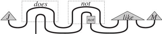
Figure 3: Diagram of Information Flow in the Negative Transitive Sentence

The ability to compute with diagrams is not lost in the move from compact to monoidal bi-closed categories. A diagrammatic calculus for these categories has been developed by Baez and Stay [6]. Similar to the graphical calculus of compact closed categories, the graphical calculus of monoidal bi-closed categories can be applied to both depict the grammatical reduction of Lambek monoids and the flow of information between meanings of the words in a sentence.

The basic constructs of the diagrammatic language of a monoidal bi-closed category are shown in Figures 4 and 5. We read these diagrams from top to bottom. Objects of the category are depicted by arrows. For instance the left hand side arrow of Figure 4 depicts object $A$. Morphisms of the category are depicted by ‘blobs’ with ‘input’ and ‘output’ arrows standing for their domain and codomain objects. The right hand side blob of Figure 4 depicts morphism $f$ which has domain $A$ and codomain $B$. Since an identity morphism has the same domain and codomain, it is depicted in the same way as the object corresponding to it. The identity morphism $id_{A}$ is denoted by the same diagram as that of object $A$, e.g in the left hand side diagram of Figure 4.

Figure 4: Basic Diagrammatic Language Constructs (1)

The tensor product of two objects corresponds to the side by side placement of their arrows, for instance the tensor product $A\otimes B$ of two objects $A$ and $B$ is depicted by putting the arrow depicting object $A$ beside the arrow depicting object $B$, as shown in the left hand side diagram of Figure 5. Right and left implications $A\multimap B$ and $A\multimapinv B$ are depicted by side by side placement and clasping of their arrows, pointing in opposite directions. For instance, the right implication $A\multimap B$ is depicted by putting the arrow corresponding to $A$ pointing upwards with the arrow corresponding to $B$ pointing downwards; with the arrow of $B$ being clasped to the arrow of $A$. The intuition behind the directions of the arrows is that in a right implication, the antecedent has a negative role and the consequence has a positive role; this reversal of roles is the reason behind the classical logical equivalence $A\to B\cong\neg A\vee B$. The clasp is a restriction: it is there to make us treat the implication as one entity and to prevent us from treating each of the arrows separately. As a result, for example, we cannot apply a function to one arrow, e.g. $A$ and not the other, e.g. $B$. The diagram corresponding to the left implication $A\multimapinv B$ is the opposite of that of the right implication. These two implications are depicted in the last two diagrams of Figure 5.

Figure 5: Basic Diagrammatic Language Constructs (2)

There might be more than one way of representing an object or morphism in this diagrammatic calculus. If so, these different ways are considered to be ‘equal’ and their resulting representations are considered to be ‘equivalent’. Figure 6 shows three of the main Baez-Stay diagrammatic equivalences. They express the fact that one can either draw the left hand side or equivalently the right hand side diagram to represent their corresponding morphism. For instance, one can either draw an arrow labeled with $A\otimes B$ for the tensor object $A\otimes B$ (or the identity arrow on it, i.e. $id_{A\otimes B}$) or two side-by-side arrows, one labeled with $A$ and the other with $B$. These equivalences are not the same as the equivalences of other diagrammatic calculi [55]. For instance, there is no connection between these and the coherence conditions of the category.

Figure 6: Equivalent Diagrammatic Representations

The equivalences for the left and right evaluations $ev^{l}$ and $ev^{r}$ are shown in Figure 7. Each of the diagrams of each equivalence input two arrows and output one arrow. The left hand side diagrams do not depict any information flow: they just show which objects the evaluation morphism is being applied to. The internal structure of the evaluation morphism is being depicted inside the blob of the right hand side diagrams. These diagrams depict how the information flows between an object and the implication, leading to an output. The flow represents the fact that, for instance, for the tensor product $A\otimes(A\multimap B)$ to be evaluated and to produce the output $B$, information has to flow from object $A$ to the antecedent of $A\multimap B$, and similarly for the left implication.

Figure 7: Diagrams for Left and Right Evaluation

The diagrams for left and right currying are shown in Figure 8. Here, the left hand side diagrams are the morphisms that are being curried and the right hand side diagrams depict the flow of information that happens in the process of currying. What happens outside the blob of the right hand side diagram has no flow and just lists the objects to which the currying morphism is being applied. The internal structure of the blobs depict the corresponding information flows. For instance, the diagram of $\Lambda^{l}(f)$ shows that in order to produce the morphism $C\to A\multimap B$, the information encoded in $A$ and $C$ have to flow to $f\colon(A\otimes C)\to B$. For this to happen, first $A$ has to detach itself from the clasp $A\multimap B$, a process that can only happen inside a blob.

Figure 8: Diagrams for Left and Right Currying

The diagrams for the equivalences corresponding to the evaluation of the names of morphisms, which lead to yanking, are shown in Figure 9 (note that in these diagrams we have stretched the caps inside the outer blobs for reasons of space). They show how, if we first curry $f$ to produce $A\multimap B$, then evaluate the result with $A$, the output will be the same as the output of applying $f$ to $A$, that is $B$.

Figure 9: Diagrams for Left and Right Yanking

8 Monoidal Bi-Closed Diagrams and Flow of Meaning in Language

The diagram of the intransitive sentence ‘men kill’ consists of just one evaluation: $ev^{l}_{n,s}$. It shows how information has to flow from the subject ‘men’ to the verb ‘kill’ to form the intransitive sentence ‘men kill’. In other words, the meaning of an intransitive sentence is obtained by applying its verb to its subject. The diagram for this application is depicted in Figure 10. For reasons of space, we use lowercase letters for both the grammatical types and their interpretation.

Figure 10: Diagram for ‘men kill’ and ‘men kill dogs’

For the transitive sentence ‘men kill dogs’, we first depict the subtype $n\multimap s$ of the verb with a single arrow and do an $ev^{r}_{n\multimap s,n}$ with the object. Then we use the equivalence for the right implication and replace the resulting object $n\multimap s$ with its equivalent clasped diagram which has two arrows of types $n$ and $s$ respectively. The replacement procedure is marked with a dotted line. At this point, we do an $ev^{l}_{n,s}$ on the implication diagram $n\multimap s$ and the subject $n$. The full diagram in Figure 10, shows that to obtain a meaning for a transitive sentence, information has to flow in two steps: first from the object ‘dogs’ to the verb ‘kill’ and then from the subject ‘men’ to the resulting verb phrase ‘kill dogs’. Note that this information flow was done in one step in the compact closed setting, where the subject and object interacted with the verb simultaneously and in one step. Whereas in the monoidal case, we have to wait for the verb to interact with the object before it can interact with the subject.

Figure 11: Diagram for ‘men kill cute dogs’

The diagram for the meaning of ‘men kill cute dogs’ is obtained by three evaluations, as depicted in Figure 11. Here, first the adjective acts on the object, then the verb acts on the resulting adjective-noun object to produce a verb phrase, which is then applied to the subject to produce a sentence. The corresponding diagrammatic computations are depicted in Figure 12. The left hand side diagram shows the verb phrase part of this interaction, whereby, ‘cute’ is applied to ‘dogs’ and then input to ‘kill’ as its object. The result is then applied to the meaning of ‘men’, this third application is depicted in the right hand side diagram, where the dotted area stands for the general structure of the first and second applications and serves as a shorthand for the left hand side diagram. The arrow between the two diagrams shows that the bottom left side of the first diagram is being inserted into the right hand side and acted upon.

Figure 12: Diagram for the Meaning of ‘men kill cute dogs’

The words whose meaning vectors are names of linear maps are obtained by currying the corresponding linear map. For instance, the meaning vector of the auxiliary ‘do’ is the name of the identity and the meaning vector of the negation word ‘not’ is the name of a negation operator, as specified in Section 6.2. The diagrams corresponding to the meaning vector of words that are names of certain morphisms are obtained by currying those morphisms. The diagrams of ‘does’ and ‘not’ are depicted in Figure 13.

Figure 13: Diagrams for ‘does’ and ‘not’

The meaning vector for ‘men do not kill dogs’ is obtained by substituting the diagrams of meanings of ‘does’ and ‘not’ into the diagram corresponding to the monoidal grammatical reduction of the sentence. The result is depicted in Figure 14. Here, the diagram on the right is the simplified version of the diagram on the left, where ‘kill’ has been applied to ‘dogs’ and the result has been inputted to ‘not’. This means that the result is being negated and the negation is then being applied to the meaning of ‘men’. As mentioned in Section 6.2, this procedure is different from the compact closed case and this difference, which basically lies in the order of applications, is manifested in the corresponding diagram of each case.

$\implies$      

Figure 14: Diagram for Meaning of ‘men do not kill dogs’

If Lambek monoids are interpreted in vector spaces, as demonstrated in the Section 6.2, they benefit from their extra compact structure, for instance symmetry of the tensor. Baez-Stay diagrams can easily be turned into compact string diagrams: by removing the clasp restrictions and popping the bubbles. There is, however, a problem: the resulting diagrams are not always the same as the compact diagrams that were originally drawn for sentences, as demonstrated in the above example. The problem stems from the restricted form of yanking in the monoidal case.

9 Concluding Remarks and Future Work

We have shown that the DisCoCat framework [13, 14] need not be committed to the grammatical formalism of Lambek pregroups [33], which are compact closed. Lambek monoids [31], which are monoidal closed, also allow a functorial passage to the category of finite dimensional vector spaces and the diagrammatic calculus of Baez and Stay [6] can be used to depict the information flow that happens within the sentences. This functorial passage is used in and referred to as quantisation in the context of Topological Quantum Field Theory (TQFT) [4, 5, 29]. As future work, we would like to (1) extend the results of this paper to richer type-logics, and (2) relate their diagrammatic calculi to Baez-Stay diagrams.

With regard to (1), we would like to develop distributional compositional models of meaning for richer grammars such as the Combinatorial Categorial Grammar [57] and Lambek-Grishin algebras [44, 8]. These grammars have more expressive power and can formalise larger fragments of natural language, and in particular English; CCG has been applied to parse large corpora of real data. To extend our quantisation functor from Lambek monoids to CCG, the cross composition rules need to be given a categorical semantics. This would perhaps require restricting the application of these rules to subcategories of the full type-category, as in their general forms, they do not hold either in a compact or a monoidal closed category. To extend the quantisation functor to Lambek-Grishin algebras, we need to ask the functor to preserve the operations of the Grishin part of the algebra, as well as their interactions with the Lambek part, hence defining functors that have to satisfy more than the monoidal conditions; the categorical properties of these functors should be studied. Whether or not such extensions prove to be trivial remains to be seen, but it is certain that augmenting the applicability of this general compositional categorical formalism will greatly assist its acceptance by the linguistic community as a practical theoretical toolkit.

As for (2), note that the general structure of Baez-Stay diagrams are the same as parse trees. This is not surprising given the Curry-Howard isomorphism between monoidal categories and lambda calculus [58]. Whereas parse trees are purely syntactical and only depict the grammatical structure of sentences, Baez-Stay diagrams have extra information in their nodes (blobs) about the flow of meaning and the semantic structure of phrases. The straight lines and the cups allow for a flow between the nodes they are connecting; this encodes the order and details of function applications. The clasps, however, stop this flow from happening, hence making it explicit which applications cannot happen. One can identify the clasps with lines and remove the cups to obtain a parse tree without this information. We have demonstrated this procedure for an example sentence in Figure 15; here, VP stands for an intransitive, transitive, or ditransitive verb phrases, and NP stands for a noun phrase.

Figure 15: Baez-Stay Diagrams and Parse Trees

The extra information in the blobs of Baez-Stay diagrams makes them more like proof nets. A proof net is a diagrammatic notation used to depict the grammatical structures of sentences and their lambda calculus meanings. Proof nets unify proofs, hence solve the spurious ambiguity problem and have been extensively studied by the linear logic [17] and linguistics communities [54, 46, 42]. They contain semantic information about sentences, represented by traverse instructions that describe how to form the lambda term corresponding to a grammatical reduction. These lambda terms can also be directly read from the sequent calculus proofs corresponding to the proof nets. An abstract form of proof nets, referred to as proof structures, encode semantic information about sentences to start with. These come equipped with certain contraction rules and can be rewritten to parse trees using these rules. The rewrites model the computations that provide us with the final meaning of the sentence. A formal connection between Baez-Stay diagrams and proof nets or structures constitutes future work. As one of the referees suggested, one possibility would be to develop a lambda calculus for Baez-Stay diagrams in the style of glue semantics [16].

10 Acknowledgement

We would like to thank Michael Moortgat, Glyn Morrill, Samson Abramsky, and Mike Stay for fruitful and clarifying discussions.

References

- [1] S. Abramsky. Temperley-lieb algebra: from knot theory to logic and computation via quantum mechanics. In Mathematics of quantum computation and quantum technology, Chapman and Hall/CRC Appl. Math. Nonlinear Sci. Ser., pages 515–558. Chapman and Hall/CRC, Boca Raton, FL, 2008.
- [2] S. Abramsky and B. Coecke. A categorical semantics of quantum protocols. In Proceedings of the 19th Annual IEEE Symposium on Logic in Computer Science, pages 415–425. IEEE Computer Science Press, 2004. arXiv:quant-ph/0402130.
- [3] S. Abramsky and R. Duncan. A categorical quantum logic. Mathematical Structures in Computer Science, 16(3):469–489, 2006.
- [4] M. Atiyah. Topological quantum field theories. Publications Mathématique de l’Institut des Hautes Études Scientifiques, 68:175–186, 1989.
- [5] J. Baez and J. Dolan. Higher-dimensional algebra and topological quantum field theory. Journal of Mathematical Physics, 36:6073 6105, 1995.
- [6] J. Baez and M. Stay. Physics, topology, logic, and computation: A rosetta stone. In B. Coecke, editor, New Structures in Physics, volume 813 of Lecture Notes in Physics. Springer, 2011.
- [7] Y. Bar-Hillel. A quasiarithmetical notation for syntactic description. Language, 29:47–58, 1953.
- [8] R. Bernardi and M. Moortgat. Continuation semantics for the lambek-grishin calculus. Information and Computation, 208:397–416, 2010.
- [9] W. Buszkowski. Lambek grammars based on pregroups. Logical Aspects of Computational Linguistics, 2001.
- [10] N. Chomsky. Aspects of the Theory of Syntax, volume 119. The MIT press, 1965.
- [11] S. Clark and S. Pulman. Combining symbolic and distributional models of meaning. In Proceedings of AAAI Spring Symposium on Quantum Interaction. AAAI Press, 2007.
- [12] B. Coecke. Kindergarten quantum mechanics — lecture notes. In A. Khrennikov, editor, Quantum Theory: Reconsiderations of the Foundations III, pages 81–98. AIP Press, 2005. arXiv:quant-ph/0510032.
- [13] B. Coecke, M. Sadrzadeh, and S. Clark. A compositional distributional model of meaning. In Proceedings of the Second Quantum Interaction Symposium, pages 133–140. College Press, 2008.
- [14] B. Coecke, M. Sadrzadeh, and S. Clark. Mathematical foundations for a compositional distributional model of meaning. Linguistic Analysis, 36(1–4):345–384, 2010.
- [15] J.R. Curran. From Distributional to Semantic Similarity. PhD thesis, University of Edinburgh, 2004.
- [16] M. Dalrymple. Semantics and syntax in Lexical Functional Grammar: The resource logic approach. MIT Press, 1999.
- [17] P. de Groote and C. Reotrè. On the semantic readings of proof nets. In D. Oehrle G.J. Kruijff, G. Morrill, editor, Proceedings of 2nd Formal Grammar Conference, 1996.
- [18] J.R. Firth. A synopsis of linguistic theory 1930-1955, volume 1952-59. The Philological Society, 1957.
- [19] G. Frege. Uber sinn und bedeutung. Zeitschrift für Philosophie und philosophische Kritik, 100(1):25–50, 1892.
- [20] O. Valentin G. Morrill and M. Fadda. The displacement calculus. Journal of Logic, Language and Information, 20:1–48, 2011.
- [21] E. Grefenstette and M. Sadrzadeh. Experimental support for a categorical compositional distributional model of meaning. In Proceedings of the Conference on Empirical Methods in Natural Language Processing, 2011.
- [22] E. Grefenstette and M. Sadrzadeh. Experimenting with transitive verbs in a discocat. In Proceedings of the EMNLP Workshop on Geometric Models of Natural Language Semantics, 2011.
- [23] G. Grefenstette. Explorations in Automatic Thesaurus Discovery. Kluwer, 1994.
- [24] J. Hintikka and G. Sandu. Game-theoretical semantics. In Handbook of Logic and Language, pages 361–410. MIT Press, 1997.
- [25] J.J. Jiang and D.W. Conrath. Semantic similarity based on corpus statistics and lexical taxonomy. arXiv preprint cmp-lg/9709008, 1997.
- [26] A. Joyal and R. Street. The geometry of tensor calculus I. Advances in Mathematics, 88:55–112, 1991.
- [27] M. Kelly and M. L. Laplaza. Coherence for compact closed categories. Journal of Pure and Applied Algebra, 19:193–213, 1980.
- [28] A. Kislak-Malinowska. Pregroups with modalities. In Shuly Wintner, editor, Proceedings of Formal Grammar Conference, 2006.
- [29] J. Kock. Frobenius Algebras and 2D Topological Quantum Field Theories. Cambridge University Press, 2003.
- [30] F. Lamarche and C. Retoré. Proof nets for the lambek calculus—an overview. In Proceedings of the Third Roma Workshop. Proofs and Linguistic Categories, pages 241–262, 1996.
- [31] J. Lambek. The mathematics of sentence structure. American Mathematics Monthly, 65, 1958.
- [32] J. Lambek. On some connections between logic and category theory. Studia Logica, 48:269–278, 1989.
- [33] J. Lambek. Type grammar revisited. Logical Aspects of Computational Linguistics, 1582, 1999.
- [34] J. Lambek. Iterated galois connections in arithmetics and linguistics. Galois Connections and Applications, Mathematics and its Applications, 565, 2004.
- [35] J. Lambek. From Word to Sentence. Polimetrica, 2008.
- [36] J. Lambek and C. Casadio, editors. Computational algebraic approaches to natural language. Polimetrica, Milan, 2006.
- [37] T. K. Landauer and S. T. Dumais. A solution to Plato’s problem: the latent semantic analysis theory of acquisition, induction and representation of knowledge. Psychological Review, 104(2):211–240, 1997.
- [38] J. A. Levin and J. A. Moore. Dialogue-games: metacommunication structures for natural language interaction. Cognitive Science, 1(4):395–420, 1977.
- [39] P. Lorenzen and K. Lorenz. Dialogische Logik. Wissenschaftliche Buchgesellschaft, 1978.
- [40] J. Mitchell and M. Lapata. Vector-based models of semantic composition. In Proceedings of the 46th Annual Meeting of the Association for Computational Linguistics, pages 236–244, 2008.
- [41] R. Montague. English as a formal language. Formal philosophy, pages 188–221, 1974.
- [42] M. Moortgat. Categorial investigations: Logical and Linguistic Aspects of the Lambek Calculus. Foris Publications, 1988.
- [43] M. Moortgat. Multimodal linguistic inference. Journal of Logic, Language and Information, 5(3/4):349–385, 1996.
- [44] M. Moortgat. Symmetric categorial grammar. Journal of Philosophical Logic, pages 681–710, 2009.
- [45] R. Moot. Proof Nets for Linguistic Analysis. PhD thesis, Utrecht Institute of Linguistics, 2002.
- [46] R. Moot and Q. Puite. Proof nets for the multimodal lambek calculus. Studia Logica, 71, 2002.
- [47] H. Ono, M. Kanazawa, and R. de Queiroz, editors. Logic, Language, Information and Computation, 16th International Workshop, WoLLIC 2009, Tokyo, Japan, June 21-24, 2009. Proceedings, volume 5514 of Lecture Notes in Computer Science. Springer, 2009.
- [48] R. Penrose. Applications of negative dimensional tensors. In Combinatorial Mathematics and its Applications, pages 221–244. Academic Press, 1971.
- [49] M. Pentus. Lambek grammars are context free. In Proceedings of the 8th Annual IEEE Symposium on Logic in Computer Science, pages 429–433, Los Alamitos, California, 1993. IEEE Computer Society Press.
- [50] A. Preller. Towards discourse representation via pregroup grammars. JoLLI, 2007.
- [51] A. Preller and J. Lambek. Free compact 2-categories. Mathematical Structures in Computer Science, 17(2):309–340, 2007.
- [52] A. Preller and M. Sadrzadeh. Bell states and negative sentences in the distributed model of meaning. In P. Selinger B. Coecke, P. Panangaden, editor, Electronic Notes in Theoretical Computer Science, Proceedings of the 6th QPL Workshop on Quantum Physics and Logic. University of Oxford, 2010.
- [53] S. G. Pulman. Conversational games, belief revision and bayesian networks. In J. Landsbergen et al., editor, CLIN VII: Proceedings of 7th Computational Linguistics in the Netherlands meeting, Nov 1996, pages 1–25, 1997.
- [54] D. Roorda. Proof nets for lambek calculus. Journal of Logic and Computation, 2, 1992.
- [55] P. Selinger. A survey of graphical languages for monoidal categories. In B. Coecke, editor, New structures for physics, Lecture Notes in Physics, pages 275–337. Springer, 2010.
- [56] P. Smolensky and G. Legendre. The Harmonic Mind: From Neural Computation to Optimality-Theoretic Grammar Vol. I: Cognitive Architecture Vol. II: Linguistic and Philosophical Implications. MIT Press, 2005.
- [57] M. Steedman. The syntactic process. The MIT press, 2001.
- [58] M. E. Szabo. Algebra of Proofs, volume 88 of Studies in Logic and the Foundations of Mathematics. North-Holland, 1978.
- [59] L. Wittgenstein. Philosophical investigations. Blackwell, 1953.