Bayesian Entropy Estimation for Countable Discrete Distributions

Abstract

We consider the problem of estimating Shannon’s entropy $H$ from discrete data, in cases where the number of possible symbols is unknown or even countably infinite. The Pitman-Yor process, a generalization of Dirichlet process, provides a tractable prior distribution over the space of countably infinite discrete distributions, and has found major applications in Bayesian non-parametric statistics and machine learning. Here we show that it also provides a natural family of priors for Bayesian entropy estimation, due to the fact that moments of the induced posterior distribution over $H$ can be computed analytically. We derive formulas for the posterior mean (Bayes’ least squares estimate) and variance under Dirichlet and Pitman-Yor process priors. Moreover, we show that a fixed Dirichlet or Pitman-Yor process prior implies a narrow prior distribution over $H$, meaning the prior strongly determines the entropy estimate in the under-sampled regime. We derive a family of continuous mixing measures such that the resulting mixture of Pitman-Yor processes produces an approximately flat prior over $H$. We show that the resulting Pitman-Yor Mixture (PYM) entropy estimator is consistent for a large class of distributions. We explore the theoretical properties of the resulting estimator, and show that it performs well both in simulation and in application to real data.

Keywords: entropy, information theory, Bayesian estimation, Bayesian nonparametrics, Dirichlet process, Pitman–Yor process, neural coding

1 Introduction

Shannon’s discrete entropy appears as a basic statistic in many fields, from probability theory to engineering and even ecology and neuroscience. While entropy may best be known as a theoretical quantity, its accurate estimation from data is an important part of many applications. For example, entropy is employed in the study of information processing in neuroscience, where the coding of neurons is typically unknown Strong et al. (1998); Barbieri et al. (2004); Shlens et al. (2007); Rolls et al. (1999). Entropy estimates are used to quantify the coding properties of a neural systems, such as the channel capacity, or form a step in computing other information-theoretic quantities, such as the mutual information. Entropy is also used in statistics and machine learning for estimating dependency structure and inferring causal relations Chow and Liu (1968); Schindler et al. (2007), for example in molecular biology Hausser and Strimmer (2009); as a tool in the study of complexity and dynamics in physics Letellier (2006); and as a measure of diversity in ecology Chao and Shen (2003) and genetics Farach et al. (1995). Each of these studies, confronted with data arising from an unknown discrete distribution, seeks to estimate the entropy rather than the distribution itself. The reason for this, fundamentally, is the difficulty of density estimation: it may not be feasible to collect enough data to usefully estimate the full distribution. The problem is not just that we may not have enough data to estimate the frequency of an event accurately. In the so-called “undersampled regime”, we may not even observe all events that have non-zero frequency. In general, estimating a density in this setting is a hopeless endeavor.

Estimating the entropy is much easier than estimating the full distribution. In fact, in many cases, entropy can be accurately estimated with fewer samples than the number of distinct symbols. Nevertheless, entropy estimation remains a difficult problem: there is no unbiased estimator for entropy, and the maximum likelihood estimator is severely biased for small datasets Paninski (2003). Many previous studies have focused upon methods for computing and reducing this bias Miller (1955); Panzeri and Treves (1996); Strong et al. (1998); Paninski (2003); Grassberger (2008). In this paper we instead take a Bayesian approach, building upon the work of Nemenman et al. (2002). Our basic strategy is to place a prior over the space of discrete probability distributions, and then perform inference using the induced posterior distribution over entropy. (See Fig. 1).

We focus on the under-sampled regime, where the number of unique symbols observed in the data is small in comparison with an unknown (perhaps infinite) number of possible symbols. While the true distribution underlying any real dataset is undoubtedly finite, formulating a model on the space of infinite-dimensional distributions allows us to be agnostic about the true cardinality. This assumption leads to a convenient and tractable estimator that converges to the true entropy even when the maximal support of the distribution is known to be finite. As an example, consider an arbitrary distribution over $N$-grams on a binary alphabet. While there are at most $2^{N}$ symbols, the true cardinality of the response distribution is generally unknown to the experimenter. A given distribution may be supported on any number of symbols less than $2^{N}$. In some applications, there may not even be a known upper bound on the number of symbols (e.g., the problem of estimating the number of undiscovered species in a given region). By using a prior with support for countably infinite distributions, our model does not require a priori specification of the alphabet size.

The Pitman-Yor process (PYP), a two-parameter generalization of the Dirichlet process (DP) Pitman and Yor (1997); Ishwaran and James (2003); Goldwater et al. (2006), provides an attractive family of priors in this setting, since: (1) the posterior distribution over entropy has analytically tractable moments; and (2) distributions drawn from a PYP can exhibit power-law tails, a feature commonly observed in data from social, biological, and physical systems Zipf (1949); Dudok de Wit (1999); Newman (2005).

We show that a PYP prior with fixed hyperparameters imposes a narrow prior distribution over entropy, leading to severe bias and overly narrow posterior credible intervals given a small dataset. Our approach, inspired by Nemenman et al. (2002), is to introduce a family of mixing measures over Pitman-Yor processes such that the resulting Pitman-Yor Mixture (PYM) prior provides an approximately non-informative (i.e., flat) prior over entropy.

The remainder of the paper is organized as follows. In Section 2, we introduce the entropy estimation problem and review prior work. In Section 3, we introduce the Dirichlet and Pitman-Yor processes and discuss key mathematical properties relating to entropy. In Section 4, we introduce a novel entropy estimator based on PYM priors and derive several of its theoretical properties. In Section 5, we show compare various estimators with applications to data.

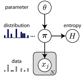
Figure 1: Graphical model illustrating the ingredients for Bayesian entropy estimation. Arrows indicate conditional dependencies between variables, and the gray “plate” denotes multiple copies of a random variable (with the number of copies $N$ indicated at bottom). For entropy estimation, the joint probability distribution over entropy $H$, data ${\mathbf{x}}=\{x_{j}\}$, discrete distribution ${\bm{\pi}}=\{\pi_{i}\}$, and parameter $\theta$ factorizes as: $p(H,{\mathbf{x}},{\bm{\pi}},\theta)=p(H|{\bm{\pi}})p({\mathbf{x}}|{\bm{\pi}})p({\bm{\pi}}|\theta)p(\theta)$. Entropy is a deterministic function of ${\bm{\pi}}$, so $p(H|{\bm{\pi}})=\delta(H-\sum_{i}\pi_{i}\log\pi_{i}).$ The Bayes least squares estimator corresponds to the posterior mean: $\mathbb{E}[H|{\mathbf{x}}]=\iint p(H|{\bm{\pi}})p({\bm{\pi}},\theta|{\mathbf{x}})d{\bm{\pi}}\,d\theta$.

2 Entropy Estimation

Consider samples ${\mathbf{x}}:=\left\{x_{j}\right\}_{j=1}^{N}$ drawn iid from an unknown discrete distribution ${\bm{\pi}}:=\left\{\pi_{i}\right\}_{i=1}^{\mathcal{A}}$, $p(x_{j}=i)=\pi_{i}$, on a finite or (countably) infinite alphabet $\mathcal{X}$ with cardinality $\mathcal{A}$. We wish to estimate the entropy of ${\bm{\pi}}$,

$$H({\bm{\pi}})=-\sum_{i=1}^{\mathcal{A}}\pi_{i}\log\pi_{i}.$$ (1)

We are interested in the “undersampled regime”, $N\ll\mathcal{A}$, where many of the symbols remain unobserved. We will see that a naive approach to entropy estimation in this regime results in severely biased estimators, and briefly review approaches for correcting this bias. We then consider Bayesian techniques for entropy estimation in general before introducing the Nemenman–Shafee–Bialek (NSB) method upon which the remainder of the article will build.

2.1 Plugin estimator and bias-correction methods

Perhaps the most straightforward entropy estimation technique is to estimate the distribution ${\bm{\pi}}$ and then use the plugin formula (1) to evaluate its entropy. The empirical distribution $\hat{\bm{\pi}}=(\hat{\pi}_{1},\ldots,\hat{\pi}_{\mathcal{A}})$ is computed by normalizing the observed counts ${\mathbf{n}}:=(n_{1},\ldots,n_{\mathcal{A}})$ of each symbol,

$$\hat{\pi}_{k}=n_{k}/N,\qquad n_{k}=\sum_{i=1}^{N}\mathbf{1}_{\left\{x_{i}=k\right\}},$$ (2)

for each $k\in\mathcal{X}$. Plugging this estimate for ${\bm{\pi}}$ into (1), we obtain the so-called “plugin” estimator:

$$\hat{H}_{\text{plugin}}=-\sum\hat{\pi}_{i}\log\hat{\pi}_{i},$$ (3)

which is also the maximum-likelihood estimator under categorical (or multinomial) likelihood.

Despite its simplicity and desirable asymptotic properties, $\hat{H}_{\text{plugin}}$ exhibits substantial negative bias in the undersampled regime. There exists a large literature on methods for removing this bias, much of which considers the setting in which $\mathcal{A}$ is known and finite. One popular and well-studied method involves taking a series expansion of the bias Miller (1955); Treves and Panzeri (1995); Panzeri and Treves (1996); Grassberger (2008) and then subtracting it from the plugin estimate. Other recent proposals include minimizing an upper bound over a class of linear estimators Paninski (2003), and a James-Stein estimator Hausser and Strimmer (2009). Recent work has also considered countably infinite alphabets. The coverage-adjusted estimator (CAE) Chao and Shen (2003); Vu et al. (2007) addresses bias by combining the Horvitz-Thompson estimator with a nonparametric estimate of the proportion of total probability mass (the “coverage”) accounted for by the observed data ${\mathbf{x}}$. In a similar spirit, Zhang (2012) proposed an estimator based on the Good-Turing estimate of population size.

2.2 Bayesian entropy estimation

The Bayesian approach to entropy estimation involves formulating a prior over distributions ${\bm{\pi}}$, and then turning the crank of Bayesian inference to infer $H$ using the posterior distribution. Bayes’ least squares (BLS) estimators take the form:

$$\hat{H}({\mathbf{x}})=\mathbb{E}[H|{\mathbf{x}}]=\int H({\bm{\pi}})p(H|{\bm{\pi}})p({\bm{\pi}}|{\mathbf{x}})\,\mathrm{d}{\bm{\pi}},$$ (4)

where $p({\bm{\pi}}|{\mathbf{x}})$ is the posterior over ${\bm{\pi}}$ under some prior $p({\bm{\pi}})$ and discrete likelihood $p({\mathbf{x}}|{\bm{\pi}})$, and

$$p(H|{\bm{\pi}})=\delta(H+\sum_{i}\pi_{i}\log\pi_{i}),$$ (5)

since $H$ is deterministically related to ${\bm{\pi}}$. To the extent that $p({\bm{\pi}})$ expresses our true prior uncertainty over the unknown distribution that generated the data, this estimate is optimal (in a least-squares sense), and the corresponding credible intervals capture our uncertainty about $H$ given the data.

For distributions with known finite alphabet size $\mathcal{A}$, the Dirichlet distribution provides an obvious choice of prior due to its conjugacy with the categorical distribution. It takes the form

$$p_{Dir}({\bm{\pi}})\propto\prod_{i=1}^{\mathcal{A}}\pi_{i}^{{a}-1},$$ (6)

for ${\bm{\pi}}$ on the ${\mathcal{A}}$-dimensional simplex ($\pi_{i}\geq 1$, $\sum\pi_{i}=1$), where ${a}>0$ is a “concentration” parameter Hutter (2002). Many previously proposed estimators can be viewed as Bayesian under a Dirichlet prior with particular fixed choice of ${a}$. See Hausser and Strimmer (2009) for a historical overview of entropy estimators arising from specific choices of ${a}$.

2.3 Nemenman-Shafee-Bialek (NSB) estimator

In a seminal paper, Nemenman et al. (2002) showed that for finite distributions with known $\mathcal{A}$, Dirichlet priors with fixed ${a}$ impose a narrow prior distribution over entropy. In the undersampled regime, Bayesian estimates based on such highly informative priors are essentially determined by the value of ${a}$. Moreover, they have undesirably narrow posterior credible intervals, reflecting narrow prior uncertainty rather than strong evidence from the data. (These estimators generally give incorrect answers with high confidence!). To address this problem, Nemenman et al. (2002) suggested a mixture-of-Dirichlets prior:

$$p({\bm{\pi}})=\int p_{\mathrm{Dir}}({\bm{\pi}}|{a})p({a})\,\mathrm{d}{{a}},$$ (7)

where $p_{\mathrm{Dir}}({\bm{\pi}}|{a})$ denotes a $\mathrm{Dir}({a})$ prior on ${\bm{\pi}}$, and $p({a})$ denotes a set of mixing weights, given by

$$p({a})\propto\frac{d}{d{a}}\mathbb{E}[H|{a}]=\mathcal{A}\psi_{1}(\mathcal{A}{a}+1)-\psi_{1}({a}+1),$$ (8)

where $\mathbb{E}[H|{a}]$ denotes the expected value of $H$ under a $\mathrm{Dir}({a})$ prior, and $\psi_{1}(\cdot)$ denotes the tri-gamma function. To the extent that $p(H|{a})$ resembles a delta function, (7) and (8) imply a uniform prior for $H$ on $[0,\log\mathcal{A}]$. The BLS estimator under the NSB prior can be written:

$$\hat{H}_{nsb} =\mathbb{E}[H|{\mathbf{x}}]=\iint H({\bm{\pi}})p({\bm{\pi}}|{\mathbf{x}},{a})\,p({a}|{\mathbf{x}})\,\mathrm{d}{{\bm{\pi}}}\,\mathrm{d}{{a}}$$

$$=\int\mathbb{E}[H|{\mathbf{x}},{a}]\frac{p({\mathbf{x}}|{a})p({a})}{p({\mathbf{x}})}\,\,\mathrm{d}{{a}},$$ (9)

where $E[H|{\mathbf{x}},{a}]$ is the posterior mean under a $\mathrm{Dir}({a})$ prior, and $p({\mathbf{x}}|{a})$ denotes the evidence, which has a Pólya distribution Minka (2003):

$$p({\mathbf{x}}|{a}) =\int p({\mathbf{x}}|{\bm{\pi}})p({\bm{\pi}}|{a})\,\mathrm{d}{{\bm{\pi}}}$$

$$=\frac{(N!)\Gamma(\mathcal{A}{a})}{\Gamma({a})^{\mathcal{A}}\Gamma(N+\mathcal{A}{a})}\prod_{i=1}^{\mathcal{A}}\frac{\Gamma(n_{i}+{a})}{n_{i}!}.$$ (10)

The NSB estimate $\hat{H}_{nsb}$ and its posterior variance are fast to compute via 1D numerical integration in ${a}$ using closed-form expressions for the first two moments of the posterior distribution of $H$ given ${a}$. The forms for these moments are discussed in Wolpert and Wolf (1995); Nemenman et al. (2002), but the full formulae are not explicitly shown. Here we state the results:

$$\mathbb{E}[H|{\mathbf{x}},{a}] =\psi_{0}(\tilde{N}+1)-\sum_{i}\frac{\tilde{n}_{i}}{\tilde{N}}\psi_{0}(\tilde{n}_{i}+1)$$ (11)

$$\mathbb{E}[H^{2}|{\mathbf{x}},{a}] =\sum_{i\neq k}\frac{\tilde{n}_{i}\tilde{n}_{k}}{(\tilde{N}+1)\tilde{N}}I_{i,k}+\sum_{i}\frac{(\tilde{n}_{i}+1)\tilde{n}_{i}}{(\tilde{N}+1)\tilde{N}}J_{i}$$ (12)

$$I_{i,k} =\left(\psi_{0}(\tilde{n}_{k}+1)-\psi_{0}(\tilde{N}+2)\right)\left(\psi_{0}(\tilde{n}_{i}+1)-\psi_{0}(\tilde{N}+2)\right)-\psi_{1}(\tilde{N}+2)$$

$$J_{i} =(\psi_{0}(\tilde{n}_{i}+2)-\psi_{0}(\tilde{N}+2))^{2}+\psi_{1}(\tilde{n}_{i}+2)-\psi_{1}(\tilde{N}+2),$$

where $\tilde{n}_{i}=n_{i}+{a}$ are counts plus prior “pseudocount” ${a}$, $\tilde{N}=\sum\tilde{n}_{i}$ is the total of counts plus pseudocounts, and $\psi_{n}$ is the polygamma of $n$-th order (i.e., $\psi_{0}$ is the digamma function). Finally, $\operatorname*{var}[H|{\mathbf{n}},{a}]=\mathbb{E}[H^{2}|{\mathbf{n}},{a}]-\mathbb{E}[H|{\mathbf{n}},{a}]^{2}$. We derive these formulae in the Appendix, and in addition provide an alternative derivation using a size-biased sampling formulae discussed in Section 3.

2.4 Asymptotic NSB estimator

Nemenman et al. have proposed an extension of the NSB estimator to countably infinite distributions (or distributions with unknown cardinality), using a zeroth order approximation to $\hat{H}_{nsb}$ in the limit $\mathcal{A}\to\infty$ which we refer to as asymptotic-NSB (ANSB) Nemenman et al. (2004); Nemenman (2011),

$$\hat{H}_{ansb}=2\log(N)+\psi_{0}(N-K)-\psi_{0}(1)-\log(2),$$ (13)

where $K$ is the number of distinct symbols in the sample. Note that the ANSB estimator is designed specifically for an extremely undersampled regime ($K\sim N$), which we refer to as the “ANSB approximation regime”. The fact that ANSB diverges with $N$ in the well-sampled regime (as noted by [Vu07]) is therefore consistent with its design. In our experiments with ANSB in subsequent sections, we follow Nemenman (2011) and define the ANSB approximation regime to be that region such that $E[K_{N}]/N>0.9$, where $K_{N}$ is the number of unique symbols appearing in a sample of size $N$.

3 Dirichlet and Pitman-Yor Process Priors

To construct a prior over unknown or countably infinite discrete distributions, we borrow tools from nonparametric Bayesian statistics. The Dirichlet Process (DP) and Pitman-Yor process (PYP) define stochastic processes whose samples are countably infinite discrete distributions Ferguson (1973); Pitman and Yor (1997). A sample from a DP or PYP may be written as $\sum_{i=1}^{\infty}\pi_{i}\delta_{\phi_{i}}$, where now ${\bm{\pi}}=\{\pi_{i}\}$ denotes a countably infinite set of ‘weights’ on a set of atoms $\{\phi_{i}\}$ drawn from some base probability measure, where $\delta_{\phi_{i}}$ is a delta function on the atom $\phi_{i}$. We use DP and PYP to define a prior distribution on the infinite-dimensional simplex. The prior distribution over ${\bm{\pi}}$ under the DP or PYP is technically called the GEM distribution or the two-parameter Poisson-Dirichlet distribution, but we will abuse terminology by referring to both the process and its associated weight distribution by the same symbol, DP or PY Ishwaran and Zarepour (2002).

The DP distribution over ${\bm{\pi}}$ results from a limit of the (finite) Dirichlet distribution where alphabet size grows and concentration parameter shrinks: $\mathcal{A}\rightarrow\infty$ and ${a}\rightarrow 0$ s.t. ${a}\mathcal{A}\rightarrow{\alpha}$. The PYP distribution over ${\bm{\pi}}$ generalizes the DP to allow power-law tails, and includes DP as a special case Kingman (1975); Pitman and Yor (1997). For ${\mbox{PY}}(d,{\alpha})$ with $d\neq 0$, the tails approximately follow a power-law: $\pi_{i}\propto\left(i\right)^{-\frac{1}{d}}$ (pp. 867, Pitman and Yor (1997)). Many natural phenomena such as city size, language, spike responses, etc., also exhibit power-law tails Zipf (1949); Newman (2005). Fig. 2 shows two such examples, along with a sample drawn from the best-fitting DP and PYP distributions.

Let ${\mbox{PY}}(d,{\alpha})$ denote the PYP with discount parameter $d$ and concentration parameter ${\alpha}$ (also called the “Dirichlet parameter”), for $d\in[0,1),{\alpha}>-d$. When $d=0$, this reduces to the Dirichlet process, ${\mbox{DP}}({\alpha})$. To gain intuition for the DP and PYP, it is useful to consider typical samples ${\bm{\pi}}$ with weights $\{\pi_{i}\}$ sorted in decreasing order of probability, so that $\pi_{(1)}>\pi_{(2)}>\cdots$. The concentration parameter ${\alpha}$ controls how much of the probability mass is concentrated in the first few samples, that is, in the head instead of the tail of the sorted distribution. For small ${\alpha}$, the first few weights carry most of the probability mass, whereas for large ${\alpha}$, the probability mass is more spread out so that ${\bm{\pi}}$ is more uniform. As noted above, the discount parameter $d$ controls the shape of the tail, with larger $d$ giving heavier power-law tails, and $d=0$ giving exponential tails.

We can draw samples ${\bm{\pi}}\sim{\mbox{PY}}(d,{\alpha})$ using an infinite sequence of independent Beta random variables in a process known as “stick-breaking” Ishwaran and James (2001):

$$\beta_{i}\sim\mathrm{Beta}(1-d,{\alpha}+id),\qquad\tilde{\pi}_{i}=\prod_{j=1}^{i-1}(1-\beta_{j})\beta_{i},$$ (14)

where $\tilde{\pi}_{i}$ is known as the $i$’th size-biased permutation from ${\bm{\pi}}$ Pitman (1996). The $\tilde{\pi}_{i}$ sampled in this manner are not strictly decreasing, but decrease on average such that $\sum_{i=1}^{\infty}\tilde{\pi}_{i}=1$ with probability 1 Pitman and Yor (1997).

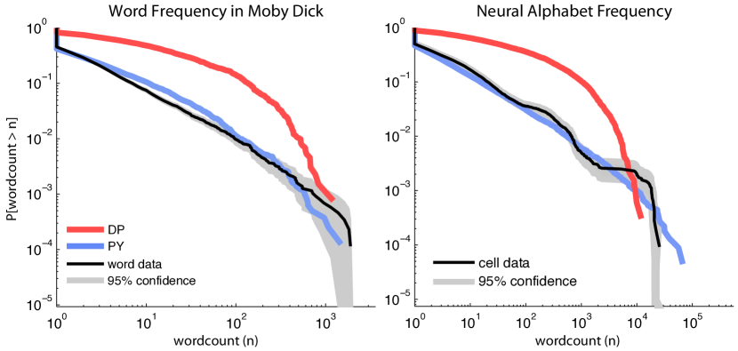
Figure 2: Empirical cumulative distribution functions of words in natural language (above) and neural spike patterns (below). We compare samples from the DP (red) and PYP (blue) priors for two datasets with heavy tails (black). In both cases, we compare the empirical CDF estimated from data to distributions drawn from DP and PYP using the ML values of ${\alpha}$ and $(d,{\alpha})$, respectively. For both datasets, PYP better captures the heavy-tailed behavior of the data. Left: Frequency of $N=217826$ words in the novel Moby Dick by Herman Melville. Right: Frequencies among $N=1.2\times 10^{6}$ neural spike words from $27$ simultaneously-recorded retinal ganglion cells, binarized and binned at 10ms.

3.1 Expectations over DP and PYP priors

A key virtue of PYP priors for our purposes is a mathematical property called invariance under size-biased sampling, which allows us to convert expectations over ${\bm{\pi}}$ on the infinite-dimensional simplex (which are required for computing the mean and variance of $H$ given data) into one- or two-dimensional integrals with respect to the distribution of the first two size-biased samples Perman et al. (1992); Pitman (1996).

Proposition 1 (Expectations with first two size-biased samples)

For ${\bm{\pi}}\sim{\mbox{PY}}(d,{\alpha})$,

$$\mathbb{E}_{({\bm{\pi}}|d,{\alpha})}\left[\sum_{i=1}^{\infty}f(\pi_{i})\right] =\mathbb{E}_{(\tilde{\pi}_{1}|d,{\alpha})}\left[\frac{f(\tilde{\pi}_{1})}{\tilde{\pi}_{1}}\right],$$ (15)

$$\mathbb{E}_{({\bm{\pi}}|d,{\alpha})}\left[\sum_{i,j\neq i}g(\pi_{i},\pi_{j})\right] =\mathbb{E}_{(\tilde{\pi}_{1},\tilde{\pi}_{2}|d,{\alpha})}\left[\frac{g(\tilde{\pi}_{1},\tilde{\pi}_{2})}{\tilde{\pi}_{1}\tilde{\pi}_{2}}(1-\tilde{\pi}_{1})\right],$$ (16)

where $\tilde{\pi}_{1}$ and $\tilde{\pi}_{2}$ are the first two size-biased samples from ${\bm{\pi}}$.

The first result (15) appears in Pitman and Yor (1997), and an analogous proof can be constructed for (16) (see Appendix).

The direct consequence of this proposition is that the first two moments of $H({\bm{\pi}})$ under the PYP and DP priors have closed forms ,

$$\mathbb{E}[H|d,{\alpha}] ={\psi_{0}}({\alpha}+1)-{\psi_{0}}(1-d),$$ (17)

$$\operatorname*{var}[H|d,{\alpha}] =\frac{{\alpha}+d}{({\alpha}+1)^{2}(1-d)}+\frac{1-d}{{\alpha}+1}\psi_{1}(2-d)-\psi_{1}(2+{\alpha}).$$ (18)

The derivation can be found in the appendix.

3.2 Expectations over DP and PYP posteriors

A useful property of PYP priors (for multinomial observations) is that the posterior $p({\bm{\pi}}|{\mathbf{x}},d,{\alpha})$ takes the form of a mixture of a Dirichlet distribution (over the observed symbols) and a Pitman-Yor process (over the unobserved symbols) Ishwaran and James (2003). This makes the integrals over the infinite-dimensional simplex tractable, and as a result we obtain closed-form solutions for the posterior mean and variance of $H$. Let $K$ be the number of unique symbols observed in $N$ samples, i.e., $K=\sum_{i=1}^{\mathcal{A}}\mathbf{1}_{\left\{n_{i}>0\right\}}$. Further, let ${\alpha}_{i}=n_{i}-d$, $N=\sum n_{i}$, and $A=\sum{\alpha}_{i}=\sum_{i}n_{i}-Kd=N-Kd$. Now, following Ishwaran and Zarepour (2002) we write the posterior as an infinite random vector ${\bm{\pi}}|{\mathbf{x}},d,{\alpha}=(p_{1},p_{2},p_{3},\dots,p_{K},p_{\ast}{\bm{\pi}}^{\prime})$, where

$$(p_{1},p_{2},\dots,p_{K},p_{\ast}) \sim\mathrm{Dir}(n_{1}-d,\dots,n_{K}-d,{\alpha}+Kd)$$ (19)

$${\bm{\pi}}^{\prime}:=(\pi_{1},\pi_{2},\pi_{3},\dots) \sim{\mbox{PY}}(d,{\alpha}+Kd).$$

The posterior mean $E[H|{\mathbf{x}},d,{\alpha}]$ is given by,

$$\mathbb{E}[H|{\alpha},d,{\mathbf{x}}]=\psi_{0}({\alpha}+N+1)-\frac{{\alpha}+Kd}{{\alpha}+N}\psi_{0}(1-d)-\frac{1}{{\alpha}+N}\left[\sum_{i=1}^{K}(n_{i}-d)\psi_{0}(n_{i}-d+1)\right].$$ (20)

The variance, $\operatorname*{var}[H|{\mathbf{x}},d,{\alpha}]$, also has an analytic closed form which is fast to compute. As we discuss in detail in Appendix A.4, $\operatorname*{var}[H|{\mathbf{x}},d,{\alpha}]$ may be expressed in terms of the first two moments of $p_{\ast}$, ${\bm{\pi}}$, and $\mathbf{p}=(p_{1},\ldots,p_{K})$ appearing in the posterior (19). Applying the law of total variance and using the independence properties of the posterior, we find:

$$\operatorname*{var}[H|d,{\alpha}] =\mathbb{E}_{p_{\ast}}[(1-p_{\ast})^{2}]\operatorname*{var}_{\mathbf{p}}[H(\mathbf{p})]+\mathbb{E}_{p_{\ast}}[p_{\ast}^{2}]\operatorname*{var}_{{\bm{\pi}}}[H({\bm{\pi}})]$$

$$\quad+\mathbb{E}_{p_{\ast}}[\Omega^{2}(p_{\ast})]-\mathbb{E}_{p_{\ast}}[\Omega(p_{\ast})]^{2},$$ (21)

where $\Omega(p_{\ast})=(1-p_{\ast})\mathbb{E}_{\mathbf{p}}\left[H(\mathbf{p})\right]+p_{\ast}\mathbb{E}_{{\bm{\pi}}}\left[H({\bm{\pi}})\right]+H(p_{\ast})$, and $H(p_{\ast})=-p_{\ast}\log(p_{\ast})-(1-p_{\ast})\log(1-p_{\ast})$. To specify $\Omega(p_{\ast})$, we let $\mathbf{A}=\mathbb{E}_{\mathbf{p}}\left[H(\mathbf{p})\right]$, $\mathbf{B}=\mathbb{E}_{{\bm{\pi}}}\left[H({\bm{\pi}})\right]$ so that,

$$\mathbb{E}[\Omega] =\mathbb{E}_{p_{\ast}}[1-p_{\ast}]\mathbb{E}_{\mathbf{p}}\left[H(\mathbf{p})\right]+\mathbb{E}_{p_{\ast}}[p_{\ast}]\mathbb{E}_{{\bm{\pi}}}\left[H({\bm{\pi}})\right]+H(p_{\ast}),$$

$$\mathbb{E}[\Omega^{2}] =2\mathbb{E}_{p_{\ast}}[p_{\ast}H(p_{\ast})][\mathbf{B}-\mathbf{A}]+2\mathbf{A}\mathbb{E}_{p_{\ast}}[H(p_{\ast})]+\mathbb{E}_{p_{\ast}}[h^{2}(p_{\ast})]$$

$$+\mathbb{E}_{p_{\ast}}[p_{\ast}^{2}]\left[\mathbf{B}^{2}-2\mathbf{A}\mathbf{B}\right]+2\mathbb{E}_{p_{\ast}}[p_{\ast}]\mathbf{A}\mathbf{B}+\mathbb{E}_{p_{\ast}}[(1-p_{\ast})^{2}]\mathbf{A}^{2}.$$

4 Entropy inference under DP and PYP priors

The posterior expectations computed in Section 3.2 provide a class of entropy estimators for distributions with countably-infinite support. For each choice of $(d,{\alpha})$, $\mathbb{E}[H|{\alpha},d,{\mathbf{x}}]$ is the posterior mean under a $PY(d,{\alpha})$ prior, analogous to the fixed-${\alpha}$ Dirichlet priors discussed in Section 2.2. Unfortunately, fixed $PY(d,{\alpha})$ priors also carry the same difficulties as fixed Dirichlet priors. A fixed-parameter ${\mbox{PY}}(d,{\alpha})$ prior on ${\bm{\pi}}$ results in a highly concentrated prior distribution on entropy (Fig. 3).

We address this problem by introducing a mixture prior $p(d,{\alpha})$ on ${\mbox{PY}}(d,{\alpha})$ under which the implied prior on entropy is flat. We then define the BLS entropy estimator under this mixture prior, the Pitman-Yor Mixture (PYM) estimator, and discuss some of its theoretical properties. Finally, we turn to the computation of PYM, discussing methods for sampling, and numerical quadrature integration.

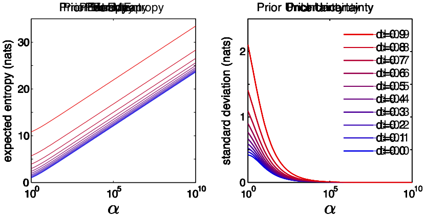
Figure 3: Prior entropy mean and variance (17) and 18 as a function of ${\alpha}$ and $d$. Note that entropy is approximately linear in $\log{\alpha}$. For large values of ${\alpha}$, $p(H({\bm{\pi}})|d,{\alpha})$ is highly concentrated around the mean.

4.1 Pitman-Yor process mixture (PYM) prior

One way of constructing a flat mixture prior is to follow the approach of Nemenman et al. (2002) by setting $p(d,{\alpha})$ proportional to the derivative of the expected entropy (17). Unlike NSB, we have two parameters through which to control the prior expected entropy. For instance, large prior (expected) entropies can arise either from large values of ${\alpha}$ (as in the DP) or from values of $d$ near 1 (see Fig. 3A). We can explicitly control this trade-off by reparameterizing PYP as follows,

$$h={\psi_{0}}({\alpha}+1)-{\psi_{0}}(1-d),\quad\gamma=\frac{{\psi_{0}}(1)-{\psi_{0}}(1-d)}{{\psi_{0}}({\alpha}+1)-{\psi_{0}}(1-d)},$$ (22)

where $h>0$ is equal to the expected prior entropy (17), and $\gamma\in[0,\infty)$ captures prior beliefs about tail behavior (Fig. 4A). For $\gamma=0$, we have the DP (i.e., $d=0$, giving ${\bm{\pi}}$ with exponential tails), while for $\gamma=1$ we have a ${\mbox{PY}}(d,0)$ process (i.e., ${\alpha}=0$, yielding ${\bm{\pi}}$ with power-law tails). In the limit where $\alpha\to-1$ and $d\to 1$, $\gamma\to\infty$. Where required, the inverse transformation to standard PY parameters is given by: ${\alpha}={\psi_{0}}^{-1}\left(h(1-\gamma)+{\psi_{0}}(1)\right)-1$, $d=1-{\psi_{0}}^{-1}\left({\psi_{0}}(1)-h\gamma\right),$ where ${\psi_{0}}^{-1}(\cdot)$ denotes the inverse digamma function.

We can construct an (approximately) flat improper distribution over $H$ on $[0,\infty]$ by setting $p(h,\gamma)=q(\gamma)$ for all $h$, where $q$ is any density on $[0,\infty)$. We call this the Pitman-Yor process mixture (PYM) prior. The induced prior on entropy is thus:

$$p(H)=\iint p(H|{\bm{\pi}})p({\bm{\pi}}|\gamma,h)p(\gamma,h)\,\mathrm{d}{\gamma}\,\mathrm{d}{h},$$ (23)

where $p({\bm{\pi}}|\gamma,h)$ denotes a PYP on ${\bm{\pi}}$ with parameters $\gamma,h$. We compare only three choices of $q(\gamma)$ here. However, the prior $q(\gamma)$ is not fixed, but may be adapted to reflect prior beliefs about the dataset at hand. A $q(\gamma)$ that places probability mass on larger $\gamma$ (near $1$) results in a prior that prefers heavy-tailed behavior and high entropy, whereas weight on small $\gamma$ prefers exponential-tailed distributions. As a result, priors with more mass on large $\gamma$ will also tend to yield wider credible intervals and higher estimates of entropy. PYM mixture priors resulting from different choices of $q(\gamma)$ are all approximately flat on $H$, but each favors distributions with different tail behavior; the ability to select $q(\gamma)$ greatly enhances the flexibility of PYM, allowing the practitioner to adapt it to her own data.

Fig. 4B shows samples from this prior under three different choices of $q(\gamma)$, for $h$ uniform on $[0,3]$. For the experiments, we use $q(\gamma)=\exp(-\frac{10}{1-\gamma})\mathbf{1}_{\{\gamma<1\}}$ which yields good results by weighting less on extremely heavy-tailed distributions. Combined with the likelihood, the posterior $p(d,{\alpha}|{\mathbf{x}})\propto p({\mathbf{x}}|d,{\alpha})p(d,{\alpha})$ quickly concentrates as more data are given, as demonstrated in Fig. 5.

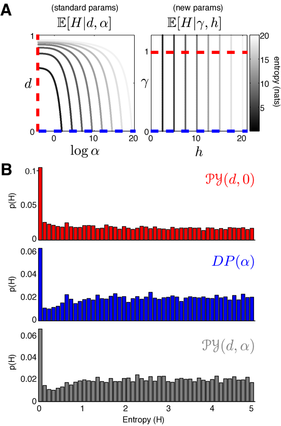
Figure 4: Prior over expected entropy under Pitman-Yor process prior. (A) Left: expected entropy as a function of the natural parameters $(d,{\alpha})$. Right: expected entropy as a function of transformed parameters $(h,\gamma)$. (B) Sampled prior distributions ($N=5e3$) over entropy implied by three different PYM priors over $\alpha$ and $d$. Each PYM prior is a mixture of a different PYP: ${\mbox{PY}}(d,0)$ (red), ${\mbox{PY}}(d,{\alpha})$ (grey), and ${\mbox{PY}}(0,{\alpha})={\mbox{DP}}({\alpha})$ (blue). Note that the “true” $p(H)$ is an improper prior supported on $[0,\infty)$. We visualize the sampled distributions only on the range from $0$ to $5$ nats, since sampling from PY becomes prohibitively expensive with increasing expected entropy (especially as $d\to 1$).

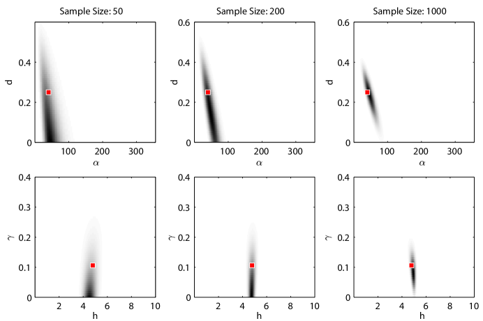
Figure 5: Convergence of $p(d,{\alpha}|{\mathbf{x}})$ for increasing sample size. Both parameterization $(d,{\alpha})$ and $(\gamma,h)$ are shown. Data are simulated from a ${\mbox{PY}}(0.25,40)$ whose parameters are indicated by the red dot.

4.2 The Pitman-Yor Mixture Entropy Estimator

Now that we have determined a prior on the infinite simplex, we turn to the problem of inference given observations ${\mathbf{x}}$. The Bayes least squares entropy estimator under the mixture prior $p(d,{\alpha})$, the Pitman-Yor Mixture (PYM) estimator, takes the form

$$\hat{H}_{\text{PYM}}=\mathbb{E}[H|{\mathbf{x}}]=\int\mathbb{E}[H|{\mathbf{x}},d,{\alpha}]\frac{p({\mathbf{x}}|d,{\alpha})p(d,{\alpha})}{p({\mathbf{x}})}\,\mathrm{d}{(d,{\alpha})},$$ (24)

where $\mathbb{E}[H|{\mathbf{x}},d,{\alpha}]$ is the expected posterior entropy for a fixed $(d,{\alpha})$ (see Section 3.2). The quantity $p({\mathbf{x}}|d,{\alpha})$ is the evidence, given by

$$p({\mathbf{x}}|d,{\alpha})=\frac{\left(\prod_{l=1}^{K-1}({\alpha}+ld)\right)\left(\prod_{i=1}^{K}\Gamma(n_{i}-d)\right)\Gamma(1+{\alpha})}{\Gamma(1-d)^{K}\Gamma({\alpha}+N)}.$$ (25)

We can obtain posterior credible intervals for $\hat{H}_{\text{PYM}}$ by estimating the posterior variance $\mathbb{E}[(H-\hat{H}_{\text{PYM}})^{2}|{\mathbf{x}}]$. The estimate takes the same form as (24), except that we replace $\mathbb{E}[H|{\mathbf{x}},d,{\alpha}]$ with $\operatorname*{var}[H|{\mathbf{x}},d,{\alpha}]$ in the integrand.

4.3 Computation

Due to the improperness of the prior $p(d,{\alpha})$ and the requirement of integrating over all ${\alpha}>0$ (eq. (24)), it is not obvious that the PYM estimate $\hat{H}_{\text{PYM}}$ is computationally tractable. In this section we discuss techniques for efficient and accurate computation of $\hat{H}_{\text{PYM}}$. First, we outline a compressed data representation we call the “multiplicities” representation, which substantially reduces computational cost. Then, we outline a fast method for performing the numerical integration over a suitable range of ${\alpha}$ and $d$.

4.3.1 Multiplicities

Computation of the expected entropy $\mathbb{E}[H|{\mathbf{x}},d,{\alpha}]$ can be carried out more efficiently using a representation in terms of multiplicities, a compressed statistic often used under other names (for instance the empirical histogram distribution function Paninski (2003)). Multiplicities are the number of symbols that have occurred with a given frequency in the sample. Letting $m_{k}=|\{i:n_{i}=k\}|$ denote the total number of symbols with exactly $k$ observations in the sample gives the compressed statistic ${\mathbf{m}}=\left[m_{0},m_{1},\dots,m_{M}\right]^{\top}$, where $M$ is the largest number of samples for any symbol. Note that the dot product $[0,1,\ldots,M]^{\top}{\mathbf{m}}=N$, is the total number of samples.

The multiplicities representation significantly reduces the time and space complexity of our computations for most datasets, as we need only compute sums and products involving the number symbols with distinct frequencies (at most $M$), rather than the total number of symbols $K$. In practice we compute all expressions not explicitly involving ${\bm{\pi}}$ using the multiplicities representation. For instance, in terms of the multiplicities the evidence takes the compressed form,

$$p({\mathbf{x}}|d,{\alpha})=p(m_{1},\ldots,m_{M}|d,{\alpha})$$

$$\quad=\frac{\Gamma(1+{\alpha})\prod_{l=1}^{K-1}({\alpha}+ld)}{\Gamma({\alpha}+N)}\prod_{i=1}^{M}\left(\frac{\Gamma(i-d)}{i!\Gamma(1-d)}\right)^{m_{i}}\frac{M!}{m_{i}!}.$$

4.3.2 Heuristic for Integral Computation

In principle the PYM integral over ${\alpha}$ is supported on the range $[0,\infty)$. In practice, however, the posterior is concentrated on a relatively small region of parameter space. It is generally unnecessary to consider the full integral over a semi-infinite domain. Instead, we select a subregion of $[0,1]\times[0,\infty)$ which supports the posterior up to $\epsilon$ probability mass. The posterior is unimodal in each variable $\alpha$ and $d$ separately (see Appendix D); however, we do not have a proof for the unimodality of the evidence. Nevertheless, if there are multiple modes, they must lie on a strictly decreasing line of $d$ as a function of $\alpha$ and, in practice, we find the posterior to be unimodal. We illustrate the concentration of the evidence visually in figure 5.

We compute the hessian at the MAP parameter value, $(d_{\text{MAP}},{\alpha}_{\text{MAP}})$. Using the inverse hessian as the covariance of a Gaussian approximation to the posterior, we select the grid which spans $\pm 6~{}\mathrm{std}$. We use numerical integration (Gauss-Legendre quadrature) on this region to compute the integral. When the hessian is rank-deficient (which may occur, for instance, when the ${\alpha}_{\text{MAP}}=0$ or $d_{\text{MAP}}=0$), we use Gauss-Legendre quadrature to perform the integral in $d$ over $[0,1)$, but employ a Fourier-Chebyshev numerical quadrature routine to integrate ${\alpha}$ over $[0,\infty)$ Boyd (1987).

4.4 Sampling the full posterior over $H$

The closed-form expressions for the conditional moments derived in the previous section allow us to compute PYM and its variance by 2-dimensional numerical integration. PYM’s posterior mean and variance provide essentially a Gaussian approximation to the posterior, and corresponding credible regions. However, in some situations (see Fig. 6), variance-based credible intervals are a poor approximation to the true posterior credible intervals. In these cases we may wish to examine the full posterior distribution over $H$. We describe methods for exactly sampling the posterior and argue that the posterior variance provides a good approximation to the true credible interval in most situations.

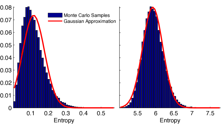
Figure 6: The posterior distributions of entropy for two datasets of $100$ samples drawn from distinct distributions and the Gaussian approximation to each distribution based upon the posterior mean and variance. (left): Simulated example with low entropy. Notice that the true posterior is highly asymmetric, and that the Gaussian approximation does not respect the positivity of $H$. (right) Simulated example with higher entropy. The Gaussian approximation is a much closer approximation to the true distribution.

Stick-breaking, as described by (14), provides a straightforward algorithm for sampling distributions ${\bm{\pi}}\sim{\mbox{PY}}(d,{\alpha})$. With large enough $N_{s}$, stick-breaking samples $\left\{\tilde{\pi}_{i}\right\}_{i=1}^{N_{s}}$ approximate $\pi$ to arbitrary accuracy. Even so, sampling $\pi\sim{\mbox{PY}}(d,{\alpha})$ for $d$ near $1$, where ${\bm{\pi}}$ is likely to be heavy-tailed, may require intractably large $N_{s}$ to obtain a good approximation. We address this problem by directly estimating the entropy of the tail, ${\mbox{PY}}(d,{\alpha}+N_{s}d)$, using (17). As shown in Fig. 3, the prior variance of PY becomes arbitrarily small as for large ${\alpha}$. For sampling, $N_{s}$ need only be large enough to make the variance of the tail entropy small. The resulting sample is the entropy of the (finite) samples plus the expected entropy of the tail, $H({\bm{\pi}}^{*})+\mathbb{E}[H|d,{\alpha}+Kd]$.

Sampling entropy is most useful for very small amounts of data drawn from distributions with low expected entropy. In Fig. 5 we illustrate the posterior distributions of entropy in two simulated experiments. In general, as the expected entropy and sample size increase, the posterior becomes more approximately Gaussian.

5 Theoretical properties of PYM

Having defined PYM and discussed its practical computation, we now establish conditions under which (24) is defined (that is, the right–hand of the equation is finite), and also prove some basic facts about its asymptotic properties. While $\hat{H}_{\text{PYM}}$ is a Bayesian estimator, we wish to build connection to the literature by showing frequentist properties.

Note that the prior expectation $\mathbb{E}[H]$ does not exist for the improper prior defined above, since $p(h=\mathbb{E}[H])\propto 1$ on $[0,\infty]$. It is therefore reasonable to ask what conditions on the data are sufficient to obtain finite posterior expectation $\hat{H}_{\text{PYM}}=E[H|{\mathbf{x}}]$. We give an answer to this question in the following short proposition (proofs of all statements may be found in the appendix),

Theorem 2

Given a fixed dataset ${\mathbf{x}}$ of $N$ samples, $\hat{H}_{\text{PYM}}<\infty$ for any prior distribution $p(d,{\alpha})$ if $N-K\geq 2$.

In other words, we require $2$ coincidences in the data for $\hat{H}_{\text{PYM}}$ to be finite. When no coincidences have occurred in ${\mathbf{x}}$, we have no evidence regarding the support of the ${\bm{\pi}}$, and our resulting entropy estimate is unbounded. In fact, in the absence of coincidences, no entropy estimator can give a reasonable estimate without prior knowledge or assumptions about $\mathcal{A}$.

Concerns about inadequate numbers of coincidences are peculiar to the undersampled regime; as $N\to\infty$, we will almost surely observe each letter infinitely often. We now turn to asymptotic considerations, establishing consistency of $\hat{H}_{\text{PYM}}$ in the limit of large $N$ for a broad class of distributions. It is known that the plugin is consistent for any distribution (finite or countably infinite), although the rate of convergence can be arbitrarily slow Antos and Kontoyiannis (2001). Therefore, we establish consistency by showing asymptotic convergence to the plugin estimator.

For clarity, we explicitly denote a quantity’s dependence upon sample size $N$ by introducing a subscript. Thus, ${\mathbf{x}}$ and $K$ become ${\mathbf{x}}_{N}$ and $K_{N}$, respectively. As a first step, we show that $\mathbb{E}[H|{\mathbf{x}}_{N},d,{\alpha}]$ converges to the plugin estimator.

Theorem 3

Assuming ${\mathbf{x}}_{N}$ drawn from a fixed, finite or countably infinite discrete distribution ${\bm{\pi}}$ such that $\frac{K_{N}}{N}\xrightarrow{P}0$,

$$\left|\mathbb{E}[H|{\mathbf{x}}_{N},d,{\alpha}]-\mathbb{E}[H_{\mathrm{plugin}}|{\mathbf{x}}_{N}]\right|\xrightarrow{P}0$$

The assumption $K_{N}/N\to 0$ is more general than it may seem. For any infinite discrete distribution, it holds that $K_{N}\to\mathbb{E}[K_{N}]$ a.s., and $\mathbb{E}[K_{N}]/N\to 0$ a.s. Gnedin et al. (2007), and so $K_{N}/N\to 0$ in probability for an arbitrary distribution. As a result, the right–hand–side of (20) shares its asymptotic behavior with $\hat{H}_{\text{plugin}}$, in particular consistency. As (20) is consistent for each value of ${\alpha}$ and $d$, it is intuitively plausible that $\hat{H}_{\text{PYM}}$, as a mixture of such values, should be consistent as well. However, while (20) alone is well-behaved, it is not clear that $\hat{H}_{\text{PYM}}$ should be. Since $\mathbb{E}[H|{\mathbf{x}},d,{\alpha}]\to\infty$ as ${\alpha}\to\infty$, care must be taken when integrating over $p(d,{\alpha}|{\mathbf{x}})$. Our main consistency result is,

Theorem 4

For any proper prior or bounded improper prior $p(d,{\alpha})$, if data ${\mathbf{x}}_{N}$ are drawn from a fixed, countably infinite discrete distribution ${\bm{\pi}}$ such that for some constant $C>0$, $K_{N}=o(N^{1-1/C})$ in probability, then

$$|\mathbb{E}[H|{\mathbf{x}}_{N}]-\mathbb{E}[H_{\mathrm{plugin}}|{\mathbf{x}}_{N}]|\xrightarrow{P}0$$

Intuitively, the asymptotic behavior of $K_{N}/N$ is tightly related to the tail behavior of the distribution Gnedin et al. (2007). In particular, $K_{N}\sim cN^{b}$ with $0<b<1$ if and only if $\pi_{i}\sim c^{\prime}i^{\frac{1}{b}}$ where $c$ and $c^{\prime}$ are constants, and we assume $\pi_{i}$ is non-increasing Gnedin et al. (2007). The class of distributions such that $K_{N}=o(N^{1-1/C})$ a.s. includes the class of power-law or thinner tailed distributions, i.e., $\pi_{i}=O(i^{b})$ for some $b>1$ (again $\pi_{i}$ is assumed non-increasing).

We conclude this section with some remarks on the role of the prior in Theorem 4 as well as the significance of asymptotic results in general. While consistency is an important property for any estimator, we emphasize that PYM is designed to address the undersampled regime. Indeed, since $\hat{H}_{\text{plugin}}$ is consistent and has an optimal rate of convergence for a large class of distributions Vu et al. (2007); Antos and Kontoyiannis (2001); Zhang (2012), asymptotic properties provide little reason to use $\hat{H}_{\text{PYM}}$. Nevertheless, notice that Theorem 4 makes very weak assumptions about $p(d,{\alpha})$. In particular, the result is not dependent upon the form of the PYM prior introduced in the previous section: it holds for any probability distribution $p(d,{\alpha})$, or even a bounded improper prior. Thus, we can view Theorem 4 as a statement about a class of PYM estimators. Almost any prior we choose on $(d,{\alpha})$ results in a consistent estimator of entropy.

6 Simulation Results

We compare $\hat{H}_{\text{PYM}}$ to other proposed entropy estimators using several example datasets. Each plot in Figs 7, 8, 9, and 10 shows convergence as well as small sample performance. We compare our estimators, DPM ($d=0$ only) and PYM ($\hat{H}_{\text{PYM}}$), with other enumerable-support estimators: coverage-adjusted estimator (CAE) Chao and Shen (2003); Vu et al. (2007), asymptotic NSB (ANSB, section 2.4) Nemenman (2011), Grassberger’s asymptotic bias correction (GR08) Grassberger (2008), and Good-Turing estimator Zhang (2012). Note that similar to ANSB, DPM is an asymptotic (Poisson-Dirichlet) limit of NSB, and hence in practice behaves identically to NSB with large but finite $K$. We also compare with plugin (3) and a standard Miller-Maddow (MiMa) bias correction method with a conservative assumption that the number of uniquely observed symbols is $K$ Miller (1955). To make comparisons more straightforward, we do not apply additional bias correction methods (e.g. jackknife) to any of the estimators.

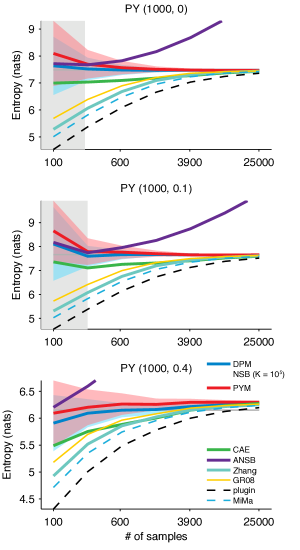
Figure 7: Comparison of estimators on stick-breaking distributions. Poisson-Dirichlet distribution with $(d=0,{\alpha}=1000)$ (top), $(d=0.1,{\alpha}=1000)$ (middle), $(d=0.4,{\alpha}=100)$ (bottom). Recall that the Dirichlet Process is the Pitman-Yor Process with $d=0$. We compare our estimators (DPM, PYM) with other enumerable support estimators (CAE, ANSB, Zhang, GR08), and finite support estimators (plugin, MiMa). Note that in these examples, the DPM estimator performs indistinguishably from NSB with alphabet size $\mathcal{A}$ is fixed to a large value ($\mathcal{A}=10^{5}$). For the experiments, we first sample a single ${\bm{\pi}}\sim{\mbox{PY}}(d,{\alpha})$ using the stick-breaking procedure of (14). For each $N$ ($x$-axis), we apply all estimators to each of 10 sample datasets drawn randomly from ${\bm{\pi}}$. Solid lines are averages over all 10 realizations. Colored shaded area represent $95\%$ credible intervals averaged over all 10 realizations. Gray shaded area represents the ANSB approximation regime defined as expected number of unique symbols being more than 90% the total number of samples.

In each simulation, we draw 10 sample distributions ${\bm{\pi}}$. From each ${\bm{\pi}}$ we draw a dataset of N iid samples. In each figure we show the performance of all estimators averaged across the 10 sampled datasets.

The experiments of Fig. 7 show performance on a single ${\bm{\pi}}\sim{\mbox{PY}}(d,{\alpha})$ drawn using the stick-breaking procedure of (14). We draw $\pi_{i}$ according to (14) in blocks of size $10^{3}$ until $1-\sum_{N_{s}}\pi_{i}<10^{-3}$, where $N_{s}$ is the number of sticks. Unsurprisingly, PYM performs well when the data are truly generated by a Pitman-Yor process (Fig. 7). Credible intervals for DPM tend to be smaller than PYM, although both shrink quickly (indicating high confidence). When the tail of the distribution is exponentially decaying, ($d=0$ case; Fig. 7 top), DPM shows slightly improved performance. When the tail has a strong power-law decay, (Fig. 7 bottom), PYM performs better than DPM. Most of the other estimators are consistently biased down, with the exception of ANSB.

The shaded gray area indicates the ANSB approximation regime, where the approximation used to define the ANSB estimator is approximately valid. Although this region has no definitive boundary, it corresponds to a regime where where the average number of coincidences is small relative to the number of samples. Following Nemenman (2011), we define the undersampled regime to be the region where $E[K_{N}]/N>0.9$, where $K_{N}$ is the number of unique symbols appearing in a sample of size $N$. Note that only 3 out of 10 results in Figs. 7,8,9,10 have shaded area; the ANSB approximation regime is not large enough to appear in the plots. This regime appears to be designed for a relatively broad distribution (close to uniform distribution). In cases where a single symbol has high probability, the ANSB approximation regime is essentially never valid. In our example distributions, this is the case with for power-law distributions and $\mathcal{PY}$ distributions with large $d$. For example, Fig. 8 is already outside of the ANSB approximation regime with only 4 samples.

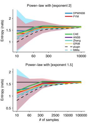
Figure 8: Comparison of estimators on power-law distributions. The highest probabilities in those power-law distributions were big enough such that they were never effectively undersampled.

Although Pitman-Yor process ${\mbox{PY}}(d,{\alpha})$ has a power-law tail controlled by $d$, the high probability portion is modulated by ${\alpha}$, and does not strictly follow a power-law distribution as a whole. In Fig. 8, we evaluate the performance for $p_{i}\propto i^{-2}$ and $p_{i}\propto i^{-1.5}$. PYM and DPM has slight negative bias, but the credible interval covers the true entropy for all sample sizes. For small sample sizes, most estimators are negatively biased, again except for ANSB (which does not show up in the plot since it is severely biased upwards). Notably CAE performs very well in moderate sample sizes.

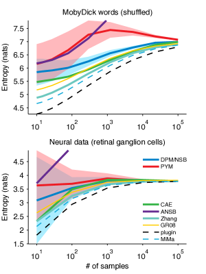
Figure 9: Comparison of estimators on real data sets.

In Fig. 9, we compute the entropy per word of in the novel Moby Dick by Herman Melville, and entropy per time bin of a population of retinal ganglion cells from monkey retina Pillow et al. (2005). We tokenized the novel into individual words using the Python library NLTK. Punctuation is disregarded. These real-world datasets have heavy, approximately power-law tails as pointed out earlier in Fig. 2. For Moby Dick, PYM slightly overestimates, while DPM slightly underestimates, yet both methods are closer to the entropy estimated by the full data available than other estimators. DPM is overly confident (its credible interval is too narrow), while PYM becomes overly confident with more data. The neural data were preprocessed to be a binarized response (10 ms time bins) of 8 simultaneously recorded off-response retinal ganglion cells. PYM, DPM, and CAE all perform well on this dataset, with both PYM and DPM bracketing the asymptotic value with their credible intervals.

Finally, we applied the denumerable support estimators to finite support distributions (Fig. 10). The power-law $p_{n}\propto n^{-1}$ has the heaviest tail among the simulations we consider, but notice that it does not define a proper distribution (the probability mass does not integrate), and so we use a truncated $1/n$ distribution with the first $1000$ symbols (Fig. 10 top). Initially PYM shows the least bias, but DPM provides a better estimate for increasing sample size. Notice, however, that for both estimates the credible intervals consistently cover the true entropy. Interestingly, the finite support estimators perform poorly compared to DPM, CAE and PYM. For the uniform distribution over $1000$ symbols, both DPM and PYM have slight upward bias, while CAE shows almost perfect performance (Fig. 10 middle). For Poisson distribution, a theoretically enumerable-support distribution on the natural numbers, the tail decays so quickly that the effective support (due to machine precision) is very small ($26$ in this case). All the estimators, with the exception of ANSB, work quite well. The novel Moby Dick provides the most challenging data: no estimator seems to have converged, even with the full data. Surprisingly, the Good-Turing estimator Zhang (2012) tends to perform similarly to the Grassberger and Miller-Maddow bias-correction methods. Among such the bias-correction methods, Grassberger’s method tended to show the best performance, outperforming Zhang’s method.

The computation time for our estimators is $O(LG)$, where $L$ number symbols with distinct frequencies (bounded above by the quantity $M$ defined in Section 4.3.1) and $G$ is the number of gridpoints used to compute the numerical integral. Hence, computation time as a function of sample size depends upon how $L$ scales with samples size $N$, always sublinearly, and $O(N^{1/2})$ in the worse case. In our examples, computation times for $10^{5}$ samples are in the order of 0.1 seconds (Fig. 11). Hence in practice, for the examples we have shown, more time is spent building the histogram from the data than computing the entropy estimate.

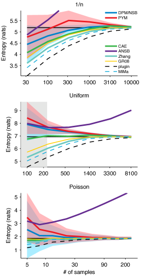
Figure 10: Comparison of estimators on finite support distributions. Black solid line indicates the true entropy. Poisson distribution ($\lambda=e$) has a countably infinite tail, but a very thin one—all probability mass was concentrated in 26 symbols within machine precision.

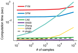
Figure 11: Median computation time to estimate entropy for the neural data. The computation time excludes the preprocessing required to build the histogram and convert to multiplicity representation. Note that for DPM and PYM this time also includes estimating the posterior variance.

7 Conclusion

In this paper we introduced PYM, a new entropy estimator for distributions with unknown support. We derived analytic forms for the conditional mean and variance of entropy under a DP and PY prior for fixed parameters. Inspired by the work of Nemenman et al. (2002), we defined a novel PY mixture prior, PYM, which implies an approximately flat prior on entropy. PYM addresses two major issues with NSB: its dependence on knowledge of $\mathcal{A}$ and its inability (inherited from the Dirichlet distribution) to account for the heavy-tailed distributions which abound in biological and other natural data.

Futher experiments on diverse datasets might reveal ways to improve PYM, such as new tactics or theory for selecting the prior on tail behavior, $q(\gamma)$. It may also prove fruitful to investigate ways to tailor PYM to a specific application, for instance by combining it with with more structured priors, such as those employed in Archer et al. (2013). Further, while we have shown that PYM is consistent for any prior, an expanded theory might investigate the convergence rate, perhaps in relation to the choice of prior.

We have shown that PYM performs well in comparison to other entropy estimators, and indicated its practicality in example applications to data. A MATLAB implementation of the PYM estimator is available at https://github.com/pillowlab/PYMentropy.

A Derivations of Dirichlet and PY moments

In this Appendix we present as propositions a number of technical moment derivations used in the text.

A.1 Mean entropy of finite Dirichlet

Proposition 5 (Replica trick for entropy Wolpert and Wolf (1995))

For ${\bm{\pi}}\sim\mathrm{Dir}(\alpha_{1},\alpha_{2},\dots,\alpha_{\mathcal{A}})$, such that $\sum_{i=1}^{\mathcal{A}}\alpha_{i}=A$, and letting $\vec{\alpha}=\left(\alpha_{1},\alpha_{2},\dots,\alpha_{\mathcal{A}}\right)$, we have

$$\mathbb{E}[H({\bm{\pi}})|\vec{\alpha}] = \psi_{0}(A+1)-\sum_{i=1}^{\mathcal{A}}\frac{\alpha_{i}}{A}\psi_{0}(\alpha_{i}+1)$$ (26)

Proof  First, let $c$ be the normalizer of Dirichlet, $c=\frac{\prod_{j}\Gamma(\alpha_{j})}{\Gamma(A)}$ and let $\mathcal{L}$ denote the Laplace transform (on $\pi$ to $s$). Now,

$$c\mathbb{E}[H|\vec{\alpha}] =\int\left(-\sum_{i}\pi_{i}\log_{2}\pi_{i}\right)\delta({\scriptstyle\sum_{i}}\pi_{i}-1)\prod_{j}\pi_{j}^{\alpha_{j}-1}d{\bm{\pi}}$$

$$=-\sum_{i}\int\left(\pi_{i}^{\alpha_{i}}\log_{2}\pi_{i}\right)\delta({\scriptstyle\sum_{i}}\pi_{i}-1)\prod_{j\neq i}\pi_{j}^{\alpha_{j}-1}d{\bm{\pi}}$$

$$=-\sum_{i}\int\left(\frac{d}{d(\alpha_{i})}\pi_{i}^{\alpha_{i}}\right)\delta({\scriptstyle\sum_{i}}\pi_{i}-1)\prod_{j\neq i}\pi_{j}^{\alpha_{j}-1}d{\bm{\pi}}$$

$$=-\sum_{i}\frac{d}{d(\alpha_{i})}\int\pi_{i}^{\alpha_{i}}\delta({\scriptstyle\sum_{i}}\pi_{i}-1)\prod_{j\neq i}\pi_{j}^{\alpha_{j}-1}d{\bm{\pi}}$$

$$=-\sum_{i}\frac{d}{d(\alpha_{i})}\mathcal{L}^{-1}\left[\mathcal{L}(\pi_{i}^{\alpha_{i}})\prod_{j\neq i}\mathcal{L}(\pi_{j}^{\alpha_{j}-1})\right](1)$$

$$=-\sum_{i}\frac{d}{d(\alpha_{i})}\mathcal{L}^{-1}\left[\frac{\Gamma(\alpha_{i}+1)\prod_{j\neq i}\Gamma({\alpha_{j}})}{s^{\sum_{k}(\alpha_{k})+1}}\right](1)$$

$$=-\sum_{i}\frac{d}{d(\alpha_{i})}\left[\frac{\Gamma(\alpha_{i}+1)}{\Gamma(\sum_{k}(\alpha_{k})+1)}\right]\prod_{j\neq i}\Gamma({\alpha_{j}})$$

$$=-\sum_{i}\frac{\Gamma(\alpha_{i}+1)}{\Gamma(\sum_{k}\alpha_{k}+1)}\left[\psi_{0}(\alpha_{i}+1)-\psi_{0}(A+1)\right]\prod_{j\neq i}\Gamma({\alpha_{j}})$$

$$=\left[\psi_{0}(A+1)-\sum_{i=1}^{\mathcal{A}}\frac{\alpha_{i}}{A}\psi_{0}(\alpha_{i}+1)\right]\frac{\prod_{j}\Gamma({\alpha_{j}})}{\Gamma(A)}.$$

 

A.2 Variance entropy of finite Dirichlet

We derive $\mathbb{E}[H^{2}({\bm{\pi}})|\vec{\alpha}]$. In practice we compute $\operatorname*{var}[H({\bm{\pi}})|\vec{\alpha}]=\mathbb{E}[H^{2}({\bm{\pi}})|\vec{\alpha}]-\mathbb{E}[H({\bm{\pi}})|\vec{\alpha}]^{2}$.

Proposition 6

For ${\bm{\pi}}\sim\mathrm{Dir}(\alpha_{1},\alpha_{2},\dots,\alpha_{\mathcal{A}})$, such that $\sum_{i=1}^{\mathcal{A}}\alpha_{i}=A$, and letting $\vec{\alpha}=\left(\alpha_{1},\alpha_{2},\dots,\alpha_{\mathcal{A}}\right)$, we have

$$\mathbb{E}[H^{2}({\bm{\pi}})|\vec{\alpha}] =\sum_{i\neq k}\frac{\alpha_{i}\alpha_{k}}{(A+1)(A)}I_{ik}+\sum_{i}\frac{\alpha_{i}(\alpha_{i}+1)}{(A+1)(A)}J_{i}$$ (27)

$$I_{ik} =\left(\psi_{0}(\alpha_{k}+1)-\psi_{0}(A+2)\right)\left(\psi_{0}(\alpha_{i}+1)\right.$$

$$\qquad\left.-\psi_{0}(A+2)\right)-\psi_{1}(A+2)$$

$$J_{i} =(\psi_{0}(\alpha_{i}+2)-\psi_{0}(A+2))^{2}+\psi_{1}(\alpha_{i}+2)$$

$$\qquad-\psi_{1}(A+2)$$

Proof  We can evaluate the second moment in a manner similar to the mean entropy above. First, we split the second moment into square and cross terms. To evaluate the integral over the cross terms, we apply the “replica trick” twice. Letting $c$ be the normalizer of Dirichlet, $c=\frac{\prod_{j}\Gamma(\alpha_{j})}{\Gamma(A)}$ we have,

$$c\mathbb{E}[H^{2}|\vec{\alpha}]=\int\left(-\sum_{i}\pi_{i}\log_{2}\pi_{i}\right)^{2}\delta({\scriptstyle\sum_{i}}\pi_{i}-1)\prod_{j}\pi_{j}^{\alpha_{j}-1}d{\bm{\pi}}$$

$$=\sum_{i}\int\left(\pi_{i}^{2}{\log_{2}}^{2}\pi_{i}\right)\delta({\scriptstyle\sum_{i}}\pi_{i}-1)\prod_{j}\pi_{j}^{\alpha_{j}-1}d{\bm{\pi}}$$

$$+\sum_{i\neq k}\int\left(\pi_{i}\log_{2}\pi_{i}\right)\left(\pi_{k}\log_{2}\pi_{k}\right)\delta({\scriptstyle\sum_{i}}\pi_{i}-1)\prod_{j}\pi_{j}^{\alpha_{j}-1}d{\bm{\pi}}$$

$$=\sum_{i}\int\pi_{i}^{\alpha_{i}+1}{\log_{2}}^{2}\pi_{i}\delta({\scriptstyle\sum_{i}}\pi_{i}-1)\prod_{j\neq i}\pi_{j}^{\alpha_{j}-1}d{\bm{\pi}}$$

$$+\sum_{i\neq k}\int\left(\pi_{i}^{\alpha_{i}}\log_{2}\pi_{i}\right)\left(\pi_{k}^{\alpha_{k}}\log_{2}\pi_{k}\right)\delta({\scriptstyle\sum_{i}}\pi_{i}-1)\prod_{j\not\in\{i,k\}}\pi_{j}^{\alpha_{j}-1}d{\bm{\pi}}$$

$$=\sum_{i}\frac{d^{2}}{d(\alpha_{i}+1)^{2}}\int\pi_{i}^{\alpha_{i}+1}\delta({\scriptstyle\sum_{i}}\pi_{i}-1)\prod_{j\neq i}\pi_{j}^{\alpha_{j}-1}d{\bm{\pi}}$$

$$+\sum_{i\neq k}\frac{d}{d\alpha_{i}}\frac{d}{d\alpha_{k}}\int\left(\pi_{i}^{\alpha_{i}}\right)\left(\pi_{k}^{\alpha_{k}}\right)\delta({\scriptstyle\sum_{i}}\pi_{i}-1)\prod_{j\not\in\{i,k\}}\pi_{j}^{\alpha_{j}-1}d{\bm{\pi}}$$

Assuming $i\neq k$, these will be the cross terms.

$$\int(\pi_{i}\log_{2}\pi_{i})(\pi_{k}\log_{2}\pi_{k})\delta({\scriptstyle\sum_{i}}\pi_{i}-1)\prod_{j}\pi_{j}^{\alpha_{j}-1}d{\bm{\pi}}$$

$$=\frac{d}{d\alpha_{i}}\frac{d}{d\alpha_{k}}\int(\pi_{i}^{\alpha_{i}})(\pi_{k}^{\alpha_{k}})\delta({\scriptstyle\sum_{i}}\pi_{i}-1)\prod_{j\not\in\{i,k\}}\pi_{j}^{\alpha_{j}-1}d{\bm{\pi}}$$

$$=\frac{d}{d\alpha_{i}}\frac{d}{d\alpha_{k}}\left[\frac{\Gamma(\alpha_{i}+1)\Gamma(\alpha_{k}+1)}{\Gamma(A+2)}\right]\prod_{j\not\in\{i,k\}}\Gamma({\alpha_{j}})$$

$$=\frac{d}{d\alpha_{k}}\left[\frac{\alpha_{i}\Gamma(\alpha_{k}+1)}{\Gamma(A+2)}\psi_{0}(\alpha_{i}+1)\right.$$

$$\qquad\qquad\left.-\frac{\alpha_{i}\Gamma(\alpha_{k}+1)}{\Gamma(A+2)}\psi_{0}(A+2)\right]\prod_{j\neq k}\Gamma({\alpha_{j}})$$

$$=\frac{d}{d\alpha_{k}}\left[\frac{\alpha_{i}\psi_{0}(\alpha_{k}+1)}{\Gamma(A+2)}\psi_{0}(\alpha_{i}+1)\right.$$

$$\qquad\qquad\left.-\frac{\alpha_{i}\Gamma(\alpha_{k}+1)}{\Gamma(A+2)}\psi_{0}(A+2)\right]\prod_{j\neq k}\Gamma({\alpha_{j}})$$

$$=\frac{\alpha_{i}\alpha_{k}}{\Gamma(A+2)}\left[(\psi_{0}(\alpha_{k}+1)-\psi_{0}(A+2))\right.$$

$$\qquad\left.(\psi_{0}(\alpha_{i}+1)-\psi_{0}(A+2))-\psi_{1}(A+2)\right]\prod_{j}\Gamma({\alpha_{j}})$$

$$=\frac{\alpha_{i}\alpha_{k}}{(A+1)(A)}\left[\left(\psi_{0}(\alpha_{k}+1)-\psi_{0}(A+2)\right)\right.$$

$$\qquad\left.\left(\psi_{0}(\alpha_{i}+1)-\psi_{0}(A+2)\right)-\psi_{1}(A+2)\right]\frac{\prod_{j}\Gamma({\alpha_{j}})}{\Gamma(A)}$$

$$\frac{d^{2}}{d(\alpha_{i}+1)^{2}}\int\pi_{i}^{\alpha_{i}+1}\delta({\scriptstyle\sum_{i}}\pi_{i}-1)\prod_{j\neq i}\pi_{j}^{\alpha_{j}-1}d{\bm{\pi}}$$

$$=\frac{d^{2}}{d(\alpha_{i}+1)^{2}}\left[\frac{\Gamma(\alpha_{i}+2)}{\Gamma(A+2)}\right]\prod_{j\neq i}\Gamma({\alpha_{j}})$$

$$=\frac{d^{2}}{dz^{2}}\left[\frac{\Gamma(z+1)}{\Gamma(z+c)}\right]\prod_{j\neq i}\Gamma({\alpha_{j}}),~{}~{}~{}\left\{c=A+2-(\alpha_{i}+1)\right\}$$

$$=\frac{\Gamma(1+z)}{\Gamma(c+z)}\left[(\psi_{0}(1+z)-\right.$$

$$\qquad\left.\psi_{0}(c+z))^{2}+\psi_{1}(1+z)-\psi_{1}(c+z)\right]\prod_{j\neq i}\Gamma({\alpha_{j}})$$

$$=\frac{z(z-1)}{(c+z-1)(c+z-2)}\left[(\psi_{0}(1+z)-\psi_{0}(c+z))^{2}\right.$$

$$\qquad\qquad\qquad\left.+\psi_{1}(1+z)-\psi_{1}(c+z)\right]\frac{\prod_{j}\Gamma({\alpha_{j}})}{\Gamma(A)}$$

$$=\frac{(\alpha_{i}+1)(\alpha_{i})}{(A+1)(A)}\left[(\psi_{0}(\alpha_{i}+2)-\psi_{0}(A+2))^{2}+\psi_{1}(\alpha_{i}+2)\right.$$

$$\qquad\qquad\qquad\left.-\psi_{1}(A+2)\right]\frac{\prod_{j}\Gamma({\alpha_{j}})}{\Gamma(A)}$$

Summing over all terms and adding the cross and square terms, we recover the desired expression for $\mathbb{E}[H^{2}({\bm{\pi}})|\vec{\alpha}]$.  

A.3 Prior entropy mean and variance under PY

We derive the prior entropy mean and variance of a PY distribution with fixed parameters $\alpha$ and $d$, $\mathbb{E}_{\bm{\pi}}[H({\bm{\pi}})|d,\alpha]$ and $\operatorname*{var}{\bm{\pi}}[H({\bm{\pi}})|d,\alpha]$. We first prove our Proposition 1 (mentioned in Pitman and Yor (1997)). This proposition establishes the identity $\mathbb{E}\left[\sum_{i=1}^{\infty}f(\pi_{i})\Big{|}\alpha\right]=\int_{0}^{1}\frac{f(\tilde{\pi}_{1})}{\tilde{\pi}_{1}}p(\tilde{\pi}_{1}|\alpha)d\tilde{\pi}_{1}$ which will allow us to compute expectations over PY using only the distribution of the first size biased sample, $\tilde{\pi}_{1}$.

Proof [Proof of Proposition 1]

First we validate (15). Writing out the general form of the size-biased sample,

$$p(\tilde{\pi}_{1}=x|{\bm{\pi}})=\sum_{i=1}^{\infty}\pi_{i}\delta(x-\pi_{i}),$$

we see that

$$\mathbb{E}_{\tilde{\pi}_{1}}\left[\frac{f(\tilde{\pi}_{1})}{\tilde{\pi}_{1}}\right] =\int_{0}^{1}\frac{f(x)}{x}p(\tilde{\pi}_{1}=x)dx$$

$$=\int_{0}^{1}\mathbb{E}_{\bm{\pi}}\left[\frac{f(x)}{x}p(\tilde{\pi}_{1}=x|{\bm{\pi}})\right]dx$$

$$=\int_{0}^{1}\mathbb{E}_{\bm{\pi}}\left[\sum_{i=1}^{\infty}\frac{f(x)}{x}\pi_{i}\delta(x-\pi_{i})\right]dx$$

$$=\mathbb{E}_{\bm{\pi}}\left[\int_{0}^{1}\sum_{i=1}^{\infty}\frac{f(x)}{x}\pi_{i}\delta(x-\pi_{i})dx\right]$$

$$=\mathbb{E}_{\bm{\pi}}\left[\sum_{i=1}^{\infty}\int_{0}^{1}\frac{f(x)}{x}\pi_{i}\delta(x-\pi_{i})dx\right]$$

$$=\mathbb{E}_{\bm{\pi}}\left[\sum_{i=1}^{\infty}f(\pi_{i})\right],$$

where the interchange of sums and integrals is justified by Fubini’s theorem.

A similar method validates (16). We will need the second size-biased sample in addition to the first. We begin with the sum inside the expectation on the left–hand side of (16),

$$\sum_{i}\sum_{j\neq i}g(\pi_{i},\pi_{j})$$ (28)

$$=\frac{\sum_{i}\sum_{j\neq i}g(\pi_{i},\pi_{j})}{p(\tilde{\pi}_{1}=\pi_{i},\tilde{\pi}_{2}=\pi_{j})}p(\tilde{\pi}_{1}=\pi_{i},\tilde{\pi}_{2}=\pi_{j})$$ (29)

$$=\sum_{i}\sum_{j\neq i}\frac{g(\pi_{i},\pi_{j})}{\pi_{i}\pi_{j}}(1-\pi_{i})p(\tilde{\pi}_{1}=\pi_{i},\tilde{\pi}_{2}=\pi_{j})$$ (30)

$$=\mathbb{E}_{\tilde{\pi}_{1},\tilde{\pi}_{2}}\left[\frac{g(\tilde{\pi}_{1},\tilde{\pi}_{2})}{\tilde{\pi}_{1}\tilde{\pi}_{2}}(1-\tilde{\pi}_{1})\Big{|}{\bm{\pi}}\right]$$ (31)

where the joint distribution of size biased samples is given by,

$$p(\tilde{\pi}_{1}=\pi_{i},\tilde{\pi}_{2}=\pi_{j}) =p(\tilde{\pi}_{1}=\pi_{i})p(\tilde{\pi}_{2}=\pi_{j}|\tilde{\pi}_{1}=\pi_{i})$$

$$=\pi_{i}\cdot\frac{\pi_{j}}{1-\pi_{i}}.$$

 

As this identity is defined for any additive functional $f$ of ${\bm{\pi}}$; we can employ it to compute the first two moments of entropy. For PYP (and DP when $d=0$), the first size-biased sample is distributed according to:

$$\tilde{\pi}_{1}\sim\mathrm{Beta}(1-d,\alpha+d)$$ (32)

Proposition 1 gives the mean entropy directly. Taking $f(x)=-x\log(x)$ we have,

$$\mathbb{E}[H({\bm{\pi}})|d,\alpha]=-\mathbb{E}_{\alpha}[\log(\pi_{1})]=\psi_{0}(\alpha+1)-\psi_{0}(1-d),$$

The same method may be used to obtain the prior variance, although the computation is more involved. For the variance, we will need the second size-biased sample in addition to the first. The second size-biased sample is given by,

$$\tilde{\pi}_{2}=(1-\tilde{\pi}_{1})v_{2},\quad v_{2}\sim\mathrm{Beta}(1-d,\alpha+2d)$$ (33)

We will compute the second moment explicitly, splitting $H({\bm{\pi}})^{2}$ into square and cross terms,

$$\mathbb{E}[\left(H({\bm{\pi}})\right)^{2}|d,\alpha] =\mathbb{E}\left[\left.\left(-\sum_{i}\pi_{i}\log(\pi_{i})\right)^{2}\right|d,\alpha\right]$$

$$=\mathbb{E}\left[\left.\sum_{i}\left(\pi_{i}\log(\pi_{i})\right)^{2}\right|d,\alpha\right]$$ (34)

$$+\mathbb{E}\left[\left.\sum_{i}\sum_{j\neq i}\pi_{i}\pi_{j}\log(\pi_{i})\log(\pi_{j})\right|d,\alpha\right]$$ (35)

The first term follows directly from (15),

$$\mathbb{E}\left[\left.\sum_{i}\left(\pi_{i}\log(\pi_{i})\right)^{2}\right|d,\alpha\right]=\int_{0}^{1}x(-\log(x))^{2}p(x|d,\alpha)\,\mathrm{d}{x}$$

$$=B^{-1}(1-d,\alpha+d)\int_{0}^{1}x\log^{2}(x)x^{1-d}(1-x)^{\alpha+d-1}\,\mathrm{d}{x}$$

$$=\frac{1-d}{\alpha+1}\left[(\psi_{0}(2-d)-\psi_{0}(2+\alpha))^{2}+\psi_{1}(2-d)-\psi_{1}(2+\alpha)\right]$$ (36)

The second term of (35), requires the first two size biased samples, and follows from (16) with $g(x,y)=\log(x)\log(y)$. For the PYP prior, it is easier to integrate on $V_{1}$ and $V_{2}$, rather than the size biased samples. The second term is then (note that we let $\gamma=B^{-1}(1-d,\alpha+2d)$ and $\zeta=B^{-1}(1-d,\alpha+d)$),

$$\mathbb{E}\left[\mathbb{E}\left[\log(\tilde{\pi}_{1})\log(\tilde{\pi}_{2})(1-\pi_{1})|{\bm{\pi}}\right]|\alpha\right]$$

$$=\mathbb{E}\left[\mathbb{E}\left[\log(V_{1})\log((1-V_{1})V_{2})(1-V_{1})|{\bm{\pi}}\right]|\alpha\right]$$

$$=\zeta\gamma\int_{0}^{1}\int_{0}^{1}\log(v_{1})\log((1-v_{1})v_{2})(1-v_{1})v_{1}^{1-d}(1-v_{1})^{\alpha+d-1}$$

$$\qquad\qquad\qquad\qquad\times v_{2}^{1-d}(1-v_{2})^{\alpha+2d-1}\,\mathrm{d}{v_{1}}\,\mathrm{d}{v_{2}}$$

$$=\zeta\left[\int_{0}^{1}\log(v_{1})\log(1-v_{1})(1-v_{1})v_{1}^{1-d}(1-v_{1})^{\alpha+d-1}\,\mathrm{d}{v_{1}}\right.$$

$$\quad+\left.\gamma\int_{0}^{1}\log(v_{1})(1-v_{1})v_{1}^{1-d}(1-v_{1})^{\alpha+d-1}\right.$$

$$\qquad\qquad\qquad\left.\times\int_{0}^{1}\log(v_{2})v_{2}^{1-d}(1-v_{2})^{\alpha+2d-1}\,\mathrm{d}{v_{1}}\,\mathrm{d}{v_{2}}\right]$$

$$=\frac{\alpha+d}{\alpha+1}\left[(\psi_{0}(1-d)-\psi_{0}(2+\alpha))^{2}-\psi_{1}(2+\alpha)\right]$$

Finally combining the terms, the variance of the entropy under PYP prior is

$$\operatorname*{var}[H({\bm{\pi}})|d,\alpha]=$$ (37)

$$\frac{1-d}{\alpha+1}\left[(\psi_{0}(2-d)-\psi_{0}(2+\alpha))^{2}+\psi_{1}(2-d)-\psi_{1}(2+\alpha)\right]$$

$$\quad\quad+\frac{\alpha+d}{\alpha+1}\left[(\psi_{0}(1-d)-\psi_{0}(2+\alpha))^{2}-\psi_{1}(2+\alpha)\right]$$

$$\qquad-(\psi_{0}(1+\alpha)-\psi_{0}(1-d))^{2}$$

$$=\frac{\alpha+d}{(\alpha+1)^{2}(1-d)}+\frac{1-d}{\alpha+1}\psi_{1}(2-d)-\psi_{1}(2+\alpha)$$ (38)

We note that the expectations over the finite Dirichlet may also be derived using this formula by letting the $\tilde{\bm{\pi}}$ be the first size-biased sample of a finite Dirichlet on $\Delta_{\mathcal{A}}$.

A.4 Posterior Moments of PYP

First, we discuss the form of the PYP posterior, and introduce independence properties that will be important in our derivation of the mean. We recall that the PYP posterior, ${\bm{\pi}}_{\mathrm{post}}$, of (19) has three stochastically independent components: Bernoulli $p_{\ast}$, PY ${\bm{\pi}}$, and Dirichlet $\mathbf{p}$.

Component expectations: From the above derivations for expectations under the PYP and Dirichlet distributions as well as the Beta integral identities (see e.g., Archer et al. (2012)), we find expressions for $\mathbb{E}_{\mathbf{p}}\left[H(\mathbf{p})|d,\alpha\right]$, $E_{{\bm{\pi}}}\left[H({\bm{\pi}})|d,\alpha\right]$, and $\mathbb{E}_{p_{\ast}}\left[H(p_{\ast})\right]$.

$$\mathbb{E}[H({\bm{\pi}})|d,\alpha] =\psi_{0}(\alpha+1)-\psi_{0}(1-d)$$

$$\mathbb{E}_{p_{\ast}}[H(p_{\ast})] =\psi_{0}(\alpha+N+1)-\frac{\alpha+Kd}{\alpha+N}\psi_{0}(\alpha+Kd+1)$$

$$\qquad\quad-\frac{N-Kd}{\alpha+N}\psi_{0}(N-Kd+1)$$

$$\mathbb{E}_{\mathbf{p}}[H(\mathbf{p})|d,\alpha] =\psi_{0}(N-Kd+1)-\sum_{i=1}^{K}\frac{n_{i}-d}{N-Kd}\psi_{0}(n_{i}-d+1)$$

where by a slight abuse of notation we define the entropy of $p_{\ast}$ as $H(p_{\ast})=-(1-p_{\ast})\log(1-p_{\ast})-p_{\ast}\log p_{\ast}$. We use these expectations below in our computation of the final posterior integral.

Derivation of posterior mean: We now derive the analytic form of the posterior mean, (20).

$$\mathbb{E}[H(\pi_{\mathrm{post}})|d,\alpha]=\mathbb{E}\left[-\sum_{i=1}^{K}p_{i}\log{p_{i}}-p_{\ast}\sum_{i=1}^{\infty}\pi_{i}\log{p_{\ast}\pi_{i}}\Big{|}d,\alpha\right]$$

$$=\mathbb{E}\left[-(1-p_{\ast})\sum_{i=1}^{K}\frac{p_{i}}{1-p_{\ast}}\log{\left(\frac{p_{i}}{1-p_{\ast}}\right)}\right.$$

$$\quad\left.-(1-p_{\ast})\log(1-p_{\ast})-p_{\ast}\sum_{i=1}^{\infty}\pi_{i}\log{\pi_{i}}-p_{\ast}\log{p_{\ast}}\Big{|}d,\alpha\right]$$

$$=\mathbb{E}\left[-(1-p_{\ast})\sum_{i=1}^{K}\frac{p_{i}}{1-p_{\ast}}\log{\left(\frac{p_{i}}{1-p_{\ast}}\right)}\right.$$

$$\qquad\qquad\qquad\left.-p_{\ast}\sum_{i=1}^{\infty}\pi_{i}\log{\pi_{i}}+H(p_{\ast})\Big{|}d,\alpha\right]$$

$$=\mathbb{E}\left[\mathbb{E}\left[-(1-p_{\ast})\sum_{i=1}^{K}\frac{p_{i}}{1-p_{\ast}}\log{\left(\frac{p_{i}}{1-p_{\ast}}\right)}\right.\right.$$

$$\qquad\qquad\qquad\left.\left.-p_{\ast}\sum_{i=1}^{\infty}\pi_{i}\log{\pi_{i}}+H(p_{\ast})~{}\Big{|}~{}p_{\ast}\right]\Big{|}d,\alpha\right]$$

$$=\mathbb{E}\left[\mathbb{E}\left[(1-p_{\ast})H(\mathbf{p})+p_{\ast}H({\bm{\pi}})+H(p_{\ast})~{}\Big{|}~{}p_{\ast}\right]\Big{|}d,\alpha\right]$$

$$=\mathbb{E}_{p_{\ast}}\left[(1-p_{\ast})\mathbb{E}_{\mathbf{p}}\left[H(\mathbf{p})|d,\alpha\right]+p_{\ast}\mathbb{E}_{{\bm{\pi}}}\left[H({\bm{\pi}})|d,\alpha\right]+H(p_{\ast})\right]$$

using the formulae for $\mathbb{E}_{\mathbf{p}}\left[H(\mathbf{p})|d,\alpha\right]$, $\mathbb{E}_{{\bm{\pi}}}\left[H({\bm{\pi}})|d,\alpha\right]$, and $\mathbb{E}_{p_{\ast}}[H(p_{\ast})]$ and rearranging terms, we obtain (20),

$$\mathbb{E}[H(\pi_{\mathrm{post}})|d,\alpha]=\frac{A}{\alpha+N}\mathbb{E}_{\mathbf{p}}[H(\mathbf{p})]$$

$$\qquad\qquad\qquad+\frac{\alpha+Kd}{\alpha+N}\mathbb{E}_{{\bm{\pi}}}[H({\bm{\pi}})]+\mathbb{E}_{p_{\ast}}[H(p_{\ast})]$$

$$=\frac{A}{\alpha+N}\left[\psi_{0}(A+1)-\sum_{i=1}^{K}\frac{\alpha_{i}}{A}\psi_{0}(\alpha_{i}+1)\right]$$

$$\quad+\frac{\alpha+Kd}{\alpha+N}\left[\psi_{0}(\alpha+Kd+1)-\psi_{0}(1-d)\right]+$$

$$\quad\psi_{0}(\alpha+N+1)-\frac{\alpha+Kd}{\alpha+N}\psi_{0}(\alpha+Kd+1)-\frac{A}{\alpha+N}\psi_{0}(A+1)$$

$$=\psi_{0}(\alpha+N+1)-\frac{\alpha+Kd}{\alpha+N}\psi_{0}(1-d)-$$

$$\qquad\qquad\qquad\qquad\qquad\frac{A}{\alpha+N}\left[\sum_{i=1}^{K}\frac{\alpha_{i}}{A}\psi_{0}(\alpha_{i}+1)\right]$$

$$=\psi_{0}(\alpha+N+1)-\frac{\alpha+Kd}{\alpha+N}\psi_{0}(1-d)-$$

$$\qquad\qquad\qquad\qquad\qquad\frac{1}{\alpha+N}\left[\sum_{i=1}^{K}(n_{i}-d)\psi_{0}(n_{i}-d+1)\right]$$

Derivation of posterior variance: We continue the notation from the subsection above. In order to exploit the independence properties of $\pi_{\mathrm{post}}$ we first apply the law of total variance to obtain (A.4),

$$\operatorname*{var}[H(\pi_{\mathrm{post}})|d,\alpha] =\operatorname*{var}_{p_{\ast}}\left[\mathbb{E}_{{\bm{\pi}},\mathbf{p}}[H(\pi_{\mathrm{post}})]\Big{|}d,\alpha\right]$$

$$\qquad+\mathbb{E}_{p_{\ast}}\left[\operatorname*{var}_{{\bm{\pi}},\mathbf{p}}[H(\pi_{\mathrm{post}})]\Big{|}d,\alpha\right]$$ (39)

We now seek expressions for each term in (A.4) in terms of the expectations already derived.

Step 1: For the right-hand term of (A.4), we use the independence properties of $\pi_{\mathrm{post}}$ to express the variance in terms of PYP, Dirichlet, and Beta variances,

$$\mathbb{E}_{p_{\ast}}\left[\operatorname*{var}_{{\bm{\pi}},\mathbf{p}}[H(\pi_{\mathrm{post}})|p_{\ast}]\Big{|}d,\alpha\right]$$ (40)

$$=\mathbb{E}_{p_{\ast}}\left[(1-p_{\ast})^{2}\operatorname*{var}_{\mathbf{p}}[H(\mathbf{p})]+p_{\ast}^{2}\operatorname*{var}_{{\bm{\pi}}}[H({\bm{\pi}})]\Big{|}d,\alpha\right]$$

$$=\frac{(N-Kd)(N-Kd+1)}{(\alpha+N)(\alpha+N+1)}\operatorname*{var}_{\mathbf{p}}[H(\mathbf{p})]$$

$$\qquad\qquad+\frac{(\alpha+Kd)(\alpha+Kd+1)}{(\alpha+N)(\alpha+N+1)}\operatorname*{var}_{{\bm{\pi}}}[H({\bm{\pi}})]$$ (41)

Step 2: In the left-hand term of (A.4) the variance is with respect to the $\mathrm{Beta}$ distribution, while the inner expectation is precisely the posterior mean we derived above. Expanding, we obtain,

$$\operatorname*{var}_{p_{\ast}}\left[\mathbb{E}_{{\bm{\pi}},\mathbf{p}}[H(\pi_{\mathrm{post}})|p_{\ast}]\Big{|}d,\alpha\right]$$

$$=\operatorname*{var}_{p_{\ast}}\left[(1-p_{\ast})\mathbb{E}_{\mathbf{p}}\left[H(\mathbf{p})\right]+p_{\ast}\mathbb{E}_{{\bm{\pi}}}\left[H({\bm{\pi}})|p_{\ast}\right]+H(p_{\ast})\Big{|}d,\alpha\right]$$ (42)

To evaluate this integral, we introduce some new notation,

$$\mathbf{A} =\mathbb{E}_{\mathbf{p}}\left[H(\mathbf{p})\right]$$

$$\mathbf{B} =\mathbb{E}_{{\bm{\pi}}}\left[H({\bm{\pi}})\right]$$

$$\Omega(p_{\ast}) =(1-p_{\ast})\mathbb{E}_{\mathbf{p}}\left[H(\mathbf{p})\right]+p_{\ast}\mathbb{E}_{{\bm{\pi}}}\left[H({\bm{\pi}})\right]+H(p_{\ast})$$

$$=(1-p_{\ast})\mathbf{A}+p_{\ast}\mathbf{B}+H(p_{\ast})$$

so that

$$\Omega^{2}(p_{\ast}) =2p_{\ast}H(p_{\ast})[\mathbf{B}-\mathbf{A}]+2\mathbf{A}H(p_{\ast})+h^{2}(p_{\ast})$$

$$+p_{\ast}^{2}[\mathbf{B}^{2}-2\mathbf{A}\mathbf{B}]+2p_{\ast}\mathbf{A}\mathbf{B}+(1-p_{\ast})^{2}\mathbf{A}^{2}$$ (43)

and we note that

$$\operatorname*{var}_{p_{\ast}}\left[\mathbb{E}_{{\bm{\pi}},\mathbf{p}}[H(\pi_{\mathrm{post}})|p_{\ast}]\Big{|}d,\alpha\right]=\mathbb{E}_{p_{\ast}}[\Omega^{2}(p_{\ast})]-\mathbb{E}_{p_{\ast}}[\Omega(p_{\ast})]^{2}$$ (44)

The components composing $\mathbb{E}_{p_{\ast}}[\Omega(p_{\ast})]$, as well as each term of (43) can be found in Archer et al. (2012). Although less elegant than the posterior mean, the expressions derived above permit us to compute (A.4) numerically from its component expectations, without sampling.

B Proof of Proposition 2

In this Appendix we give a proof for Proposition 2.

Proof  PYM is given by

$$\hat{H}_{PY\!M}=\frac{1}{p({\mathbf{x}})}\int_{0}^{\infty}\int_{0}^{1}H_{(d,\alpha)}p({\mathbf{x}}|d,\alpha)p(d,\alpha)\,\mathrm{d}{\alpha}\,\mathrm{d}{d}$$

where we have written $H_{(d,\alpha)}=\mathbb{E}[H|d,\alpha,{\mathbf{x}}]$. Note that $p({\mathbf{x}}|d,\alpha)$ is the evidence, given by (25). We will assume $p(d,\alpha)=1$ for all $\alpha$ and $d$ to show conditions under which $H_{(d,\alpha)}$ is integrable for any prior. Using the identity $\frac{\Gamma(x+n)}{\Gamma(x)}=\prod_{i=1}^{n}(x+i-1)$ and the log convexity of the Gamma function we have,

$$p({\mathbf{x}}|d,\alpha) \leq\prod_{i=1}^{K}\frac{\Gamma(n_{i}-d)}{\Gamma(1-d)}\frac{\Gamma(\alpha+K)}{\Gamma(\alpha+N)}$$

$$\leq\frac{\Gamma(n_{i}-d)}{\Gamma(1-d)}\frac{1}{\alpha^{N-K}}$$

Since $d\in[0,1)$, we have from the properties of the digamma function,

$$\psi_{0}(1-d)=\psi_{0}(2-d)-\frac{1}{1-d}\geq\psi_{0}(1)-\frac{1}{1-d}=-\gamma-\frac{1}{1-d},$$

and thus the upper bound,

$$H_{(d,\alpha)} \leq\psi_{0}(\alpha+N+1)+\frac{\alpha+Kd}{\alpha+N}\left(\gamma+\frac{1}{1-d}\right)$$ (45)

$$-\frac{1}{\alpha+N}\left[\sum_{i=1}^{K}(n_{i}-d)\psi_{0}(n_{i}-d+1)\right].$$ (46)

Although second term is unbounded in $d$ notice that $\frac{\Gamma(n_{i}-d)}{\Gamma(1-d)}=\prod_{i=1}^{n_{i}}(i-d)$; thus, so long as $N-K\geq 1$, $H_{(\alpha,d)}p({\mathbf{x}}|d,\alpha)$ is integrable in $d$.

For the integral over alpha, it suffices to choose $\alpha_{0}\gg N$ and consider the tail, $\int_{\alpha_{0}}^{\infty}H_{(d,\alpha)}p({\mathbf{x}}|d,\alpha)p(d,\alpha)\,\mathrm{d}{\alpha}$. From (45) and the asymptotic expansion $\psi(x)=\log(x)-\frac{1}{2x}-\frac{1}{12x^{2}}+O(\frac{1}{x^{4}})$ as $x\to\infty$ we see that in the limit of $\alpha\gg N$,

$$H_{(d,\alpha)}\leq\log(\alpha+N+2)+\frac{c}{\alpha},$$

where $c$ is a constant depending on $K$, $N$, and $d$. Thus, we have

$$\int_{\alpha_{0}}^{\infty} H_{(d,\alpha)}p({\mathbf{x}}|d,\alpha)p(d,\alpha)\,\mathrm{d}{\alpha}$$

$$\leq\frac{\prod_{i=1}^{K}\Gamma(n_{i}-d)}{\Gamma(1-d)}\int_{\alpha_{0}}^{\infty}\left(\log(\alpha+N+2)+\frac{c}{\alpha}\right)\frac{1}{\alpha^{N-K}}\,\mathrm{d}{\alpha}$$

and so $H_{(d,\alpha)}$ is integrable in $\alpha$ so long as $N-K\geq 2$.  

C Proofs of Consistency Results

Proof [proof of Theorem 3] We have,

$$\lim_{N\to\infty} \mathbb{E}[H|\alpha,d,{\mathbf{x}}_{N}]$$

$$=\lim_{N\to\infty}\left[\psi_{0}(\alpha+N+1)-\frac{\alpha+K_{N}d}{\alpha+N}\psi_{0}(1-d)-\right.$$

$$\qquad\qquad\left.\frac{1}{\alpha+N}\left[\sum_{i=1}^{K_{N}}(n_{i}-d)\psi_{0}(n_{i}-d+1)\right]\right]$$

$$=\lim_{N\to\infty}\left[\psi_{0}(\alpha+N+1)-\sum_{i=1}^{K_{N}}\frac{n_{i}}{N}\psi_{0}(n_{i}-d+1)\right]$$

$$=-\lim_{N\to\infty}\sum_{i=1}^{K_{N}}\frac{n_{i}}{N}\left[\psi_{0}(n_{i}-d+1)-\psi_{0}(\alpha+N+1)\right]$$

although we have made no assumptions about the tail behavior of ${\bm{\pi}}$, so long as $\pi_{k}>0$, $\mathbb{E}[n_{k}]=\mathbb{E}[\sum_{i=1}^{\infty}\mathbf{1}_{\left\{x_{i}=k\right\}}]=\sum_{i=1}^{\infty}P\{x_{i}=k\}=\lim_{N\to\infty}N\pi_{k}\to\infty$, and we may apply the asymptotic expansion $\psi(x)=\log(x)-\frac{1}{2x}-\frac{1}{12x^{2}}+O(\frac{1}{x^{4}})$ as $x\to\infty$ to find,

$$\lim_{N\to\infty}\mathbb{E}[H|\alpha,d,{\mathbf{x}}_{N}]=H_{\mathrm{plugin}}$$

 

We now turn to the proof of consistency for PYM. Although consistency is an intuitively plausible property for PYM, due to the form of the estimator our proof involves a rather detailed technical argument. Because of this, we break the proof of Theorem 4 into two parts. First, we prove a supporting Lemma.

Lemma 7

If the data ${\mathbf{x}}_{N}$ have at least two coincidences, and are sampled from a distribution such that, for some constant $c>0$, $K_{N}=o(N^{1-1/c})$ in probability, the following sequence of integrals converge.

$$\int_{0}^{K_{N}+c}\int_{0}^{1}\mathbb{E}[H|\alpha,d,{\mathbf{x}}_{N}]\frac{p({\mathbf{x}}_{N}|\alpha,d)p(\alpha,d)}{p({\mathbf{x}}_{N})}\mathrm{d}\alpha\mathrm{d}d\xrightarrow{P}\mathbb{E}[\hat{H}_{\text{plugin}}|{\mathbf{x}}_{N}]$$

where $c>0$ is an arbitrary constant.

Proof 

Notice first that $E[H|\alpha,d,{\mathbf{x}}_{N}]$ is monotonically increasing in $\alpha$, and so

$$\int_{\alpha=0}^{K_{N}+c} \int_{d=0}^{1}\mathbb{E}[H|\alpha,d,{\mathbf{x}}_{N}]\frac{p({\mathbf{x}}_{N}|\alpha,d)}{p({\mathbf{x}}_{N})}\,\mathrm{d}{\alpha}\,\mathrm{d}{d}$$

$$\leq\int_{\alpha=0}^{K_{N}+c}\int_{d=0}^{1}\mathbb{E}[H|K_{N}+c,d,{\mathbf{x}}_{N}]\frac{p({\mathbf{x}}_{N}|\alpha,d)}{p({\mathbf{x}}_{N})}\,\mathrm{d}{\alpha}\,\mathrm{d}{d}.$$

As a result we have that,

$$\mathbb{E}[H|K_{N}+c,d,{\mathbf{x}}_{N}]=\psi_{0}(K_{N}+c+N+1)$$ (47)

$$\qquad\qquad-\frac{(1+d)K_{N}+c}{K_{N}+N+c}\psi_{0}(1-d)$$

$$\qquad\qquad-\frac{1}{K_{N}+c+N}\left(\sum_{i=1}^{K_{N}}(n_{i}-d)\psi_{0}(n_{i}-d+1)\right)$$

As a consequence of Proposition 2, $\int_{d=0}^{1}(1+d)\psi(1-d)\frac{p({\mathbf{x}}|\alpha,d)}{p({\mathbf{x}}_{N})}\,\mathrm{d}{d}<\infty$, and so the second term is bounded and controlled by $K_{N}/N$. We let

$$A(d,N)=-\frac{(1+d)K_{N}+c}{K_{N}+N+c}\psi_{0}(1-d)$$

and, since $\lim_{N\to\infty}\int_{d=0}^{1}A(d,N)\frac{p({\mathbf{x}}|\alpha,d)}{p({\mathbf{x}}_{N})}\,\mathrm{d}{d}=0$, we focus on the remaining terms of (47). We also let $B({\mathbf{n}})=\sum_{i=1}^{K_{N}}\left(\frac{n_{i}-1}{N}\log\left(\frac{n_{i}}{N}\right)\right)$, and note that $\lim_{N\to\infty}B=\hat{H}_{\text{plugin}}$. We find that,

$$\mathbb{E}[H| K_{N}+c,d,{\mathbf{x}}_{N}]$$

$$\leq\log(N+K_{N}+c+1)+A(d,N)$$

$$-\sum_{i=1}^{K_{N}}\left(\frac{n_{i}-1}{K_{N}+N+c}\log(n_{i})\right)$$

$$=\log(N+K_{N}+c+1)+A(d,N)-$$

$$\frac{N}{K_{N}+N+c}\left[\sum_{i=1}^{K_{N}}\left(\frac{n_{i}-1}{N}\log\left(\frac{n_{i}}{N}\right)\right)+\frac{N-K_{N}}{N}\log(N)\right]$$

$$=\log\left(1+\frac{K_{N}+c+1}{N}\right)+A(d,N)$$

$$\quad+\log(N)\left[\frac{2K_{N}+c}{N+K_{N}+c}\right]+\frac{N}{K_{N}+N+c}B$$

$$=\log\left(1+\frac{K_{N}+c+1}{N}\right)+A(d,N)$$

$$\quad+\frac{1}{1+(K_{N}+c)/N}\frac{2K_{N}+c}{N^{1-1/C}}\frac{\log(N)}{N^{1/C}}+\frac{N}{K_{N}+N+c}B$$

$$\to\hat{H}_{\text{plugin}}+o(1)$$

As a result,

$$\int_{\alpha=0}^{K_{N}+c}\int_{d=0}^{1} \mathbb{E}[H|\alpha,d,{\mathbf{x}}_{N}]\frac{p({\mathbf{x}}_{N}|\alpha,d)}{p({\mathbf{x}}_{N})}\,\mathrm{d}{d}\,\mathrm{d}{\alpha}$$

$$\leq\left[\hat{H}_{\text{plugin}}\int_{\alpha=0}^{K_{N}+c}\int_{d=0}^{1}\frac{p({\mathbf{x}}_{N}|\alpha,d)}{p({\mathbf{x}}_{N})}\,\mathrm{d}{d}\,\mathrm{d}{\alpha}+o(1)\right]$$

$$\to\hat{H}_{\text{plugin}}$$

For the lower bound, we let $H_{(\alpha,d,N)}=\mathbb{E}[H|\alpha,d,{\mathbf{x}}_{N}]\mathbf{1}_{[0,K_{N}+c]}(\alpha)$. Notice that $\exp(-H_{(\alpha,d,N)})\leq 1$, so by dominated convergence $\lim_{N\to\infty}\mathbb{E}[\exp(-H_{(\alpha,d,N)})]=\exp(-\hat{H}_{\text{plugin}})$ by Proposition 2. And so by Jensen’s inequality,

$$\exp(-\lim_{N\to\infty}\mathbb{E}[H_{(\alpha,d,N)}]) \leq\lim_{N\to\infty}\mathbb{E}[\exp(-H_{(\alpha,d,N)})]=\exp(-\hat{H}_{\text{plugin}})$$

$$\implies \lim_{N\to\infty}\mathbb{E}[H_{(\alpha,d,N)}]\geq\hat{H}_{\text{plugin}},$$

and the lemma follows.  

We now turn to the proof of our primary consistency result.

Proof [proof of Theorem 4]

$$\iint \mathbb{E}[H|\alpha,d,{\mathbf{x}}_{N}]\frac{p({\mathbf{x}}_{N}|\alpha,d)p(\alpha,d)}{p({\mathbf{x}}_{N})}\mathrm{d}\alpha\mathrm{d}d$$

$$=\int_{0}^{\alpha_{0}}\int_{0}^{1}\mathbb{E}[H|\alpha,d,{\mathbf{x}}_{N}]\frac{p({\mathbf{x}}_{N}|\alpha,d)p(\alpha,d)}{p({\mathbf{x}}_{N})}\mathrm{d}\alpha\mathrm{d}d$$

$$\quad+\int_{\alpha_{0}}^{\infty}\int_{0}^{1}\mathbb{E}[H|\alpha,d,{\mathbf{x}}_{N}]\frac{p({\mathbf{x}}_{N}|\alpha,d)p(\alpha,d)}{p({\mathbf{x}}_{N})}\mathrm{d}\alpha\mathrm{d}d$$

If we let $\alpha_{0}=K_{N}+1$, by Lemma 7,

$$\int_{0}^{\alpha_{0}}\int_{0}^{1}\mathbb{E}[H|\alpha,d,{\mathbf{x}}_{N}]\frac{p({\mathbf{x}}_{N}|\alpha,d)p(\alpha,d)}{p({\mathbf{x}}_{N})}\mathrm{d}\alpha\mathrm{d}d\to\mathbb{E}[H_{\mathrm{plugin}}|{\mathbf{x}}_{N}].$$

Therefore, it remains to show that

$$\int_{\alpha_{0}}^{\infty}\int_{0}^{1}\mathbb{E}[H|\alpha,d,{\mathbf{x}}_{N}]\frac{p({\mathbf{x}}_{N}|\alpha,d)p(\alpha,d)}{p({\mathbf{x}}_{N})}\mathrm{d}\alpha\mathrm{d}d\to 0$$

For finite support distributions where $K_{N}\to K<\infty$, this is trivial. Hence, we only consider infinite support distributions where $K_{N}\to\infty$. In this case, there exists $N_{0}$ such that for all $N\geq N_{0}$, $p([0,K_{N}+1],[0,1))\neq 0$.

Since $p(\alpha,d)$ has a decaying tail as $\alpha\to\infty$, $\exists N_{0}\forall N\geq N_{0}$, $p(K_{N}+1,d)\leq 1$, thus, it is sufficient demonstrate convergence under an improper prior $p(\alpha,d)=1$.

Using,

$$\mathbb{E}[H|\alpha,d,{\mathbf{x}}_{N}]\leq\psi_{0}(N+\alpha+1)\leq N+\alpha$$

we bound

$$\int_{\alpha_{0}}^{\infty}\int_{0}^{1}\mathbb{E}[H|\alpha,d,{\mathbf{x}}_{N}] \frac{p({\mathbf{x}}_{N}|\alpha,d)}{p({\mathbf{x}}_{N})}\mathrm{d}\alpha\mathrm{d}d$$

$$\leq\frac{\int_{\alpha_{0}}^{\infty}\int_{0}^{1}(N+\alpha-1)p({\mathbf{x}}_{N}|\alpha,d)\mathrm{d}\alpha\mathrm{d}d}{p({\mathbf{x}}_{N})}$$

$$\qquad+\frac{\int_{\alpha_{0}}^{\infty}\int_{0}^{1}p({\mathbf{x}}_{N}|\alpha,d)\mathrm{d}\alpha\mathrm{d}d}{p({\mathbf{x}}_{N})}$$

We focus upon the first term on the RHS since its boundedness implies that of the smaller second term. Recall, that $p({\mathbf{x}})=\int_{\alpha=0}^{\infty}\int_{d=0}^{1}p({\mathbf{x}}|\alpha,d)\,\mathrm{d}{d}\,\mathrm{d}{\alpha}$. We seek an upper bound for the numerator and a lower bound for $p({\mathbf{x}}_{N})$.

Upper Bound: First we integrate over $d$ to find the upper bound of the numerator. (For the following display only we let $\gamma(d)=\prod_{i=1}^{K_{N}}\Gamma(n_{i}-d)$).

$$\int_{\alpha_{0}}^{\infty}\int_{0}^{1}(N+\alpha-1)p({\mathbf{x}}_{N}|\alpha,d)\mathrm{d}\alpha\mathrm{d}d$$

$$=\int_{\alpha_{0}}^{\infty}\int_{d=0}^{1}\frac{\left(\prod_{l=1}^{K_{N}-1}(\alpha+ld)\right)\gamma(d)\Gamma(1+\alpha)(N+\alpha-1)}{\Gamma(1-d)^{K_{N}}\Gamma(\alpha+N)}\,\mathrm{d}{d}\,\mathrm{d}{\alpha}$$

$$\leq\int_{d=0}^{1}\frac{\gamma(d)}{\Gamma(1-d)^{K_{N}}}\,\mathrm{d}{d}\int_{\alpha_{0}}^{\infty}\frac{\Gamma(\alpha+K_{N})(N+\alpha-1)}{\Gamma(\alpha+N)}\,\mathrm{d}{\alpha}$$

Fortunately, the first integral on $d$ will cancel with a term from the lower bound of $p({\mathbf{x}}_{N})$. Using, $\frac{(N+\alpha-1)\Gamma(\alpha+K_{N})}{\Gamma(\alpha+N)}=\frac{\mathrm{Beta}(\alpha+K_{N},N-K-1)}{\Gamma(N-K-1)}$,

$$\int_{\alpha_{0}}^{\infty}\frac{(N+\alpha-1)\Gamma(\alpha+K)}{\Gamma(\alpha+N)}\,\mathrm{d}{\alpha}$$

$$=\frac{1}{\Gamma(N-K-1)}\int_{\alpha_{0}}^{\infty}\mathrm{Beta}(\alpha+K,N-K-1)\,\mathrm{d}{\alpha}$$

$$=\frac{1}{\Gamma(N-K-1)}\int_{\alpha_{0}}^{\infty}\int_{0}^{1}t^{\alpha+K-1}(1-t)^{N-K-2}\,\mathrm{d}{t}\,\mathrm{d}{\alpha}$$

$$=\frac{1}{\Gamma(N-K-1)}\int_{t=0}^{1}\frac{t^{\alpha_{0}+K-1}}{\log(\frac{1}{t})}(1-t)^{N-K-2}\,\mathrm{d}{t}$$

$$\leq\frac{1}{\Gamma(N-K-1)}\int_{t=0}^{1}\frac{t^{\alpha_{0}+K-1}}{(1-t)}(1-t)^{N-K-2}\,\mathrm{d}{t}$$

$$=\frac{1}{\Gamma(N-K-1)}\mathrm{Beta}(\alpha_{0}+K,N-K-2)$$

$$=\frac{1}{\Gamma(N-K-1)}\frac{\Gamma(\alpha_{0}+K)\Gamma(N-K-2)}{\Gamma(N+\alpha_{0}-2)}$$

$$=\frac{\Gamma(\alpha_{0}+K)}{\Gamma(N+\alpha_{0}-2)(N-K-2)}$$

Lower Bound: Again, we first integrate $d$,

$$\int_{\alpha=0}^{\infty}\int_{d=0}^{1}p({\mathbf{x}}|\alpha,d)\,\mathrm{d}{d}\,\mathrm{d}{\alpha}$$

$$=\int_{\alpha=0}^{\infty}\int_{d=0}^{1}\frac{\left(\prod_{l=1}^{K-1}(\alpha+ld)\right)\left(\prod_{i=1}^{K}\Gamma(n_{i}-d)\right)\Gamma(1+\alpha)}{\Gamma(1-d)^{K}\Gamma(\alpha+N)}\,\mathrm{d}{d}\,\mathrm{d}{\alpha}$$

$$=\int_{d=0}^{1}\frac{\left(\prod_{i=1}^{K}\Gamma(n_{i}-d)\right)}{\Gamma(1-d)^{K}}\,\mathrm{d}{d}\int_{\alpha=0}^{\infty}\frac{\alpha^{K-1}\Gamma(1+\alpha)}{\Gamma(\alpha+N)}\,\mathrm{d}{\alpha}$$

So, since $\frac{\Gamma(1+\alpha)}{\Gamma(\alpha+N)}=\frac{\mathrm{Beta}(1+\alpha,N-1)}{\Gamma(N-1)}$, then

$$\Gamma(N-1)\int_{\alpha=0}^{\infty} \frac{\alpha^{K-1}\Gamma(1+\alpha)}{\Gamma(\alpha+N)}\,\mathrm{d}{\alpha}$$

$$\geq\int_{\alpha=0}^{\infty}\alpha^{K-1}\mathrm{Beta}(1+\alpha,N-1)\,\mathrm{d}{\alpha}$$

$$=\int_{\alpha=0}^{\infty}\alpha^{K-1}\int_{t=0}^{1}t^{\alpha}(1-t)^{N-2}\,\mathrm{d}{t}\,\mathrm{d}{\alpha}$$

$$=\int_{t=0}^{1}(1-t)^{N-2}\int_{\alpha=0}^{\infty}\alpha^{K-1}t^{\alpha}\,\mathrm{d}{\alpha}\,\mathrm{d}{t}$$

$$=\Gamma(K)\int_{t=0}^{1}(1-t)^{N-2}\log\left(\frac{1}{t}\right)^{-K}\,\mathrm{d}{t}$$

$$\geq\Gamma(K)\int_{t=0}^{1}(1-t)^{N-K-2}t^{K}\,\mathrm{d}{t}$$

$$=\Gamma(K)\mathrm{Beta}(N-K-1,K+1)$$

where we’ve used the fact that $\log(\frac{1}{t})^{-1}\geq\frac{t}{1-t}$. Finally, we obtain the bound,

$$\int_{\alpha=0}^{\infty}\frac{\alpha^{K_{N}-1}\Gamma(1+\alpha)}{\Gamma(\alpha+N)}\,\mathrm{d}{\alpha} \geq\frac{\Gamma(K)\Gamma(N-K-1)\Gamma(K+1)}{\Gamma(N-1)\Gamma(N)}.$$

Now, we apply the upper and lower bounds to bound PYM. We have,

$$\frac{\int_{\alpha_{0}}^{\infty}\int_{0}^{1}(N+\alpha-1)p({\mathbf{x}}_{N}|\alpha,d)\mathrm{d}\alpha\mathrm{d}d}{p({\mathbf{x}}_{N})}$$

$$\leq\frac{\Gamma(\alpha_{0}+K_{N})}{(N-K_{N}-2)\Gamma(N+\alpha_{0}-2)}\frac{\Gamma(N-1)\Gamma(N)}{\Gamma(K_{N})\Gamma(N-K_{N}-1)\Gamma(K_{N}+1)}$$

$$=\frac{1}{(N-K_{N}-2)}\frac{\Gamma(\alpha_{0}+K_{N})}{\Gamma(K_{N})}\frac{\Gamma(N-1)}{\Gamma(N+\alpha_{0}-2)}$$

$$\qquad\qquad\qquad\qquad\qquad\qquad\qquad\times\frac{\Gamma(N)}{\Gamma(N-K_{N}-1)\Gamma(K_{N}+1)}$$

$$\to\frac{N}{(N-K_{N}-2)}\left(\frac{K_{N}}{N}\right)^{\alpha_{0}}\frac{N^{N-1/2}}{(N-K_{N}-1)^{N-K_{N}-3/2}(K_{N}+1)^{K_{N}+1/2}}$$

$$=\frac{N^{2}}{(K_{N}+1)^{1/2}(N-K_{N}-2)}\left(\frac{K_{N}}{N}\right)^{\alpha_{0}}\left(\frac{N}{N-K_{N}-1}\right)^{N-3/2}$$

$$\qquad\qquad\qquad\qquad\qquad\qquad\qquad\times\left(\frac{N-K_{N}-1}{K_{N}+1}\right)^{K_{N}}$$

$$\to\frac{N}{(K_{N}+1)^{1/2}}\left(\frac{K_{N}}{N}\right)^{\alpha_{0}}\left(\frac{N}{K_{N}}\right)^{K_{N}}$$

Where we have applied the asymptotic expansion for the Beta function,

$$\mathrm{Beta}(x,y)\sim\sqrt{2\pi}\frac{{x^{x-\frac{1}{2}}y^{y-\frac{1}{2}}}}{{\left({x+y}\right)^{x+y-\frac{1}{2}}}},$$

a consequence of Stirling’s formula. Finally, we take $\alpha_{0}=K_{N}+(C+1)/2$ so that the limit becomes,

$$\to\frac{N}{K_{N}^{1/2}}\left(\frac{K_{N}}{N}\right)^{(C+1)/2}$$

$$=\frac{K_{N}^{C/2}}{N^{C/2-1/2}}$$

which tends to $0$ with increasing $N$ since, by assumption, $K_{N}=o(N^{1-1/C})$.  

D Results on Unimodality of Evidence

Theorem 8 (Unimodal evidence on $d$)

The evidence $p({\mathbf{x}}|d,\alpha)$ given by (25) has only one local maximum (unimodal) for a fixed $\alpha>0$.

Proof  Equivalently, we show that the log evidence is unimodal.

$$L =\log p({\mathbf{x}}|d,\alpha)$$

$$=\sum_{l=1}^{K-1}\log(\alpha+ld)+\sum_{i=1}^{K}\log\Gamma(n_{i}-d)+\log\Gamma(1+\alpha)-K\log\Gamma(1-d)-\log\Gamma(\alpha+N)$$

It is sufficient to show that the partial derivative w.r.t. $d$ has at most one postive root.

$$\frac{\partial L}{\partial d} =\sum_{l=1}^{K-1}\frac{l}{\alpha+ld}-\sum_{i=1}^{K}\left(\psi_{0}(n_{i}-d)-\psi_{0}(1-d)\right)$$

$$=\sum_{l=1}^{K-1}\frac{l}{\alpha+ld}+\sum_{i=1}^{K}\sum_{j=1}^{n_{i}-1}\frac{1}{d-j}$$

Note that as $d\to 1$, the derivative tends to $-\infty$. Combined with the observation that it is a linear combination of convex functions, there is at most one root for $\frac{\partial L}{\partial d}=0$.  

Theorem 9 (Unimodal evidence on $\alpha$)

The evidence $p({\mathbf{x}}|d,\alpha)$ given by (25) has only one local maximum (unimodal), on the region $\alpha>0$, for a fixed $d$.

Proof  Similar to theorem 8, it is sufficient to show that the partial derivative w.r.t. $\alpha$ has at most one postive root.

$$\frac{\partial L}{\partial\alpha} =\sum_{l=1}^{K-1}\frac{1}{\alpha+ld}+\psi_{0}(1+\alpha)-\psi_{0}(\alpha+N)$$

$$=\sum_{l=1}^{K-1}\frac{1}{\alpha+ld}-\sum_{j=1}^{N-1}\frac{1}{j+\alpha}$$

Let $\alpha=\frac{1}{x}$ be a root, then,

$$\sum_{i=1}^{K-1}\frac{1}{1+xid}=\sum_{j=1}^{N-1}\frac{1}{1+xj}.$$ (48)

Note that since $xid<xi$, $\frac{1}{1+xid}>\frac{1}{1+xi}$ for $1\leq i\leq K-1$. Therefore, we can split the equality as follows:

$$f_{i}(x)=a_{i}\frac{1}{1+xid} =\frac{1}{1+xj}=g_{i}(x)\quad i\leq K-1$$ for (49)

$$f_{ij}(x)=b_{ij}\frac{1}{1+xid} =c_{ij}\frac{1}{1+xj}=g_{ij}(x)\quad i\leq K-1 K<j<N$$ for and (50)

where $0\leq a_{i},b_{ij},c_{ij}\leq 1$, $\forall i<K,\;a_{i}+\sum_{j}b_{ij}=1$, and $\forall j<N,\;\sum_{i}c_{ij}=1$. Fix $a_{i},b_{ij},c_{ij}$’s, and now suppose $\frac{1}{y}>\frac{1}{x}>0$ is another positive root. Then, we observe the following strict inequalities due to $0\leq d<1$,

$$\frac{f_{i}(x)}{f_{i}(y)}=\frac{1+yid}{1+xid} <\frac{1+yj}{1+xj}=\frac{g_{i}(x)}{g_{i}(y)}\quad i\leq K-1$$ for (51)

$$\frac{f_{ij}(x)}{f_{ij}(y)}=\frac{1+yid}{1+xid} <\frac{1+yj}{1+xj}=\frac{g_{ij}(x)}{g_{ij}(y)}\quad i\leq K-1 K<j<N$$ for and (52)

Using lemma 10 to put the sum back together, we obtain,

$$\sum_{i=1}^{K-1}\frac{1}{1+yid} >\sum_{j=1}^{N-1}\frac{1}{1+yj}.$$ (53)

which is a contradiction to our assumption that $\frac{1}{y}$ is a positive root.  

Lemma 10

If $f_{j},g_{j}>0$, $f_{j}(x)=g_{j}(x)$ and $\frac{f_{j}(y)}{f_{j}(x)}>\frac{g_{j}(y)}{g_{j}(x)}$ for all $j$, then $\sum_{j}f_{j}(y)>\sum_{j}g_{j}(y)$.

References

- Antos and Kontoyiannis (2001) A. Antos and I. Kontoyiannis. Convergence properties of functional estimates for discrete distributions. Random Structures & Algorithms, 19(3-4):163–193, 2001.
- Archer et al. (2012) E. Archer, I. M. Park, and J. Pillow. Bayesian estimation of discrete entropy with mixtures of stick-breaking priors. In P. Bartlett, F. Pereira, C. Burges, L. Bottou, and K. Weinberger, editors, Advances in Neural Information Processing Systems 25, pages 2024–2032. MIT Press, Cambridge, MA, 2012.
- Archer et al. (2013) E. Archer, I. M. Park, and J. W. Pillow. Bayesian entropy estimation for binary spike train data using parametric prior knowledge. In Advances in Neural Information Processing Systems (NIPS), 2013.
- Barbieri et al. (2004) R. Barbieri, L. Frank, D. Nguyen, M. Quirk, V. Solo, M. Wilson, and E. Brown. Dynamic analyses of information encoding in neural ensembles. Neural Computation, 16:277–307, 2004.
- Boyd (1987) J. Boyd. Exponentially convergent fourier-chebshev quadrature schemes on bounded and infinite intervals. Journal of scientific computing, 2(2):99–109, 1987.
- Chao and Shen (2003) A. Chao and T. Shen. Nonparametric estimation of Shannon’s index of diversity when there are unseen species in sample. Environmental and Ecological Statistics, 10(4):429–443, 2003.
- Chow and Liu (1968) C. Chow and C. Liu. Approximating discrete probability distributions with dependence trees. Information Theory, IEEE Transactions on, 14(3):462–467, 1968.
- Dudok de Wit (1999) T. Dudok de Wit. When do finite sample effects significantly affect entropy estimates? Eur. Phys. J. B - Cond. Matter and Complex Sys., 11(3):513–516, October 1999.
- Ewens (1990) W. J. Ewens. Population genetics theory-the past and the future. In Mathematical and statistical developments of evolutionary theory, pages 177–227. Springer, 1990.
- Farach et al. (1995) M. Farach, M. Noordewier, S. Savari, L. Shepp, A. Wyner, and J. Ziv. On the entropy of DNA: Algorithms and measurements based on memory and rapid convergence. In Proceedings of the sixth annual ACM-SIAM symposium on Discrete algorithms, pages 48–57. Society for Industrial and Applied Mathematics, 1995.
- Ferguson (1973) T. S. Ferguson. A Bayesian analysis of some nonparametric problems. The Annals of Statistics, 1(2):209–230, 1973.
- Gnedin et al. (2007) A. Gnedin, B. Hansen, and J. Pitman. Notes on the occupancy problem with infinitely many boxes: general asymptotics and power laws. Probability Surveys, 4:146–171, 2007.
- Goldwater et al. (2006) S. Goldwater, T. Griffiths, and M. Johnson. Interpolating between types and tokens by estimating power-law generators. In Advances in Neural Information Processing Systems 18, page 459. MIT Press, Cambridge, MA, 2006.
- Grassberger (2008) P. Grassberger. Entropy estimates from insufficient samplings. arXiv preprint, January 2008.
- Hausser and Strimmer (2009) J. Hausser and K. Strimmer. Entropy inference and the James-Stein estimator, with application to nonlinear gene association networks. The Journal of Machine Learning Research, 10:1469–1484, 2009.
- Hutter (2002) M. Hutter. Distribution of mutual information. In Advances in Neural Information Processing Systems 14, pages 399–406. MIT Press, Cambridge, MA, 2002.
- Ishwaran and James (2003) H. Ishwaran and L. James. Generalized weighted chinese restaurant processes for species sampling mixture models. Statistica Sinica, 13(4):1211–1236, 2003.
- Ishwaran and Zarepour (2002) H. Ishwaran and M. Zarepour. Exact and approximate sum representations for the Dirichlet process. Canadian Journal of Statistics, 30(2):269–283, 2002.
- Ishwaran and James (2001) H. Ishwaran and L. F. James. Gibbs sampling methods for stick-breaking priors. Journal of the American Statistical Association, 96(453):161–173, March 2001.
- Kingman (1975) J. Kingman. Random discrete distributions. Journal of the Royal Statistical Society. Series B (Methodological), 37(1):1–22, 1975.
- Letellier (2006) C. Letellier. Estimating the shannon entropy: recurrence plots versus symbolic dynamics. Physical review letters, 96(25):254102, 2006.
- Miller (1955) G. Miller. Note on the bias of information estimates. Information theory in psychology: Problems and methods, 2:95–100, 1955.
- Minka (2003) T. Minka. Estimating a Dirichlet distribution. Technical report, MIT, 2003.
- Nemenman (2011) I. Nemenman. Coincidences and estimation of entropies of random variables with large cardinalities. Entropy, 13(12):2013–2023, 2011.
- Nemenman et al. (2002) I. Nemenman, F. Shafee, and W. Bialek. Entropy and inference, revisited. In Advances in Neural Information Processing Systems 14, pages 471–478. MIT Press, Cambridge, MA, 2002.
- Nemenman et al. (2004) I. Nemenman, W. Bialek, and R. Van Steveninck. Entropy and information in neural spike trains: Progress on the sampling problem. Physical Review E, 69(5):056111, 2004.
- Newman (2005) M. Newman. Power laws, Pareto distributions and Zipf’s law. Contemporary physics, 46(5):323–351, 2005.
- Paninski (2003) L. Paninski. Estimation of entropy and mutual information. Neural Computation, 15:1191–1253, 2003.
- Panzeri and Treves (1996) S. Panzeri and A. Treves. Analytical estimates of limited sampling biases in different information measures. Network: Computation in Neural Systems, 7:87–107, 1996.
- Perman et al. (1992) M. Perman, J. Pitman, and M. Yor. Size-biased sampling of poisson point processes and excursions. Probability Theory and Related Fields, 92(1):21–39, March 1992.
- Pillow et al. (2005) J. W. Pillow, L. Paninski, V. J. Uzzell, E. P. Simoncelli, and E. J. Chichilnisky. Prediction and decoding of retinal ganglion cell responses with a probabilistic spiking model. The Journal of Neuroscience, 25:11003–11013, 2005.
- Pitman (1996) J. Pitman. Random discrete distributions invariant under size-biased permutation. Advances in Applied Probability, pages 525–539, 1996.
- Pitman and Yor (1997) J. Pitman and M. Yor. The two-parameter Poisson-Dirichlet distribution derived from a stable subordinator. The Annals of Probability, 25(2):855–900, 1997.
- Rolls et al. (1999) E. T. Rolls, M. J. Tovée, and S. Panzeri. The neurophysiology of backward visual masking: Information analysis. Journal of Cognitive Neuroscience, 11(3):300–311, May 1999.
- Schindler et al. (2007) K. H. Schindler, M. Palus, M. Vejmelka, and J. Bhattacharya. Causality detection based on information-theoretic approaches in time series analysis. Physics Reports, 441:1–46, 2007.
- Shlens et al. (2007) J. Shlens, M. B. Kennel, H. D. I. Abarbanel, and E. J. Chichilnisky. Estimating information rates with confidence intervals in neural spike trains. Neural Computation, 19(7):1683–1719, Jul 2007.
- Strong et al. (1998) R. Strong, S. Koberle, de Ruyter van Steveninck R., and W. Bialek. Entropy and information in neural spike trains. Physical Review Letters, 80:197–202, 1998.
- Teh (2006) Y. Teh. A hierarchical Bayesian language model based on Pitman-Yor processes. Proceedings of the 21st International Conference on Computational Linguistics and the 44th annual meeting of the Association for Computational Linguistics, pages 985–992, 2006.
- Treves and Panzeri (1995) A. Treves and S. Panzeri. The upward bias in measures of information derived from limited data samples. Neural Computation, 7:399–407, 1995.
- Vu et al. (2007) V. Q. Vu, B. Yu, and R. E. Kass. Coverage-adjusted entropy estimation. Statistics in medicine, 26(21):4039–4060, 2007.
- Wolpert and Wolf (1995) D. Wolpert and D. Wolf. Estimating functions of probability distributions from a finite set of samples. Physical Review E, 52(6):6841–6854, 1995.
- Zhang (2012) Z. Zhang. Entropy estimation in Turing’s perspective. Neural Computation, pages 1–22, 2012.
- Zipf (1949) G. Zipf. Human behavior and the principle of least effort. Addison-Wesley Press, 1949.