Current address:]INFN, Sezione di Genova, 16146 Genova, Italy Current address:]Christopher Newport University, Newport News, Virginia 23606 Current address:]Los Alamos National Laboratory, Los Alamos, NM 87544 USA Current address:]Skobeltsyn Nuclear Physics Institute, 119899 Moscow, Russia Current address:]Institut de Physique Nucléaire ORSAY, Orsay, France Current address:]INFN, Sezione di Genova, 16146 Genova, Italy Current address:]Universita’ di Roma Tor Vergata, 00133 Rome Italy
The CLAS Collaboration
Transverse Polarization of in Photoproduction on a Hydrogen Target in CLAS
Abstract
Experimental results on the hyperon transverse polarization in photoproduction on a hydrogen target using the CLAS detector at Jefferson laboratory are presented. The was reconstructed in the exclusive reaction via the decay mode. The was reconstructed in the invariant mass of two oppositely charged pions with the identified in the missing mass of the detected final state. Experimental data were collected in the photon energy range = 1.0-3.5 GeV ( range 1.66-2.73 GeV). We observe a large negative polarization of up to 95. As the mechanism of transverse polarization of hyperons produced in unpolarized photoproduction experiments is still not well understood, these results will help to distinguish between different theoretical models on hyperon production and provide valuable information for the searches of missing baryon resonances.
pacs:
25.20.Lj, 24.70.+sI Introduction
The constituent quark model is very successful in describing the observed baryon states. However, there are a number of predicted baryon states that have never been observed, i.e., the “missing resonance” problem Isgur:1978xj . Predictions suggest that some of these states decay primarily to hyperon-kaon () final states Capstick:1992uc . This has initiated intense experimental activity in photoproduction of these channels at facilities such as SAPHIR, GRAAL, and JLab-CLAS. The main results were obtained in the reactions , , and Schumacher:2008xw ; McNabb:2003nf ; Lleres:2007tx ; Glander:2003jw ; Bradford:2005pt ; Bradford:2006ba ; McCracken:2009ra ; Dey:2010hh . Recently, several new resonances have been shown to exist Anisovich:2011ye ; Anisovich:2012ct at around 2 GeV based on a multichannel partial-wave analysis of existing data on pion- and photon-induced inelastic reactions. In those reactions, hyperons were seen to be polarized normal to the production plane (a plane made by the momentum vector of the beam and the momentum vector of the hyperon, i.e., along ) although neither beam nor target were polarized. The study of hyperon polarization gives an important insight into the mechanism of pair creation, including the -quark polarization with subsequent polarization transfer to the produced hyperons Carman:2002se ; Carman:2009fi . Because the hyperon polarization is a result of the interference between the spin dependent and spin independent parts of the scattering amplitude Sakurai:1964 , its experimental study provides access to various amplitudes contributing to the production of hyperons Heller:1990gc .
CLAS has measured and polarization with the highest statistical precision so far up to GeV McNabb:2003nf ; McCracken:2009ra ; Dey:2010hh . Based on a simple non-relativistic quark model the quark-pair wave function in the is anti-symmetric in both flavour and spin, and as a result, this quark pair does not carry a spin. Therefore, the polarization is given by the strange quark. However, the quark pair in the is in a spin 1 state pointing in the direction of the spin. Then the spin of the is due to the opposite direction of the strange quark spin. The quark is either produced polarized or else acquires it during recombination with the incident baryon fragments. Hence the polarization of the and the should be similar in magnitude but opposite in direction. However, recent CLAS results McNabb:2003nf ; Dey:2010hh show that while this symmetry, , holds for backward production angles of the hyperon in the center-of-mass (CM), it is broken for mid and forward hyperon production angles in the CM. For the case of the , we should expect that based on isospin symmetry when comparing the reactions and .
Polarization of the in photoproduction on a proton target has been measured by SAPHIR Lawall:2005np but statistics are low and the polarization was measured in a limited kinematic range. The measurement of polarization of all hyperons with higher statistics compared to the present world data is needed to better understand the mechanism of quark pair creation and subsequent quark polarization.
Below we present experimental results on the transverse polarization of the hyperon from the reaction obtained with an unpolarized tagged photon beam and an unpolarized hydrogen target with CLAS in the photon beam energy range 1.0-3.5 GeV (which corresponds to 1.66-2.73 GeV) with higher statistics compared to the available world data so far.
II Experiment
The experiment was carried out using the CLAS detector Mecking:2003zu and the Hall-B photon tagging facility Sober:2000we . The photon beam is produced by bremsstrahlung of unpolarized electrons in a thin gold foil radiator of thickness radiation lengths. The photon energy tagging range is from 20% to 95% of the incident electron energy Sober:2000we . The target cell was 40 cm long, placed 10 cm upstream of the nominal CLAS center. Additional details of the experimental setup and the CLAS detector can be found in Mecking:2003zu .
We are using events with (1189) produced via the following reaction
| (1) |
where the is a mixture of and GellMann:1955jx ; Pais:1955sm which are CP eigenstates:
| (2) |
Then, the , being a short lived meson, decays quickly to and with a branching ratio of 69% pdg via the CP conserving weak decay, while the , being a long lived meson, decays essentially beyond the CLAS detector, which makes it undetectable. The decays to a proton and with a branching ratio of 51% pdg via weak decay. So, the detected final state particles are proton, , and , while the is reconstructed from the missing mass of the proton and . The is reconstructed from the invariant mass of :
| (3) |
The is reconstructed in the missing mass of by requiring the missing mass of the proton and to be .
III Event Selection
Charged particles were identified by the time-of-flight method and their momenta. Their momenta were obtained from tracking in the drift chambers. Events were selected if they contained one and only one , and . The photon, whose arrival time at the interaction vertex as measured by the photon tagging system was closest to the event start time measured in CLAS, was selected as the photon that initiated the reaction. Selected events should have only one photon detected in the photon tagging system within ns of the event in the CLAS because the time interval between electron beam buckets Sober:2000we is 2 ns. A correction was applied to the photon energy that accounts for mechanical distortion of the photon tagging plane, and energy loss and momentum corrections were applied to all detected charged particles by using the CLAS energy loss and momentum correction packages CLAS-NOTE:2005-002 .
The reaction in Eq. 3 was reconstructed in the following way: the was reconstructed from the missing mass of the proton and two oppositely charged pions, the was reconstructed from the invariant mass of the two oppositely charged pions, and the was reconstructed from the missing mass of the . The following cuts were applied to the data:
-
•
The momentum direction of the reconstructed should be along the line joining the center of the distance of closest approach (DOCA) of the two charged pions and the center of the distance of closest approach (DOCA) of the proton and the photon. We applied a cut on this mismatch angle, called here the collinearity cut, as shown in Fig. 1. The cosine of the collinearity angle distribution after cuts to select the and the is shown in Fig. 2.
- •
- •
- •


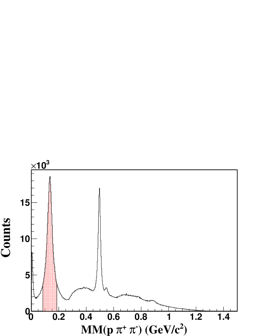

Figs. 3, 3 and 4 show the reconstructed , , and respectively. The fitted values of the mass and Gaussian width of the , and are shown in Table 1. The is selected, for final calculation, by taking a cut in addition to the above mentioned cuts. Here, and are the fitted values of mass and width of the . See Table 1.
| particle | mass (GeV/c | width, (GeV/c | cuts applied |
|---|---|---|---|
| 0.4990 | 0.0036 | collinearity cut | |
| 0.1351 | 0.0169 | collinearity cut and selected | |
| 1.1883 | 0.0056 | collinearity cut, and selected |
IV Background subtraction
One of the sources of physics background is from production. Because decays to , it is also present in the sidebands of the . There is also a background due to direct production of the final state particles. The dotted line in Fig. 4 shows the missing mass distribution of the two oppositely charged pions after selecting wide sidebands from both sides of the in the distribution. Here, we take for the left sideband and for the right sideband, where and are the fitted values of the mass and Gaussian width of the (see Table 1). No normalization or scaling was applied. As we can see from Fig. 4, the background is perfectly described by the sidebands of the . We also checked the sideband distributions for the different kinematic bins used in the final results, and we found that the sidebands perfectly describe the background in all kinematic bins. Therefore, we used the sidebands of the under the peak for the background subtraction. We checked the background due to misidentification of kaons as protons and it was negligible.
V Detector acceptance correction
The Monte Carlo (MC) events were generated uniformly in the () phase space with a uniform angular distribution of the proton in the rest frame, i.e. with zero polarization. The CLAS GEANT based simulation tool was used to simulate the passage of the generated events through CLAS. Then, the accepted events were reconstructed by using the CLAS reconstruction software. Distributions of different kinematic variables from the accepted MC events were compared with the experimental data and showed good agreement. The up and down acceptance distributions with respect to the production plane were equal to within less than 1%. See Sec. VI for the definition of the up and down distributions. The polarization calculated from the accepted events was less than in the entire kinematic range of our measurement. Therefore, the effects due to detector acceptance and false asymmetry are negligible. These MC events were used for the acceptance correction.
To check the quality of the acceptance correction, we also generated MC events with 100% polarization by using the same MC generator and reconstructed by the CLAS reconstruction software. We applied the acceptance correction to the accepted events by using the acceptance function obtained from unpolarized MC events as explained above. Then, we calculated the polarization of the acceptance corrected events and found that it is close to 100% within . See Section VI for a discussion of the polarization calculation method. From these studies we concluded that our acceptance correction method works well, and the overall systematic uncertainty on the observed polarization due to the detector acceptance and bias is 2%.
VI Analysis Method and Results
The is produced via the electromagnetic interaction, which conserves parity. However, it decays to a proton and via the parity violating weak interaction. Therefore, the polarization of the can be measured from the angular distribution of one of its decay products in the rest frame. Below we take the direction normal to the production plane as the -axis (transversity frame Beaupre:1973re ), the direction along the momentum vector as the -axis, and the -axis is chosen in order to make a right-handed coordinate system, as shown in Fig. 5. Corresponding unit-vectors are given by
| (4) | ||||
| (5) | ||||
| (6) |

The angular distribution of the proton in the rest frame is given by Cronin:1963zb
| (7) |
where is the angle between the proton momentum vector and the quantization axis of the along , is the transverse component of the polarization of the , is a measure of the degree of parity mixing Lee:1957qs and its value for the above decay channel is pdg . is the total number of events. The longitudinal component of the polarization vanishes. Eq. (7) can be split into up () and down () distributions with respect to the production plane:
| (8) | ||||
| (9) |
Using these two equations, one can write
| (10) |
Here, varies from 0 to 1 only. The benefit of using the ratio of the up and down distributions is essentially to cancel the effect of the acceptance correction, assuming that the acceptance corrections for the up and down distributions are the same. However, we didn’t rely on such an assumption and applied acceptance corrections. Eq. (10) can be integrated over to obtain
| (11) |
In Eq. (11), the distributions are corrected bin-by-bin in and the photon energy for the CLAS acceptance.


Fig. 6 shows the polarization with respect to the production angle of in the CM frame, , for different bins of photon energy from 1.0 GeV to 3.5 GeV. Fig. 7 shows the polarization with respect to the photon energy for different bins. The error bars on the points are statistical uncertainties, the bands on the horizontal axis are the systematic uncertainties. The data points corresponding to Figs. 6 and 7 are shown in Tables 2, 3 and 4.
VII Systematic Uncertainties
Systematic uncertainties are estimated from four different sources:
-
•
mass cut: we changed the width for the selection from to and the difference in polarizations obtained from these two selections is taken as a systematic uncertainty. The systematic uncertainty due to the mass cut varies up-to in most of the kinematic region.
-
•
collinearity cut: we changed the collinearity cut from to and the difference in polarizations obtained from these two cuts is taken as a systematic uncertainty. The systematic uncertainty due to the collinearity cut varies up-to in most of the kinematic region.
-
•
background subtraction: polarization calculated from the background events is taken as a systematic uncertainty. An explanation of the background events is given in Sec. IV. The systematic uncertainty due to the background subtraction varies up-to in most of the kinematic region.
-
•
acceptance correction: we did acceptance corrections to the data by using unpolarized MC events and 100% polarized MC events separately, and the difference in polarizations obtained from these two acceptance correction methods is taken as a systematic uncertainty. For the final polarization results, the unpolarized MC events were used for the acceptance corrections to the data, see Sec. V. The systematic uncertainty due to the acceptance correction varies up-to in most of the kinematic region.
The most significant contribution to the systematic uncertainty comes from the collinearity cut. The total systematic uncertainty for each bin is obtained by adding these four systematic uncertainties in that bin in quadrature and are shown by the grey bands on Figs. 6 and 7. Errors are also shown in the Tables 2, 3, and 4, along with the polarization values, where superscripts are statistical uncertainties and subscripts are systematic uncertainties.
| (GeV) / (GeV) | |||||||||||||||||||||
|---|---|---|---|---|---|---|---|---|---|---|---|---|---|---|---|---|---|---|---|---|---|
|
|
|
|
|
|
|
|||||||||||||||
| - | |||||||||||||||||||||
| - | |||||||||||||||||||||
| - | |||||||||||||||||||||
| - | |||||||||||||||||||||
| - | |||||||||||||||||||||
| - | |||||||||||||||||||||
| - | |||||||||||||||||||||
| - | |||||||||||||||||||||
| - | |||||||||||||||||||||
| (GeV) / (GeV) | |||||||||||||||||||||
|
|
|
|
|
|
|
|||||||||||||||
| - | |||||||||||||||||||||
| - | |||||||||||||||||||||
| - | |||||||||||||||||||||
| - | |||||||||||||||||||||
| - | - | - | |||||||||||||||||||
| - | - | - | |||||||||||||||||||
| - | - | - | |||||||||||||||||||
| - | - | - | |||||||||||||||||||
| - | - | - | - | - | - | ||||||||||||||||
| (GeV) | (GeV) | ||||||||
| - | - | - | - | - | - | - | - | ||
| - | - | ||||||||
| - | - | ||||||||
| - | - | ||||||||
| - | - | ||||||||
| - | - | ||||||||
| - | - | ||||||||
| - | - | ||||||||
| - | - | - | |||||||
| - | - | - | |||||||
| - | - | - | - | ||||||
VIII Discussion and Summary
We have measured the transverse polarization () in photoproduction on a hydrogen target in the photon beam energy range 1.0-3.5 GeV (which corresponds to 1.66-2.73 GeV). The is significantly polarized in most of the kinematic region and its magnitude goes up to 95%. Fig. 8 shows the comparison of our result with SAPHIR Lawall:2005np for the corresponding kinematic region. Our results are in good agreement with SAPHIR but with better precision.

SU(6) symmetry and the idea based on a polarization of the quark Heller:1990gc produced from the sea suggest . However, it has been shown in Ref. Dey:2010hh that this symmetry between the and is broken explicitly in mid and forward angles of the hyperon in the CM frame. Comparison plots of the polarization of the and the Dey:2010hh are shown in Fig. 9. For comparison with Ref. Dey:2010hh , we used . Also, the direction is taken as the quantization axis in Ref. Dey:2010hh . Therefore, we have scaled our result by (Fig. 9 only). Because of the low statistics in the forward direction, we compared here data points for backward going only. We can see that the trend of the polarizations with CM energies, , in both cases is similar except with systematic differences of about 1 at GeV. Also, as we can see from Fig. 6 that the trend of the polarizations near the resonance regime ( GeV) and above the resonance regime ( GeV) is different. This might indicate that the production mechanisms in these two regimes are different. Recently, several resonances have been shown to exist at around 2 GeV Anisovich:2011ye ; Anisovich:2012ct . This difference in polarization might be due to the resonance effects of the different contributing s-channel states in these two mass ranges.

Because of low statistics, especially at high energy, and for the forward and backward directions, it is difficult to track the variation of the polarization with different kinematic variables. For better understanding of the mechanism of polarization in the photoproduction process, and to understand the polarization mechanism at higher energy and at higher transverse momentum (), measurements at even higher energies with good statistics are necessary.
IX Acknowledgments
We would like to acknowledge the outstanding efforts of the staff of the Accelerator and the Physics Divisions at Jefferson Lab that made the experiment possible. This work was supported in part by the Italian Istituto Nazionale di Fisica Nucleare, the French Centre National de la Recherche Scientifique and Commissariat à l’Energie Atomique, the U.S. Department of Energy and National Science Foundation, the National Research Foundation of Korea, and the United Kingdom’s Science and Technology Facilities Council. The Southeastern Universities Research Association (SURA) operates the Thomas Jefferson National Accelerator Facility for the United States Department of Energy under contract DEAC05-84ER40150.
References
- (1) N. Isgur and G. Karl, Phys. Rev. D 18, 4187 (1978); Phys. Rev. D 19, 2653 (1979).
- (2) S. Capstick, Phys. Rev. D 46, 2864 (1992); S. Capstick and W. Roberts, Phys. Rev. D 49, 4570 (1994); S. Capstick and W. Roberts, Phys. Rev. D 57, 4301 (1998).
- (3) R. Schumacher, Eur. Phys. J. A 35, 299 (2008).
- (4) J. W. C. McNabb et al. [The CLAS Collaboration], Phys. Rev. C69, 042201 (2004).
- (5) A. Lleres et al., Eur. Phys. J. A31, 79-93 (2007).
- (6) K. H. Glander et al., Eur. Phys. J. A19, 251-273 (2004).
- (7) R. Bradford et al. [CLAS Collaboration], Phys. Rev. C 73, 035202 (2006)
- (8) R. K. Bradford et al. [CLAS Collaboration], Phys. Rev. C 75, 035205 (2007)
- (9) M. E. McCracken et al. [CLAS Collaboration], Phys. Rev. C 81, 025201 (2010)
- (10) B. Dey et al. [CLAS Collaboration], Phys. Rev. C82, 025202 (2010).
- (11) A. V. Anisovich et al., Eur. Phys. J. A 47, 153 (2011)
- (12) A. V. Anisovich et al., Eur. Phys. J. A 48, 88 (2012)
- (13) D. S. Carman et al. [CLAS Collaboration], Phys. Rev. Lett. 90, 131804 (2003)
- (14) D. S. Carman et al. [CLAS Collaboration], Phys. Rev. C 79, 065205 (2009)
- (15) J. J. Sakurai, Invariance Principles and Elementary Particles, Princeton University Press, Princeton, New Jersey, USA (1964).
- (16) K. J. Heller, J. Phys. Colloq. 51, 163 (1990).
- (17) R. Lawall et al., Eur. Phys. J. A 24, 275 (2005).
- (18) B. A. Mecking et al., Nucl. Instrum. Meth. A 503, 513 (2003).
- (19) D. I. Sober et al., Nucl. Instrum. Meth. A 440, 263 (2000).
- (20) M. Gell-Mann and A. Pais, Phys. Rev. 97, 1387 (1955).
- (21) A. Pais and O. Piccioni, Phys. Rev. 100, 1487 (1955).
- (22) J. Beringer et al. (Particle Data Group), Phys. Rev. D86, 010001 (2012).
- (23) E. Pasyuk [CLAS Collaboration], Energy loss corrections for charged particles in CLAS, CLAS-NOTE:2007-016.
- (24) J. V. Beaupre et al. [Aachen-Berlin-CERN-Cracow-London-Vienna-Warsaw Collaboration], Nucl. Phys. B 49, 405 (1972).
- (25) J. W. Cronin and O. E. Overseth, Phys. Rev. 129, 1795 (1963).
- (26) T. D. Lee and C. N. Yang, Phys. Rev. 108, 1645 (1957).