Casimir interaction energies for magneto-electric $\delta$-function plates.

Abstract

We present boundary conditions for the electromagnetic fields on a $\delta$-function plate, having both electric and magnetic properties, sandwiched between two magneto-electric semi-infinite half spaces. The optical properties for an isolated $\delta$-function plate are shown to be independent of the longitudinal material properties of the plate. The Casimir-Polder energy between an isotropically polarizable atom and a magneto-electric $\delta$-function plate is attractive for a purely electric $\delta$-function plate, repulsive for a purely magnetic $\delta$-function plate, and vanishes for the simultaneous perfect conductor limit of both electric and magnetic properties of the $\delta$-function plate. The interaction energy between two identical $\delta$-function plates is always attractive. It can be attractive or repulsive when the plates have electric and magnetic properties interchanged and reproduces Boyer’s result for the interaction energy between perfectly conducting electric and magnetic plates. The change in the Casimir-Polder energy in the presence of a $\delta$-function plate on a magneto-electric substrate is substantial when the substrate is a weak dielectric.

1 Introduction

Infinitesimally thin perfectly conducting surfaces have often been used at least since the first rigorous exact solution of diffraction of a plane wave by a half-plate of infinitesimal thickness given by Sommerfeld in 1896 [1, 2]. Another iconic example, in the field of Casimir physics, is Boyer’s calculation of the repulsive Casimir pressure for such an infinitesimally thin perfectly conducting spherical shell [3]. A closed perfectly conducting infinitesimally thin surface is like an “electric wall” that decouples two regions of space [4]. Therefore, it is sufficient to consider only the region of interest where the interaction is occurring. However, examples like an infinitesimally thin half plane or a perfectly conducting plate with an aperture [5] require the consideration of the other side of the perfectly conducting surface.

Boundary conditions on an electric material of infinitesimal thickness were first derived by Barton in Refs. [6, 7, 8] who observed that an infinitesimally thin conducting surface imposes non-trivial boundary conditions on the electromagnetic fields and in Refs. [9, 10] considered “a fluid model of an infinitesimally thin plasma sheet”. These boundary conditions were generalized for magneto-electric materials in Ref. [11].

References [12, 13] were the first to use a $\delta$-function potential to mathematically represent an infinitesimally thin surface. Robaschik and Wieczorek in [14] proposed that two different boundary conditions could be satisfied on a perfectly conducting electric $\delta$-function plate, and Bordag in [15] further claimed that the interaction energy between an atom and a $\delta$-function plate satisfying these two boundary conditions are not identical. These confusions were discussed in detail and resolved in [11] in which we showed that the electric Green’s dyadic obtained using both boundary conditions were identical and therefore corresponded to the same physical situation.

In [11] we derived the boundary conditions on a $\delta$-function plate having both electric and magnetic properties, which will be termed as a magneto-electric $\delta$-function plate in this paper, and showed that such a plate can be realized physically in the so-called “thin-plate” limit. We presented results for the interaction energy between two such $\delta$-function plates and between an atom and a $\delta$-function plate when they have purely electric properties.

In this paper we study examples involving magneto-electric $\delta$-function plates. In the following section, we briefly present the derivation of the boundary conditions on an infinitesimally thin magneto-electric $\delta$-function plate sandwiched between two magneto-electric semi-infinite half spaces and present solutions for the magnetic and electric Green’s functions. In the thin-plate limit, $\zeta d\ll\sqrt{\zeta_{p}d}\ll 1$, where $\omega_{p}^{2}=\zeta_{p}/d$ is the plasma frequency of the material, a vanishing thickness $d$ of the plate reproduces the optical properties of an electric $\delta$-function plate. The suggestion is that a theoretical calculation, for example, for a corrugated surface, could be greatly simplified if the boundaries in consideration could be approximated by their respective $\delta$-function forms.

In the subsequent sections we consider the change in the Casimir-Polder energy due to the presence of a magneto-electric $\delta$-function plate on the surface of a magneto-electric semi-infinite half space and the Casimir interaction energy between two magneto-electric $\delta$-function plates. In experiments thin films of metals are grown on a substrate and their properties are not continuous, transitioning from insulator to metal abruptly. This is in contrast to the $\delta$-function plate, which has continuous properties, and it is therefore not clear how to compare our results with experimentally realizable thin metal films. On the other hand, it is well known that a coat of a thin dielectric film on a metal surface changes the reflectivity of the metal surface. Thus in principle, one could think of varying the Casimir interaction energy between two surfaces by coating them with the physically realizable $\delta$-function plates discussed in Sec. 3.

2 Boundary conditions on an infinitesimally thin magneto-electric $\delta$-function plate

We consider a magneto-electric $\delta$-function plate sandwiched between two uniaxial magneto-electric materials as shown in Fig. 1.

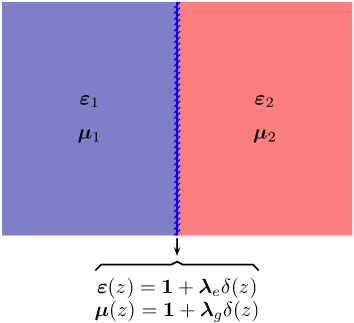
Figure 1: A magneto-electric $\delta$-function plate sandwiched between two magneto-electric semi-infinite slabs.

The electric permittivity $\varepsilon$ and the magnetic permeability $\mu$ for this system are described by

$$\bm{\varepsilon}(z)=\varepsilon^{\perp}(z)\,{\bf 1}_{\perp}+\varepsilon^{||}(z)\,\hat{\bf z}\,\hat{\bf z}\qquad\text{and}\qquad\bm{\mu}(z)=\mu^{\perp}(z)\,{\bf 1}_{\perp}+\mu^{||}(z)\,\hat{\bf z}\,\hat{\bf z},$$ (1)

where $z=a$ is the position of the interface, and

$$\varepsilon^{\perp,||}(z) = 1+(\varepsilon^{\perp,||}_{1}-1)\theta(a-z)+(\varepsilon^{\perp,||}_{2}-1)\theta(z-a)+\lambda^{\perp,||}_{e}\delta(z-a),$$ (2a)

$$\mu^{\perp,||}(z) = 1+(\mu^{\perp,||}_{1}-1)\theta(a-z)+(\mu^{\perp,||}_{2}-1)\theta(z-a)+\lambda^{\perp,||}_{g}\delta(z-a).$$ (2b)

The electric permittivity and magnetic permeability are in general frequency dependent. The Maxwell equations in the absence of charges and currents, in frequency space, are

$${\bm{\nabla}}\times{\bf E}=i\omega{\bf B}\qquad\text{and}\qquad-{\bm{\nabla}}\times{\bf H}=i\omega({\bf D}+{\bf P}),$$ (3)

where we assume the fields ${\bf D}$ and ${\bf B}$ are linearly dependent on the electric and magnetic fields ${\bf E}$ and ${\bf H}$ as

$${\bf D}({\bf x},\omega)={\bm{\varepsilon}}({\bf x};\omega)\cdot{\bf E}({\bf x},\omega)\qquad\text{and}\qquad{\bf B}({\bf x},\omega)={\bm{\mu}}({\bf x};\omega)\cdot{\bf H}({\bf x},\omega),$$ (4)

and ${\bf P}$ is an external source of polarization.

2.1 Boundary conditions

The Maxwell equations in Eq. (3) decouple into transverse electric (TE) and transverse magnetic (TM) modes for planar geometries. The boundary conditions on the electric and magnetic fields ${\bf E}$ and ${\bf H}$ are obtained by integrating across the $\delta$-function boundary. We get additional contributions to the standard boundary conditions at the interface of two media due to the presence of the magneto-electric $\delta$-function plate as follows:

TM TE

$$E_{1}\Big{|}^{z=a+}_{z=a-} =i\omega\lambda_{g}^{\perp}H_{2}(a), H_{1}\Big{|}^{z=a+}_{z=a-} =-i\omega\lambda_{e}^{\perp}E_{2}(a),$$ (5a)

$$H_{2}\Big{|}^{z=a+}_{z=a-} =i\omega\lambda_{e}^{\perp}E_{1}(a), E_{2}\Big{|}^{z=a+}_{z=a-} =-i\omega\lambda_{g}^{\perp}H_{1}(a),$$ (5b)

$$D_{3}\Big{|}^{z=a+}_{z=a-} =-ik_{\perp}\lambda_{e}^{\perp}E_{1}(a), B_{3}\Big{|}^{z=a+}_{z=a-} =-ik_{\perp}\lambda_{g}^{\perp}H_{1}(a).$$ (5c)

In addition we get the constraints,

$$\lambda_{e}^{||}E_{3}(a)=0\qquad\text{and}\qquad\lambda_{g}^{||}H_{3}(a)=0,$$ (6)

which imply that optical properties of the magneto-electric $\delta$-function plate are necessarily anisotropic unless $E_{3}(a)=0$ and $H_{3}(a)=0$. These restrictions are implicit in the model considered by Barton [9].

2.2 Green’s functions

We use the Green’s function technique to obtain the electric and magnetic fields ${\bf E}$ and ${\bf H}$:

$${\bf E}({\bf x})=\int d^{3}x^{\prime}\,{\bm{\Gamma}}({\bf x},{\bf x}^{\prime})\cdot{\bf P}({\bf x}^{\prime})\qquad\text{and}\qquad{\bf H}({\bf x})=\int d^{3}x^{\prime}\,{\bm{\Phi}}({\bf x},{\bf x}^{\prime})\cdot{\bf P}({\bf x}^{\prime}),$$ (7)

in terms of the electric Green’s dyadic ${\bm{\Gamma}}({\bf x},{\bf x}^{\prime})$ and magnetic Green’s dyadic ${\bm{\Phi}}({\bf x},{\bf x}^{\prime})$ respectively. Using translational symmetry we can Fourier transform the Green’s dyadics in the $xy$-plane, for example,

$${\bm{\Gamma}}({\bf x},{\bf x}^{\prime};\omega)=\int\frac{d^{2}k_{\perp}}{(2\pi)^{2}}\,e^{i{\bf k}_{\perp}\cdot({\bf x}-{\bf x}^{\prime})_{\perp}}{\bm{\gamma}}(z,z^{\prime};{\bf k}_{\perp},\omega).$$ (8)

The reduced Green’s dyadics ${\bm{\gamma}}(z,z^{\prime})$ and ${\bm{\phi}}(z,z^{\prime})$, in the coordinate system where ${\bm{k}}_{\perp}$ lies in x direction, are

$${\bm{\gamma}}=\left[\begin{array}[]{ccc}\frac{1}{\varepsilon^{\perp}}\frac{\partial}{\partial z}\frac{1}{\varepsilon^{\prime\perp}}\frac{\partial}{\partial z^{\prime}}g^{H}&0&\frac{1}{\varepsilon^{\perp}}\frac{\partial}{\partial z}\frac{ik_{\perp}}{\varepsilon^{\prime||}}g^{H}\\[5.69054pt] 0&\omega^{2}g^{E}&0\\[5.69054pt] -\frac{ik_{\perp}}{\varepsilon^{||}}\frac{1}{\varepsilon^{\prime\perp}}\frac{\partial}{\partial z^{\prime}}g^{H}&0&-\frac{ik_{\perp}}{\varepsilon^{||}}\frac{ik_{\perp}}{\varepsilon^{\prime||}}g^{H}\end{array}\right]$$ (9)

and

$${\bm{\phi}}=i\omega\left[\begin{array}[]{ccc}0&\frac{1}{\mu^{\perp}}\frac{\partial}{\partial z}g^{E}&0\\[5.69054pt] \frac{1}{\varepsilon^{\prime\perp}}\frac{\partial}{\partial z^{\prime}}g^{H}&0&\frac{ik_{\perp}}{\varepsilon^{\prime||}}g^{H}\\[5.69054pt] 0&-\frac{ik_{\perp}}{\mu^{||}}g^{E}&0\end{array}\right],$$ (10)

where we have suppressed the $z$ and $z^{\prime}$ dependence and $\varepsilon^{\prime}$ is evaluated at point $z^{\prime}$. In Eq. (9) we have omitted a contact term involving $\delta(z-z^{\prime})$, which does not contribute to interaction energies between disjoint objects. The magnetic Green’s function $g^{H}(z,z^{\prime})$ and the electric Green’s function $g^{E}(z,z^{\prime})$ satisfy

$$\left[-\frac{\partial}{\partial z}\frac{1}{\varepsilon^{\perp}(z)}\frac{\partial}{\partial z}+\frac{k_{\perp}^{2}}{\varepsilon^{||}(z)}-\omega^{2}\mu^{\perp}(z)\right]g^{H}(z,z^{\prime}) = \delta(z-z^{\prime}),$$ (11a)

$$\left[-\frac{\partial}{\partial z}\frac{1}{\mu^{\perp}(z)}\frac{\partial}{\partial z}+\frac{k_{\perp}^{2}}{\mu^{||}(z)}-\omega^{2}\varepsilon^{\perp}(z)\right]g^{E}(z,z^{\prime}) = \delta(z-z^{\prime}),$$ (11b)

where the material properties $\varepsilon^{\perp}(z)$ and $\mu^{\perp}(z)$ are given by Eqs. (2). We obtain the boundary conditions on the magnetic Green’s functions using Eq. (5c) for TM mode,

$$g^{H}\Big{|}^{z=a+}_{z=a-} = \lambda^{\perp}_{e}\frac{1}{\varepsilon^{\perp}}\partial_{z}g^{H}\bigg{|}_{z=a},$$ (12a)

$$\frac{1}{\varepsilon^{\perp}}\partial_{z}g^{H}\bigg{|}^{z=a+}_{z=a-} = \zeta^{2}\lambda^{\perp}_{g}g^{H}\Big{|}_{z=a}.$$ (12b)

Similarly, using Eq. (5c) for TE mode, the boundary conditions on the electric Green’s function are

$$g^{E}\Big{|}^{z=a+}_{z=a-} = \lambda^{\perp}_{g}\frac{1}{\mu^{\perp}}\partial_{z}g^{E}\bigg{|}_{z=a},$$ (13a)

$$\frac{1}{\mu^{\perp}}\partial_{z}g^{E}\bigg{|}^{z=a+}_{z=a-} = \zeta^{2}\lambda^{\perp}_{e}g^{E}\Big{|}_{z=a}.$$ (13b)

Here $\zeta$ is the imaginary frequency obtained after a Euclidean rotation. We evaluate quantities that are discontinuous on the magneto-electric $\delta$-function plate using the averaging prescription described in [16].

The solution for the magnetic Green’s function satisfying the boundary conditions in Eq. (12) is

$$g^{H}(z,z^{\prime})=\begin{cases}\frac{1}{2\bar{\kappa}^{H}_{1}}\Big{[}e^{-\kappa^{H}_{1}|z-z^{\prime}|}+r^{H}_{12}\,e^{-\kappa^{H}_{1}|z-a|}e^{-\kappa^{H}_{1}|z^{\prime}-a|}\Big{]},&\text{if}\quad z,z^{\prime}<a,\\[5.69054pt] \frac{1}{2\bar{\kappa}^{H}_{2}}\Big{[}e^{-\kappa^{H}_{2}|z-z^{\prime}|}+r^{H}_{21}\,e^{-\kappa^{H}_{2}|z-a|}e^{-\kappa^{H}_{2}|z^{\prime}-a|}\Big{]},&\text{if}\quad a<z,z^{\prime},\\[5.69054pt] \frac{1}{2\bar{\kappa}^{H}_{2}}\,t^{H}_{21}\,e^{-\kappa^{H}_{1}|z-a|}e^{-\kappa^{H}_{2}|z^{\prime}-a|},&\text{if}\quad z<a<z^{\prime},\\[5.69054pt] \frac{1}{2\bar{\kappa}^{H}_{1}}\,t^{H}_{12}\,e^{-\kappa^{H}_{2}|z-a|}e^{-\kappa^{H}_{1}|z^{\prime}-a|},&\text{if}\quad z^{\prime}<a<z,\end{cases}$$ (14)

where the reflection and transmission coefficients are

$$r^{H}_{ij}=\frac{\bar{\kappa}^{H}_{i}\Big{(}1+\frac{\lambda^{\perp}_{e}\bar{\kappa}^{H}_{j}}{2}\Big{)}\Big{(}1-\frac{\lambda^{\perp}_{g}\zeta^{2}}{2\bar{\kappa}^{H}_{i}}\Big{)}-\bar{\kappa}^{H}_{j}\Big{(}1-\frac{\lambda^{\perp}_{e}\bar{\kappa}^{H}_{i}}{2}\Big{)}\Big{(}1+\frac{\lambda^{\perp}_{g}\zeta^{2}}{2\bar{\kappa}^{H}_{j}}\Big{)}}{\bar{\kappa}^{H}_{i}\Big{(}1+\frac{\lambda^{\perp}_{e}\bar{\kappa}^{H}_{j}}{2}\Big{)}\Big{(}1+\frac{\lambda^{\perp}_{g}\zeta^{2}}{2\bar{\kappa}^{H}_{i}}\Big{)}+\bar{\kappa}^{H}_{j}\Big{(}1+\frac{\lambda^{\perp}_{e}\bar{\kappa}^{H}_{i}}{2}\Big{)}\Big{(}1+\frac{\lambda^{\perp}_{g}\zeta^{2}}{2\bar{\kappa}^{H}_{j}}\Big{)}},$$ (15a)

$$t^{H}_{ij}=\frac{\bar{\kappa}^{H}_{i}\Big{(}1+\frac{\lambda^{\perp}_{e}\bar{\kappa}^{H}_{i}}{2}\Big{)}\Big{(}1-\frac{\lambda^{\perp}_{g}\zeta^{2}}{2\bar{\kappa}^{H}_{i}}\Big{)}+\bar{\kappa}^{H}_{i}\Big{(}1-\frac{\lambda^{\perp}_{e}\bar{\kappa}^{H}_{i}}{2}\Big{)}\Big{(}1+\frac{\lambda^{\perp}_{g}\zeta^{2}}{2\bar{\kappa}^{H}_{i}}\Big{)}}{\bar{\kappa}^{H}_{i}\Big{(}1+\frac{\lambda^{\perp}_{e}\bar{\kappa}^{H}_{j}}{2}\Big{)}\Big{(}1+\frac{\lambda^{\perp}_{g}\zeta^{2}}{2\bar{\kappa}^{H}_{i}}\Big{)}+\bar{\kappa}^{H}_{j}\Big{(}1+\frac{\lambda^{\perp}_{e}\bar{\kappa}^{H}_{i}}{2}\Big{)}\Big{(}1+\frac{\lambda^{\perp}_{g}\zeta^{2}}{2\bar{\kappa}^{H}_{j}}\Big{)}},$$ (15b)

with

$$\kappa_{i}^{H}=\sqrt{k_{\perp}^{2}\frac{\varepsilon^{\perp}_{i}}{\varepsilon^{||}_{i}}+\zeta^{2}\varepsilon^{\perp}_{i}\mu^{\perp}_{i}}\qquad\text{and}\qquad\bar{\kappa}^{H}_{i}=\frac{\kappa^{H}_{i}}{\varepsilon^{\perp}_{i}}=\sqrt{\frac{k_{\perp}^{2}}{\varepsilon^{\perp}_{i}\varepsilon^{||}_{i}}+\zeta^{2}\frac{\mu^{\perp}_{i}}{\varepsilon^{\perp}_{i}}}.$$ (16)

The electric Green’s function is obtained by replacing ${\bm{\varepsilon}}\leftrightarrow{\bm{\mu}}$ and $H\to E$ everywhere. Notice that the reflection and transmission coefficients are independent of $\lambda^{||}_{e}$ and $\lambda^{||}_{g}$, which implies that the optical properties of the magneto-electric $\delta$-function plates are independent of the longitudinal components of the material properties.

2.3 Green’s function for an isolated magneto-electric $\delta$-function plate in vacuum

Green’s function for a magneto-electric $\delta$-function plate in vacuum is obtained by setting $\varepsilon^{\perp}_{i}=\varepsilon^{||}_{i}=1$ and $\mu^{\perp}_{i}=\mu^{||}_{i}=1$ in Eq. (15). The magnetic Green’s function in compact form is

$$g^{H}(z,z^{\prime})=\frac{1}{2\kappa}e^{-\kappa|z-z^{\prime}|}+\big{[}r^{H}_{g}+\text{sgn}(z-a)\text{sgn}(z^{\prime}-a)\,r^{H}_{e}\big{]}\frac{1}{2\kappa}e^{-\kappa|z-a|}e^{-\kappa|z^{\prime}-a|},$$ (17)

where $\kappa^{2}=k_{\perp}^{2}+\zeta^{2}$. The electric and magnetic reflection coefficients are

$$r^{H}_{e}=\frac{\lambda^{\perp}_{e}}{\lambda^{\perp}_{e}+\frac{2}{\kappa}},\qquad\text{and}\qquad r^{H}_{g}=-\frac{\lambda^{\perp}_{g}}{\lambda^{\perp}_{g}+\frac{2\kappa}{\zeta^{2}}},$$ (18)

which are defined for the cases $\lambda_{g}^{\perp}$ and $\lambda_{e}^{\perp}$ being zero, respectively. The total reflection coefficient for the magnetic mode is $r^{H}=r^{H}_{g}+r^{H}_{e}$. The TE reflection coefficient $r^{E}$ is obtained by replacing $e\leftrightarrow g$ and $H\to E$ in Eq. (18). The TM and TE reflection coefficients vanish when simultaneously $\lambda_{e}\to\infty$ and $\lambda_{g}\to\infty$: The plate behaves like a perfect electric and perfect magnetic conductor, which we will refer as perfect magneto-electric conductor. This implies that a perfectly conducting magneto-electric $\delta$-function plate becomes transparent to the electromagnetic fields.

3 Physical realization of an electric $\delta$-function plate: Thin plate limit

The $\delta$-function potential used to describe a magneto-electric plate in Sec. 2 is a mathematical tool, which gives calculational ease. In case of a perfect conductor a $\delta$-function potential still serves as an accurate description of the physical system because the perfect conductor decouples the two regions in space. However, to describe a thin dielectric material slab of thickness $d$ using a $\delta$-function potential we need to use approximations on the material properties in the limit $d\to 0$. We can write a $\delta$-function as difference of two step functions describing a slab of thickness $d$ and take the limit $d\to 0$ after dividing out the thickness. Multiplying this construction by ${\bm{\lambda}_{e}}$, we can read off the susceptibility of the slab as ${\bm{\lambda}_{e}}/d$.

The transverse magnetic and transverse electric reflection coefficient of a material slab of thickness $d$ is

$$r_{\text{thick}}^{H}=-\frac{\left(\frac{\bar{\kappa}^{H}-\kappa}{\bar{\kappa}^{H}+\kappa}\right)(1-e^{-2\kappa^{H}d})}{\left[1-\left(\frac{\bar{\kappa}^{H}-\kappa}{\bar{\kappa}^{H}+\kappa}\right)^{2}e^{-2\kappa^{H}d}\right]}\qquad\text{and}\qquad r_{\text{thick}}^{E}=-\frac{\left(\frac{\kappa^{E}-\kappa}{\kappa^{E}+\kappa}\right)(1-e^{-2\kappa^{E}d})}{\left[1-\left(\frac{\kappa_{i}^{E}-\kappa}{\kappa^{E}+\kappa}\right)^{2}e^{-2\kappa^{E}d}\right]}.$$ (19)

Naively taking the $d\to 0$ limit yields vanishing reflection coefficients. However, in the thin-plate limit,

$$\zeta^{2}\ll\frac{\zeta_{p}}{d}\ll\frac{1}{d^{2}},\qquad\text{and}\qquad k_{\perp}^{2}\ll\frac{\zeta_{p}}{d}\ll\frac{1}{d^{2}},$$ (20)

where $\zeta_{p}=\omega_{p}^{2}d$ is the characteristic wave number of the material, the reflection coefficients for TM- and TE-modes exactly reproduce the reflection coefficients for a purely electric $\delta$-function plate:

$$r_{\text{thick}}^{H}\xrightarrow[k_{\perp}d\ll\sqrt{\zeta_{p}d}\ll 1]{\zeta d\ll\sqrt{\zeta_{p}d}\ll 1}r_{e}^{H}=\frac{\lambda_{e}^{\perp}}{\lambda_{e}^{\perp}+\frac{2}{\kappa}},\quad\text{and}\quad r_{\text{thick}}^{E}\xrightarrow[k_{\perp}d\ll\sqrt{\zeta_{p}d}\ll 1]{\zeta d\ll\sqrt{\zeta_{p}d}\ll 1}r_{e}^{E}=-\frac{\lambda_{e}^{\perp}}{\lambda_{e}^{\perp}+\frac{2\kappa}{\zeta^{2}}}.$$ (21)

It is worth noting that the reflection coefficients for both a thick slab and a $\delta$-function plate give same value in the perfect conductor limit, i.e., when the electrical permittivity goes to infinity.

4 Interaction energy between an electrically polarizable atom and a magneto-electric $\delta$-function plate

In this section we consider the interaction of an atom with anisotropic electric polarizability ${\bm{\alpha}}=\text{diag}(\alpha^{\perp},\alpha^{\perp},\alpha^{||})$ with a magneto-electric $\delta$-function plate.

4.1 Atom interacting with a magneto-electric $\delta$-function plate in vacuum

For the first case let us assume that the magneto-electric $\delta$-function plate is a stand-alone plate interacting with an electrically polarizable atom separated by a distance $a$, as shown in Fig. 2(a).

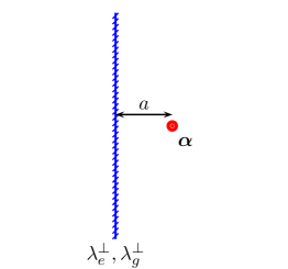
(a) Magneto-electric $\delta$-function plate

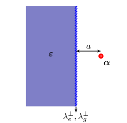
(b) Magneto-electric $\delta$-function plate on a dielectric slab

Figure 2: Anisotropic atom in front of 2(a) a magneto-electric $\delta$-function plate, versus 2(b) a magneto-electric $\delta$-function plate on an anisotropic dielectric slab.

The Casimir-Polder energy between an anisotropic atom and a magneto-electric $\delta$-function plate for this case evaluates to

$$E_{\delta\text{-atom}}=-2\pi\int_{-\infty}^{\infty}\frac{d\zeta}{2\pi}\int\frac{d^{2}k_{\perp}}{(2\pi)^{2}}\,\frac{e^{-2\kappa a}}{2\kappa}\Big{[}\alpha^{\perp}(\kappa^{2}r^{H}-\zeta^{2}r^{E})+\alpha^{||}k_{\perp}^{2}\,r^{H}\Big{]},$$ (22)

where the TM and TE reflection coefficients for a $\delta$-function plate are provided in Sec. 2.3. More specifically, the TM reflection coefficient

$$r^{H}=\frac{\lambda^{\perp}_{e}}{\lambda^{\perp}_{e}+\frac{2}{\kappa}}-\frac{\lambda^{\perp}_{g}}{\lambda^{\perp}_{g}+\frac{2\kappa}{\zeta^{2}}}$$ (23)

and TE reflection coefficient $r^{E}$ is obtained by replacing $e\leftrightarrow g$ and $H\to E$ in Eq. (23). In the retarded limit we replace atomic polarizabilities by their static limits.

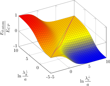
Figure 3: The variation of the Casimir-Polder interaction energy between an isotropic atom and a magneto-electric $\delta$-function plate in units of the magnitude of the usual Casimir-Polder interaction energy between an isotropic atom and a perfect electrically conducting plate as a function of $\ln\frac{\lambda^{\perp}_{e}}{a}$ and $\ln\frac{\lambda^{\perp}_{g}}{a}$.

In Fig. 3 we show the variation of the Casimir-Polder energy given in Eq. (22) with respect to the electric and magnetic properties of the magneto-electric $\delta$-function plate in units of the distance $a$ between the plates. We set $\alpha^{\perp}=\alpha^{||}$. The energy is normalized relative to the magnitude of the usual Casimir-Polder energy for an isotropic atom interacting with a perfect electric conductor. It is of interest to note that the interaction energy is always negative when the plate is purely electric and always positive when the plate is purely magnetic. The transition from a negative to a positive value of the energy occurs along a curve in the $\lambda^{\perp}_{e}$-$\lambda^{\perp}_{g}$ parameter space. In particular, the interaction energy vanishes for

$$\frac{\lambda^{\perp}_{e}}{a} = \frac{3}{7}\frac{\lambda^{\perp}_{g}}{a}\qquad\qquad\qquad\text{for the weak coupling limit}\left(\lambda^{\perp}_{e,g}\ll a\right),$$ (24a)

$$\frac{\lambda^{\perp}_{e}}{a} = \frac{256}{45}\frac{1}{\pi^{3/2}}\sqrt{\frac{\lambda^{\perp}_{g}}{a}}\qquad\text{for the strong coupling limit}\left(\lambda^{\perp}_{e,g}\gg a\right),$$ (24b)

to the leading order. Interestingly for the strong coupling case the interaction energy scales differently for the magnetic coupling $\lambda^{\perp}_{g}$ as compared to the electric coupling $\lambda^{\perp}_{e}$. Furthermore, the force between an isotropic atom and a magneto-electric $\delta$-function plate changes sign for different combination of $\lambda^{\perp}_{e}$ and $\lambda^{\perp}_{g}$. For example, for strong coupling the force vanishes for a condition of the form Eq. (24b) where numerical coefficient is replaced by $1536/315$.

The total reflection coefficients, $r^{H}$ and $r^{E}$, vanish for the special case when the plate behaves like a perfect magneto-electric conductor, i.e., $\lambda^{\perp}_{e}\to\infty$ and $\lambda^{\perp}_{g}\to\infty$. Thus, the Casimir-Polder interaction energy also vanishes for such a plate. This is a generic behavior for a perfectly conducting magneto-electric $\delta$-function plate. For a perfect electric conductor the TM and TE reflection coefficients are $r^{H}=1$ and $r^{E}=-1$ in which case we obtain the usual Casimir-Polder energy between an atom and a perfect electric conductor. In contrast, for a perfect magnetic conductor $r^{H}=-1$ and $r^{E}=1$ we obtain a repulsive interaction energy of the same magnitude, as evident from Fig. 3.

4.2 Atom interacting with a magneto-electric $\delta$-function plate on a dielectric substrate

As a second example let us consider an anisotropic atom interacting with a magneto-electric $\delta$-function plate on a semi-infinite dielectric substrate as shown in Fig. 2(b). The Casimir-Polder energy is still expressed by Eq. (22) with the reflection coefficients, $r^{H}$ and $r^{E}$, now obtained from Eq. (15). We choose the semi-infinite material to be isotropic and non-magnetic to reduce the numbers of parameters in the analysis. Again we set $\alpha^{\perp}=\alpha^{||}$ for the atom. Figures 4(a) and 4(b) show the fractional change in the Casimir-Polder energy in the presence of a magneto-electric $\delta$-function plate compared to the absence of the magneto-electric $\delta$-function plate on the substrate. When the electric permittivity of the substrate material is low then the presence of the magneto-electric $\delta$-function plate increases the magnitude of the interaction energy depending on the material properties of the plate, while the variation is less strong in the case when the dielectric permittivity of the substrate material is high. The biggest effect occurs when $\lambda_{g}$ is large and $\lambda_{e}$ is small. In other words, the material with stronger properties dominates in the contribution to the interaction energy.

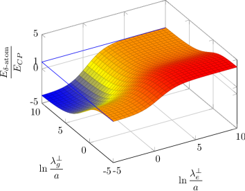
(a) Small electric permittivity

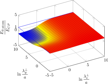
(b) High electric permittivity

Figure 4: Fractional change in the Casimir-Polder energy between an isotropic atom and a dielectric substrate of a fixed electric permittivity in the presence of the magneto-electric $\delta$-function plate relative to the Casimir-Polder energy in the absence of the plate as a function of the magnetic and electric properties of the plate, $\ln\frac{\lambda^{\perp}_{e}}{a}$ and $\ln\frac{\lambda^{\perp}_{g}}{a}$, respectively. The electric permittivity of the substrate material is 4(a) $\varepsilon=2$ and 4(b) $\varepsilon=100$.

5 Interaction energy between two magneto-electric $\delta$-function plates

In this section we evaluate the Casimir interaction energy between two magneto-electric $\delta$-function plates and study its variation as a function of the electric and magnetic properties of the plates. Let us consider two $\delta$-function plates described by the electric and magnetic properties, $\lambda^{\perp}_{ei}$ and $\lambda^{\perp}_{gi}$, respectively, with subscript $i=1,2$ representing the individual plates. The separation distance between the plates is $a$. See Fig. 5.

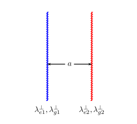
Figure 5: Parallel magneto-electric $\delta$-function plates separated by a distance $a$.

Considering that the TM and TE modes decouple for the planar geometry, the Casimir energy is conveniently expressed as

$$\frac{E_{\text{$\delta$-plate}}}{A}=\frac{1}{2}\int_{-\infty}^{\infty}\frac{d\zeta}{2\pi}\int\frac{d^{2}k_{\perp}}{(2\pi)^{2}}\Bigg{\{}\ln\Big{[}1-r_{1}^{H}r_{2}^{H}\,e^{-2\kappa a}\Big{]}+\ln\Big{[}1-r_{1}^{E}r_{2}^{E}\,e^{-2\kappa a}\Big{]}\Bigg{\}},$$ (25)

where the TM reflection coefficient for a single magneto-electric $\delta$-function plate is given in Eq. (23). The TE reflection coefficient $r^{E}$ is obtained by replacing $e\leftrightarrow g$ and $H\to E$. As mentioned before, the interaction energy vanishes when both plates are perfect magneto-electric conductors, as if plates are invisible to each other.

In Fig. 6(a) we plot the ratio of the Casimir interaction energy given in Eq. (25) to the magnitude of the Casimir energy between two perfectly conducting electric plates as a function of the electric and magnetic properties. For simplicity we have set $\lambda^{\perp}_{(e,g)1}=\lambda^{\perp}_{(e,g)2}$. The fractional change in the energy vanishes when there are no plates and when both the plates are simultaneously perfect electric and perfect magnetic conductors. In the case when both plates are either perfect electric conductors or perfect magnetic conductors, the energy ratio approaches $-1$ as expected. The ratio of the energies is always negative except when it goes to zero for two extreme cases described above. In addition, it is easy to check that the force between two identical magneto-electric $\delta$-function plates is always attractive by taking a negative derivative of Eq. (25) with respect to the separation distance $a$. Kenneth and Klich in [17] proved that for non-magnetic bodies “the Casimir force between two bodies related by reflection is always attractive, independent of the exact form of the bodies or dielectric properties”. The above example is a generalization of their theorem to magneto-electric bodies. The magnitude of the interaction energy, in general, is less than the usual Casimir energy between two perfect electrically conducting plates. The green line on the energy surface in Fig. 6(a) shows the value of the ratio of the interaction energies in the case $\lambda^{\perp}_{e}=\lambda^{\perp}_{g}$.

We plot another interesting case in Fig. 6(b), where we have considered the material properties of the two plates to be dual of each other, i.e. $\lambda^{\perp}_{e1}=\lambda^{\perp}_{g2}$ and $\lambda^{\perp}_{g1}=\lambda^{\perp}_{e2}$. The interaction energy vanishes for the two cases when both the plate properties vanish, i.e. no plates, or both approach the perfect magneto-electric conductor limit where the plates become transparent to electromagnetic fields. In addition, the interaction energy in this case can be either negative, positive, or zero, the latter occurring for a specific combination of values of $\lambda^{\perp}_{e1}$ and $\lambda^{\perp}_{g1}$. The green line on the energy surface in Fig. 6(b) shows the value of the ratio of the interaction energies when $\lambda^{\perp}_{e1}=\lambda^{\perp}_{g2}=\lambda^{\perp}_{g1}=\lambda^{\perp}_{e2}$. The interaction energy approaches Boyer’s result [18] for the Casimir energy between a perfect electrically conducting plate and a perfect magnetically conducting plate when $\lambda^{\perp}_{e1}=\lambda^{\perp}_{g2}\to\infty$ and $\lambda^{\perp}_{e2}=\lambda^{\perp}_{g1}\to 0$ or vice versa:

$$E_{e\text{-}g}=+\frac{7}{8}\frac{\pi^{2}}{720a^{3}}.$$ (26)

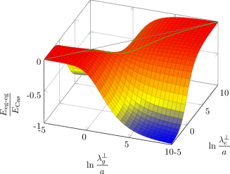
(a) Magneto-electric $\delta$-function plates with $\lambda^{\perp}_{e1}=\lambda^{\perp}_{e2}$ and $\lambda^{\perp}_{g1}=\lambda^{\perp}_{g2}$.

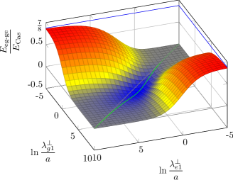
(b) Magneto-electric $\delta$-function plates with $\lambda^{\perp}_{e1}=\lambda^{\perp}_{g2}$ and $\lambda^{\perp}_{g1}=\lambda^{\perp}_{e2}$.

Figure 6: Fractional change in the Casimir energy of parallel magneto-electric $\delta$-function plates separated by distance $a$ relative to the magnitude of the Casimir energy of two perfect electrically conducting parallel plates as a function of the electric and magnetic properties of the $\delta$-function plate, $\ln\frac{\lambda^{\perp}_{e}}{a}$ and $\ln\frac{\lambda^{\perp}_{g}}{a}$, respectively. In 6(a) we assume the magnetic and electric properties of two plates to be same. The interaction energy vanishes when both $\frac{\lambda^{\perp}_{e}}{a}\rightarrow\infty$ and $\frac{\lambda^{\perp}_{g}}{a}\rightarrow\infty$. In 6(b) we assume the two plates have dual properties, i.e., $\lambda^{\perp}_{e1}=\lambda^{\perp}_{g2}$ and $\lambda^{\perp}_{g1}=\lambda^{\perp}_{e2}$. The ratio of energies approaches Boyer’s result for the Casimir energy between a perfect electrically conducting plate and a perfect magnetically conducting plate.

6 Conclusions

In this paper we have extended our investigation of the magneto-electric $\delta$-function plates initiated in [11]. A $\delta$-function plate having both electric and magnetic properties has an interesting property of optically vanishing in the simultaneous perfect electric and perfect magnetic conducting limit, which is a generic property. It can be physically realized in nature by a plasma slab of thickness $d$ in the thin-plate limit, where the characteristic wavenumber $\zeta_{p}=\omega_{p}^{2}d$ satisfies the constraint: $\zeta d\ll\sqrt{\zeta_{p}d}\ll 1$. The Casimir-Polder energy of such a plate with an isotropic atom is always negative when the plate is purely electric and always positive when the plate is purely magnetic. The presence of a magneto-electric $\delta$-function plate on a dielectric medium changes the Casimir-Polder energy by shielding the medium with significant variation observed when the medium is weakly interacting. For the case of interaction between two identical $\delta$-function plates we find that the force is always attractive and vanishes when the plates become simultaneously perfect electric and perfect magnetic conductors. However, if the two $\delta$-function plates have dual properties, i.e., the electric and magnetic properties of one plate are interchanged in the second plate, then the plates can either attract, repel, or experience vanishing force, where latter occurs for a specific set of values of the electric and magnetic properties. It approaches Boyer’s result when one plate becomes a perfect electric conductor and the other plate becomes a perfect magnetic conductor.

- [1] \NAMESommerfeld A., \INMath. Ann.471896317.
- [2] \NAMESommerfeld A., \TITLEMathematical theory of diffraction (Birkhauser, Boston) 2004, [Translators: Nagem R. J., Zampolli M., and Sandri G.].
- [3] \NAMEBoyer T. H., \INPhys. Rev.17419681764.
- [4] \NAMEMilton K. A. \atqueSchwinger J., \TITLEElectromagnetic Radiation: Variational methods, waveguides, and accelerators (Springer, Berlin) 2006.
- [5] \NAMELevin M., McCauley A. P., Rodriguez A. W., Reid M. T. H. \atqueJohnson S. G., \INPhys. Rev. Lett.1052010090403.
- [6] \NAMEBarton G., \INJ. Phys. A: Math. Gen.3720041011.
- [7] \NAMEBarton G., \INJ. Phys. A: Math. Gen.3720043725.
- [8] \NAMEBarton G., \INJ. Phys. A: Math. Gen.37200411945.
- [9] \NAMEBarton G., \INJ. Phys. A: Math. Gen.3820052997.
- [10] \NAMEBarton G., \INJ. Phys. A: Math. Gen.3820053021.
- [11] \NAMEParashar P., Milton K. A., Shajesh K. V. \atqueSchaden M., \INPhys. Rev. D862012085021.
- [12] \NAMEBordag M., Robaschik D. \atqueWieczorek E., \INAnn. Phys.1651985192.
- [13] \NAMEBordag M., Hennig D. \atqueRobaschik D., \INJ. Phys. A: Math. Gen.2519924483.
- [14] \NAMERobaschik D. \atqueWieczorek E., \INAnn. Phys.236199443.
- [15] \NAMEBordag M., \INPhys. Rev. D702004085010.
- [16] \NAMECavero-Pelaez I., Milton K. A., Parashar P. \atqueShajesh K. V., \INPhys. Rev. D782008065018.
- [17] \NAMEKenneth O. \atqueKlich I., \INPhys. Rev. Lett.972006160401.
- [18] \NAMEBoyer T. H., \INPhys. Rev. A919742078.