Quantum 3-SAT is $\text{QMA}_{1}$-Complete

Abstract.

Quantum satisfiability is a constraint satisfaction problem that generalizes classical boolean satisfiability. In the quantum $k$-SAT problem, each constraint is specified by a $k$-local projector and is satisfied by any state in its nullspace. Bravyi showed that quantum $2$-SAT can be solved efficiently on a classical computer and that quantum $k$-SAT with $k\geq 4$ is QMA₁-complete [4]. Quantum $3$-SAT was known to be contained in QMA₁ [4], but its computational hardness was unknown until now. We prove that quantum $3$-SAT is QMA₁-hard, and therefore complete for this complexity class.

1. Introduction

Satisfiability is a widely studied constraint satisfaction problem. In this problem one is given a list of constraints on $n$ boolean variables and asked to determine if there is an $n$-bit string which satisfies each of them. When each constraint involves at most $k$ variables this problem is called $k$-satisfiability, or $k$-SAT. Although $2$-SAT can be solved efficiently on a classical computer, $3$-SAT is NP-complete.

Bravyi introduced a quantum generalization of satisfiability [4]. In the quantum $k$-SAT problem the constraints act on an $n$-qubit Hilbert space and we are asked to determine if there is a state which satisfies all of them. Each constraint is specified by a $k$-local projector and is satisfied by any state in its nullspace.

Bravyi proved that quantum $2$-SAT is in P, quantum $k$-SAT is contained in QMA₁ for any constant $k$, and quantum $k$-SAT for $k\geq 4$ is QMA₁-complete. The computational complexity of quantum $3$-SAT has been an open question. In this paper, we resolve this question by proving that quantum 3-SAT is QMA₁-complete.

Less is known about quantum $k$-SAT than is known about its classical counterpart. Random instances of quantum $k$-SAT have been studied by Laumann et. al. as a function of the clause density $\alpha$ [17, 16]. As in the classical case, it is conjectured that a satisfiability threshold $\alpha_{c}(k)$ exists, above which the probability that a random instance is satisfiable approaches zero as $n\rightarrow\infty$ and below which this probability approaches one [17]. Some bounds on this threshold value have been proven using a quantum version of the Lovász local lemma [3] and by using graph-theoretic techniques [6] but only the case $k=2$ is fully understood [17, 11]. Other previous work has focused on quantum satisfiability with qudit variables of dimension $d>2$ [20, 22, 8, 5] or in restricted geometries [20, 7].

Quantum satisfiability is relevant to the study of frustration-free Hamiltonians. A frustration-free Hamiltonian is a local Hamiltonian (a sum of $k$-local Hermitian operators for some constant $k$) with groundstates that minimize the energy of each local term individually. Such Hamiltonians naturally arise in the study of quantum error correction and play a central role in the field of Hamiltonian complexity, which touches upon condensed matter physics, quantum computation and computational complexity theory [24]. We can view quantum $k$-SAT as the problem where one is asked to determine if a sum of $k$-local projectors is frustration-free, that is to say, if its ground energy is zero.

The computational complexity of quantum $k$-SAT is naturally compared with that of the $k$-Local Hamiltonian problem, which can be viewed as the quantum analogue of MAX $k$-SAT. In this problem one is given a Hamiltonian which is a sum of $k$-local operators, along with constants $a,b$ such that $a<b$. One is asked to determine if the ground energy of the given Hamiltonian is less than $a$ (yes instance) or greater than $b$ (no instance), promised that one of these conditions holds. Note that, for yes instances of this problem, a ground state of the Hamiltonian need not have minimal energy for each $k$-local term; such a system can be frustrated. Because of the possibility of frustration, the $k$-Local Hamiltonian problem can be computationally more difficult than quantum $k$-SAT. Indeed, the $k$-local Hamiltonian problem is QMA-complete for $k\geq 2$ [13]. On the other hand, our result that quantum $3$-SAT is QMA₁-complete shows that these problems are of comparable difficulty for $k\geq 3$ (putting aside the subtle differences between the definitions of QMA and QMA₁).

In the next Section, we provide the basic definitions, describe our results in more detail and give an overview of the remainder of the paper.

2. Definitions and Overview

We first define the complexity class QMA, or Quantum Merlin-Arthur. This class gets its name from a scenario involving Merlin and Arthur, who at the outset are both given an instance of a promise problem encoded as a bit-string $X$. Arthur wishes to know the correct answer to this problem (which is either yes or no) but his time and space resources are bounded as polynomial functions of $|X|$. Merlin has unbounded computational power and can easily obtain the correct answer. Merlin wants to convince Arthur the answer is “yes”, but Arthur doesn’t trust Merlin, so he asks for proof. Merlin hands over an $n$-qubit quantum state $|W\rangle$ (called a witness) that Arthur uses to verify the claim in the following way. He adjoins some number $n_{a}$ of ancilla qubits each in the state $|0\rangle$ to produce

$$|W\rangle|0\rangle^{\otimes n_{a}}$$

(the total number $n+n_{a}$ of qubits in this state must be upper bounded by a polynomial in $|X|$), then applies a polynomial sized verification circuit $U_{X}$ and then measures the first ancilla qubit in the computational basis. If the measurement outcome is $1$, he accepts Merlin’s claim that $X$ is a yes instance. Arthur’s acceptance probability given the state $|W\rangle$ is therefore

$$\text{AP}\left(U_{X},|W\rangle\right)=\left\|\left(\mathbb{I}^{\otimes n}\otimes|1\rangle\langle 1|_{(n+1)}\otimes\mathbb{I}^{\otimes(n_{a}-1)}\right)U_{X}|W\rangle|0\rangle^{\otimes n_{a}}\right\|^{2}.$$ (2.1)

For problems in the class QMA, if Merlin is being truthful he can convince Arthur with probability at least $\frac{2}{3}$. On the other hand, if Merlin is lying (i.e., the answer is actually “no”) then he can only fool Arthur with probability at most $\frac{1}{3}$.

Definition 1 (QMA).

A promise problem $L_{\text{yes}}\cup L_{\text{no}}\subset\{0,1\}^{*}$ is contained in QMA if and only if there exists a uniform polynomial-size quantum circuit family $U_{X}$ such that

If $X\in L_{\text{yes}}$ there exists a state $|W\rangle$ such that $\text{AP}\left(U_{X},|W\rangle\right)\geq\frac{2}{3}$ (completeness).

If $X\in L_{\text{no}}$ then $\text{AP}\left(U_{X},|W\rangle\right)\leq\frac{1}{3}$ for any state $|W\rangle$ (soundness).

As indicated above, the first property is called completeness and the second property soundness. Here we have defined QMA with constant completeness $\frac{2}{3}$ and soundness $\frac{1}{3}$. Kitaev showed that these parameters can be amplified: we obtain an equivalent definition with soundness $2^{-\Omega(|X|^{\alpha})}$ and completeness $1-2^{-\Omega(|X|^{\alpha})}$ for any constant $\alpha$ [14] (see also [18, 23]).

QMA${}_{\text{1}}$ is defined in a similar way to QMA with two modifications. The first is “perfect” completeness – for $X\in L_{\text{yes}}$, Merlin can convince Arthur with probability exactly equal to $1$. The second difference is that Arthur’s verification circuit must consist of a sequence of gates from a fixed universal gate set $\mathcal{G}$. The definition of QMA₁ is not known to be independent of the gate set used. In this paper we use the standard choice

$$\mathcal{G}=\{\widehat{H},T,\text{CNOT}\},$$ (2.2)

where

$$\widehat{H}=\frac{1}{\sqrt{2}}\left(\begin{array}[]{cc}1&1\\ 1&-1\end{array}\right),\quad T=\left(\begin{array}[]{cc}1&0\\ 0&e^{\frac{i\pi}{4}}\end{array}\right),\quad\text{CNOT}=\left(\begin{array}[]{cccc}1&0&0&0\\ 0&1&0&0\\ 0&0&0&1\\ 0&0&1&0\end{array}\right).$$

Definition 2 (QMA${}_{\textbf{1}}$).

A promise problem $L_{\text{yes}}\cup L_{\text{no}}\subset\{0,1\}^{*}$ is contained in QMA${}_{\text{1}}$ if and only if there exists a uniform polynomial-size quantum circuit family $U_{X}$ over the gate set $\mathcal{G}$ such that

If $X\in L_{\text{yes}}$ there exists a state $|W\rangle$ such that $\text{AP}\left(U_{X},|W\rangle\right)=1$ (perfect completeness).

If $X\in L_{\text{no}}$ then $\text{AP}\left(U_{X},|W\rangle\right)\leq\frac{1}{3}$ for any state $|W\rangle$ (soundness).

Just as with QMA, the soundness of a QMA₁ verification procedure (taken to be $\frac{1}{3}$ in the above) can be amplified so that it is very close to zero [14].

Note that we could modify the definition of QMA₁ so that Arthur’s verification procedure may use intermediate measurements in the computational basis as well as operations conditioned on these measurement outcomes. However, expanding the set of allowed verification protocols in this way we obtain an equivalent definition of QMA₁. To see this, note that the controlled version of any unitary written as a product of gates from $\mathcal{G}$ can also be written as a product of gates from $\mathcal{G}$. Given a verification procedure which has some intermediate measurements we can use controlled unitaries in place of all conditional operations. This is the standard trick for deferring measurements until the end of an algorithm; in this case we need not ever measure any of the qubits except the ancilla which gives the output of the computation.

We think of QMA₁ as being very similar to QMA, although the precise relationship between these two classes has yet to be determined. One might expect that QMA$=$QMA₁ since the analogous classical complexity classes MA and MA₁ are known to be equal [25]. This is an interesting open question in quantum complexity theory but we do not explore it further here (see [2, 12, 15] for recent developments). For us, the one-sided error in QMA₁ is primarily an annoyance that prevents the use of standard techniques such as converting between different universal gate sets.

Let us now turn our attention to quantum $3$-SAT. In this problem we are given a Hamiltonian

$$H=\sum_{i=1}^{r}\Pi_{i}$$

that is a sum of $3$-local projectors $\Pi_{i}$ acting on an $n$-qubit Hilbert space. We are promised that either $H$ has ground state energy zero, or else its ground state energy is greater than a constant (which we take without loss of generality to be $1$) and we are asked to decide which is the case.

Note that the matrix elements of a projector $\Pi_{i}$ in an instance of quantum $3$-SAT cannot be specified as arbitrary complex numbers with unlimited precision. In our definition of quantum $3$-SAT we must constrain the set of allowed projectors in some way. One possible choice would be to consider projectors where each matrix element is given to some number of decimal places, but this choice is not well suited to the one-sided error setting we are working in. In particular, it is not clear whether quantum $3$-SAT, defined in this way, is contained in QMA₁ (although it is contained in QMA). On the other hand, if instead we consider projectors where each matrix element is expressed as a rational number with denominator $2^{s}$ (for some fixed integer $s$) then the problem is contained in QMA₁. More generally, let us consider defining quantum $3$-SAT with some set of allowed projectors $\mathcal{P}$. Bravyi proved that quantum $3$-SAT is contained in QMA₁ as long as $\mathcal{P}$ is chosen to satisfy the following condition: there is an efficient algorithm which can be used to measure the eigenvalue of a projector $\Pi\in\mathcal{P}$ in a given state $|\psi\rangle$ using the gate set $\mathcal{G}$ [4, 1]. Of course, since $\mathcal{G}$ is universal, such a measurement can always be approximated using gates from this set, but here we require an exact measurement because of the one-sided error. We discuss this issue in more detail in Appendix A, but we mention this here so the reader is aware of the subtlety. The situation is further complicated by the fact that this technical point was treated incorrectly in reference [4] due to an error in the proof of Lemma 5 [1].

In this work we define quantum $3$-SAT with a restricted set of projectors $\mathcal{P}$ given below. While quantum $3$-SAT remains in QMA₁ for larger classes of projectors, restricting to a smaller set makes our QMA₁-hardness result stronger. The specific set $\mathcal{P}$ that we use arises from technical considerations.

Definition 3.

Let $\mathcal{{P}}$ be the set of $3$-local projectors $\Pi$ which satisfy one of the following two conditions:

1. Every matrix element of $\Pi$ in the computational basis has the form

$$\frac{1}{4}\left(a+i\,b+\sqrt{2}\,c+i\sqrt{2}\,d\right)$$ (2.3)

for $a,b,c,d\in\mathbb{Z}.$

2. There is a $3$-qubit unitary $U$ with matrix elements of the form (2.3) (in the computational basis) such that $U\Pi U^{\dagger}$ is equal to

$$\left(\sqrt{\frac{1}{3}}|000\rangle-\sqrt{\frac{2}{3}}|001\rangle\right)\left(\sqrt{\frac{1}{3}}\langle 000|-\sqrt{\frac{2}{3}}\langle 001|\right)$$

on $3$ of the qubits tensored with the identity on the remaining qubits.

We define quantum $3$-SAT with projectors from $\mathcal{{P}}.$

Definition 4 (Quantum 3-SAT).

Given a collection $\{\Pi_{i}\>:\>i=1,\dots,r\}\subset\mathcal{P}$ of $3$-local projectors acting on $n$ qubits, we are asked to decide if they correspond to a yes instance or a no instance (promised that one is the case), where

Yes: There exists an $n$-qubit state $|\psi\rangle$ satisfying $\Pi_{i}|\psi\rangle=0$ for all $i=1,\dots,r$.

No: $\sum_{i}\langle\psi|\Pi_{i}|\psi\rangle\geq 1$ for all $|\psi\rangle$.

With the definitions given above, we prove that quantum $3$-SAT is QMA₁-complete. In Appendix A we show (following Bravyi [4, 1]) that quantum $3$-SAT is contained in QMA₁. Our main result in this paper is QMA₁-hardness of quantum $3$-SAT. To prove this, we exhibit an efficiently computable mapping from a $g$-gate, $(n+n_{a})$-qubit verification circuit that implements a unitary $U_{X}$ to a Hamiltonian

$$H_{X}=\sum_{i}\Pi_{i,X}$$

which is a sum of $\Theta\left(n_{a}+g\right)$ 3-local projectors $\Pi_{i,X}\in\mathcal{P}$ acting on $\Theta(n+n_{a}+g)$ qubits. Moreover, we prove

Theorem 1 (Completeness).

$H_{X}$ has ground energy $0$ if and only if there exists $|W\rangle$ such that $\text{AP}\left(U_{X},|W\rangle\right)=1,$

and

Theorem 2 (Soundness).

If $\text{AP}\left(U_{X},|W\rangle\right)\leq\frac{1}{3}$ for all $|W\rangle$, then $H_{X}$ has ground energy $\Omega\left(\frac{1}{g^{6}}\right)$.

Note that in our definition of quantum $3$-SAT we require that in the “no” case the ground energy is greater than or equal to $1$, whereas Theorem 2 gives a bound of $\Omega\left(g^{-6}\right)$. To form an instance of quantum $3$-SAT as defined above we repeat each projector $\Pi_{i,X}$ in the instance a suitable number of times (i.e., $\Theta(g^{6})$ times). This shows that any promise problem in QMA₁ can be reduced to quantum $3$-SAT. Since quantum $3$-SAT is also contained in QMA₁ we have proven that it is complete for this complexity class.

Our mapping from the verification circuit $U_{X}$ to the Hamiltonian $H_{X}$ relies on two technical innovations. Like many previous works in the field of Hamiltonian complexity, we use a “clock construction”. In this work we introduce a new one which has some special properties. Most previous QMA- or QMA₁-hardness results use a circuit-to-Hamiltonian mapping which is an immediate and simple application of the clock construction (the standard approach uses a Hilbert space with a computational register and a clock register). In contrast, in this work we define a novel circuit-to-Hamiltonian mapping where the Hamiltonian $H_{X}$ acts on a Hilbert space with a computational register along with two clock registers.

The paper is organized as follows. In Section 3 we introduce our new clock construction. In Section 4 we describe Hamiltonians acting on two clock registers which illustrate the main ideas of our proof that quantum $3$-SAT is QMA₁-hard. Then in Section 5.1 we define the Hamiltonian $H_{X}$ and in Section 5.2 we characterize its zero energy eigenspace, establishing Theorem 1. We prove Theorem 2 in Section 5.3, using a spectral bound due to Kitaev [14].

3. A new clock construction

A clock construction is a local Hamiltonian along with a set of local operators which act on its groundspace in a certain way. It can be used as a set of building blocks to define more complicated Hamiltonians while keeping track of the groundspace. The novel clock construction that we introduce in this Section is a central part of our QMA₁ hardness result. In this Section we focus on the construction itself and discuss its properties. Then in Section 4 we show how to build interesting Hamiltonians using two clock registers. This idea is developed further in Section 5 where we define our circuit-to-Hamiltonian mapping.

In Section 3.1 we give some historical context, in order to motivate the notion of a clock construction. Then in Section 3.2 we summarize the properties of the new one that we introduce in this work. Finally, in Section 3.3 we provide all the details of our construction. On a first read through this paper the reader may wish to skip Section 3.3 since most of our results (with the exception of those presented in Appendix C) are derived using only the properties described in Section 3.2.

3.1. Feynman’s circuit-to-Hamiltonian mapping and Kitaev’s clock construction

Feynman showed how to map a sequence of unitary operators into a Hamiltonian in an interesting way [9]. This mapping is often used to convert statements about quantum circuits into statements about Hamiltonians. Let us start with a quantum circuit $\mathcal{C}$ that acts on $n$ qubits and consists of a product of $m$ one- and two-qubit unitaries

$$W_{m-1}W_{m-2}\dots W_{0}.$$

Now consider a Hilbert space with two registers. The first register holds $n$ qubits and the second register holds an $(m+1)$-level system with orthonormal basis states $|t\rangle$ for $t=0,\dots,m$. Feynman’s Hamiltonian is

$$H_{\text{F}}(\mathcal{C})=\sum_{t=0}^{m-1}\frac{1}{2}\left(\mathbb{I}\otimes|t\rangle\langle t|+\mathbb{I}\otimes|t+1\rangle\langle t+1|-W_{t}^{\dagger}\otimes|t\rangle\langle t+1|-W_{t}\otimes|t+1\rangle\langle t|\right).$$ (3.1)

(Strictly speaking, this definition differs slightly from Feynman’s original Hamiltonian–we have added the first two terms in parentheses). Note that each of the terms in the sum is a projector. Zero eigenvectors of the $t$th term which have all of their support on the clock states $|t\rangle$ and $|t+1\rangle$ have the form

$$|\psi\rangle|t\rangle+W_{t}|\psi\rangle|t+1\rangle$$

where $|\psi\rangle$is an $n$-qubit state. Using this fact, one can show that every state in the zero energy groundspace of $H_{F}^{\text{}}(\mathcal{C})$ is of the form

$$|\text{Hist}_{\text{F}}(\phi)\rangle=\frac{1}{\sqrt{m+1}}\left(|\phi\rangle|0\rangle+\sum_{t=1}^{m}W_{t-1}W_{t-2}\dots W_{0}|\phi\rangle|t\rangle\right)$$

where $|\phi\rangle$ is an $n$-qubit state. The state $|\text{Hist}_{\text{F}}\mbox{($\phi$)}\rangle$ is sometimes called a history state because it contains every intermediate state $W_{t-1}W_{t-2}\dots W_{0}|\phi\rangle$ obtained during the course of applying the circuit $\mathcal{C}$ to the initial state $|\phi\rangle.$ The second register is called the clock register and keeps track of the number of unitaries that have been applied.

The clock register in Feynman’s construction is an $(m+1)$-level system. However, Kitaev noticed that a modification of Feynman’s idea can be used to map the circuit $\mathcal{C}$ into a local Hamiltonian acting on a system made only from qubits. Again the Hilbert space has two registers; the first holds $n$ qubits as before but now the second register has $m$ qubits. The idea is to encode Feynman’s $m+1$ clock states as $m$-bit unary strings

$$|t\rangle_{\text{u}}=|\underbrace{1\cdots 1}_{t}\underbrace{0\cdots 0}_{m-t}\rangle.$$

The $(m+1)$-dimensional span of these clock states is called the clock subspace. It is the groundspace of the 2-local, $m$-qubit Hamiltonian

$$H_{\text{unary}}^{(m)}=\sum_{i=1}^{m-1}|01\rangle\langle 01|_{i,i+1}.$$

This is the first part of Kitaev’s clock construction: a local Hamiltonian acting on a system of qubits which has the desired number of groundstates. The second part of the clock construction is a set of local operators which act in a special way on states that have all of their support in the clock subspace. For any unitary $U$ acting on the first register, define projectors

$$h_{t,t+1}^{\text{u}}(U)=\frac{1}{2} \left(\mathbb{I}\otimes|100\rangle\langle 100|_{t,t+1,t+2}+\mathbb{I}\otimes|110\rangle\langle 110|_{t,t+1,t+2}\right)$$ (3.2)

$$-\frac{1}{2} \left(U^{\dagger}\otimes|100\rangle\langle 110|_{t,t+1,t+2}+U\otimes|110\rangle\langle 100|_{t,t+1,t+2}\right).$$

These are called the transition operators for the clock. Note that on the LHS of this expression the subscript labels the operator, whereas on the RHS the subscript indicates which qubits the operator acts on nontrivially. Writing $\Pi_{\text{unary}}^{(m)}$ for the projector onto the clock subspace, we have

$$\left(\mathbb{I}\otimes\Pi_{\text{unary}}^{(m)}\right)h_{t,t+1}^{\text{u}}(U)\left(\mathbb{I}\otimes\Pi_{\text{unary}}^{(m)}\right)= \frac{1}{2}\left(\mathbb{I}\otimes|t\rangle\langle t|_{\text{u}}+\mathbb{I}\otimes|t+1\rangle\langle t+1|_{\text{u}}\right)$$ (3.3)

$$- \frac{1}{2}\left(U^{\dagger}\otimes|t\rangle\langle t+1|_{\text{u}}+U\otimes|t+1\rangle\langle t|_{\text{u}}\right),$$

which should be compared with (3.1). Kitaev’s Hamiltonian is

$$H_{\text{K}}(\mathcal{C})=\mathbb{I}\otimes H_{\text{unary}}^{(m)}+\sum_{t=0}^{m-1}h_{t,t+1}^{\text{u}}(W_{t})$$ (3.4)

Since both terms in (3.4) are positive semidefinite, every state in its zero energy groundspace is a zero eigenvector of the first term. Within the nullspace of $\mathbb{I}\otimes H_{\text{unary}}^{(m)}$, $H_{K}(\mathcal{C})$ acts in the same way as $H_{\text{F}}(\mathcal{C})$. Thus, every state in the groundspace of (3.4) is a history state

$$\frac{1}{\sqrt{m+1}}\left(|\phi\rangle|0\rangle_{\text{u}}+\sum_{t=1}^{m}W_{t-1}W_{t-2}\dots W_{0}|\phi\rangle|t\rangle_{\text{u}}\right)$$

for some $n$-qubit state $|\phi\rangle.$ Furthermore, the Hamiltonian $H_{\text{K}}(\mathcal{C})$ is $5$-local since each unitary $W_{j}$ is either one- or two-local. This circuit-to-Hamiltonian mapping was used by Kitaev in his proof that $5$-local Hamiltonian is QMA-complete [14].

Let us now view Kitaev’s clock construction as a mathematical object of independent interest. In our view, the clock construction is specified by the Hamiltonian $H_{\text{unary}}^{(m)}$ along with the transition operators $h_{t,t+1}^{\text{u}}(U)$ which act as in equation (3.3). This is the set of operators which Kitaev used to instantiate Feynman’s Hamiltonian as a $5$-local Hamiltonian acting on a system of qubits. In Kitaev’s construction the Hamiltonian $H_{\text{unary}}^{(m)}$ is a sum of 2-local projectors and the transition operators are $(k+3)$-local projectors where $k$ is the locality of the unitary $U$. In contrast, in this Section we introduce a clock construction where the clock states are groundstates of a Hamiltonian that is a sum of 3-local projectors and where the transition operators are $\left(k+2\right)$-local projectors. If we naïvely replace Kitaev’s clock construction with ours, it allows us to instantiate Feynman’s Hamiltonian as a $4$-local Hamiltonian. This is not good enough for our purposes since we are interested in quantum $3$-SAT where the projector terms are $3$-local. The circuit-to-Hamiltonian mapping that we define in this paper is not based on Feynman’s Hamiltonian, and in particular only ever uses the transition operators $h_{t,t+1}^{\text{u}}(U)$ for single-qubit unitaries $U$. Nevertheless we are able to encode a computation consisting of $1$- and $2$-qubit gates in the ground state of the resulting Hamiltonian. This nontrivial fact is one of the main contributions of our paper, and is the subject of Sections 4 and 5.

3.2. Summary of the new clock construction

Our construction, including explicit expressions for all the operators mentioned below, is presented in full detail in Section 3.3. Here we summarize its features. As discussed above, the crucial difference between our clock construction and Kitaev’s is the locality of the transition operators.

For any $N\in\{2,3,\dots\}$, we present a Hamiltonian

$$H_{\text{clock}}^{(N)}$$

which acts on the Hilbert space

$$\mathcal{H}_{\text{clock}}^{(N)}=\left(\mathbb{C}^{2}\right)^{7N-3}$$ (3.5)

of $7N-3$ qubits and which is a sum of 3-local projectors from the set $\mathcal{{P}}$ given in Definition 3. The zero energy groundspace of $H_{\text{clock}}^{(N)}$ is spanned by orthonormal states

$$|C_{i}\rangle,\quad i=1,\dots,N.$$

Now let $\mathcal{H}_{\text{comp}}$ be a computational register containing some (arbitrary) number of qubits, and let $U$ be a unitary acting on this register. We exhibit projectors

$$h_{i,i+1}(U)$$

for $i=1,\dots,N-1,$ which act on

$$\mathcal{H}_{\text{comp}}\otimes\mathcal{H}_{\text{clock }}^{(N)}.$$

These are the transition operators (3.3) for the clock. Specifically, they satisfy

$$\left(\mathbb{I}\otimes\Pi_{\text{clock}}^{(N)}\right)h_{i,i+1}(U)\left(\mathbb{I}\otimes\Pi_{\text{clock}}^{(N)}\right)= \frac{1}{8}\left(\mathbb{I}\otimes|C_{i}\rangle\langle C_{i}|+\mathbb{I}\otimes|C_{i+1}\rangle\langle C_{i+1}|\right)$$

$$- \frac{1}{8}\left(U^{\dagger}\otimes|C_{i}\rangle\langle C_{i+1}|+U\otimes|C_{i+1}\rangle\langle C_{i}|\right),$$ (3.6)

where $\Pi_{\text{clock}}^{(N)}=\sum_{i=1}^{N}|C_{i}\rangle\langle C_{i}|$ projects onto the clock subspace. Comparing these operators with Kitaev’s, we see that the prefactor of $\frac{1}{2}$ in (3.3) has been replaced with $\frac{1}{8}$ in (3.6). For our purposes only the nullspaces of these operators are relevant, and this prefactor does not affect the null space.

A much more important difference is the locality. In our case, the operator $h_{i,i+1}(U)$ is a $(k+2)$-local projector where $k$ is the locality of the unitary $U$. When $U$ is the identity the projector $h_{i,i+1}(1)$ acts nontrivially only on two qubits of $\mathcal{H}_{\text{clock }}^{(N)}$ and we write

$$h_{i,i+1}\doteq h_{i,i+1}(\mathbb{I}).$$

Thus, for a single-qubit unitary, $h_{i,i+1}(U)$ is only 3-local (in contrast with Kitaev’s clock where $h_{i,i+1}^{\text{u}}(U)$ would be $4$-local). Our circuit-to-Hamiltonian mapping, presented in Sections 4 and 5 exploits this feature (it is partly inspired by the railroad switch idea from [21]).

Finally, we also exhibit 1-local (single-qubit) projectors

$$C_{\geq i}\qquad\text{and}\qquad C_{\leq i}$$ (3.7)

for $i=1,\dots,N$, whose role is to “pick out” clock states $|C_{j}\rangle$ with $j\geq i$ or $j\leq i$ respectively. They act on the Hilbert space (3.5) of the clock and satisfy

$$\Pi_{\text{clock}}^{(N)}C_{\geq i}\Pi_{\text{clock}}^{(N)} =\frac{1}{2}|C_{i}\rangle\langle C_{i}|+\sum_{i<j\leq N}|C_{j}\rangle\langle C_{j}|$$ (3.8)

$$\Pi_{\text{clock}}^{(N)}C_{\leq i}\Pi_{\text{clock}}^{(N)} =\sum_{1\leq j<i}|C_{j}\rangle\langle C_{j}|+\frac{1}{2}|C_{i}\rangle\langle C_{i}|$$ (3.9)

with the understanding that when $i=1$ the first term in (3.9) is zero and when $i=N$ the second term in (3.8) is zero. As in (3.6), only the nullspaces of the operators on the RHS of (3.8) and (3.9) are important for our purposes. In particular, it is not significant that the $|C_{i}\rangle\langle C_{i}|$ terms have different prefactors, since the (positive) value of these coefficients do not affect the nullspace.

3.3. Details of the new clock construction

Here we present the details of the clock construction described in Section 3.2. The reader may safely skip this Section on a first read through this paper. Subsequent Sections can be understood using the summary presented in Section 3.2.

Our goal is to define $H_{\text{clock}}^{(N)}$ along with the operators $C_{\geq i},C_{\leq i},h_{i,i+1}(U)$ satisfying the properties specified in Section 3.2. We present our construction in two steps. First, we define a Hamiltonian $H_{\text{triplet}}^{(2N)}$ that we call the “triplet” Hamiltonian. It already has many (but not all) of the properties that we desire for our clock construction. In the second step, we construct $H_{\text{clock}}^{(N)}$ from the “triplet” Hamiltonian by appending another register and adding terms which act between the two registers.

Let $N\in\{2,3,4,\dots\}$. We now define the triplet Hamiltonian $H_{\text{triplet}}^{(2N)}$ which is a sum of 3-local projectors and acts on the Hilbert space of $3(2N-1)$ qubits:

$$H_{\text{triplet}}^{(2N)}=H_{1}+H_{2}+H_{3},$$ (3.10)

where

$$H_{1} =\sum_{i=0}^{2N-2}\left(|111\rangle\langle 111|+|010\rangle\langle 010|+|001\rangle\langle 001|+|\theta^{-}\rangle\langle\theta^{-}|\right)_{3i+1,3i+2,3i+3}$$ (3.11)

$$+|000\rangle\langle 000|_{123}+\left(|100\rangle\langle 100|+|011\rangle\langle 011|\right)_{3(2N-2)+1,3(2N-2)+2,3(2N-2)+3},$$

$$H_{2} =\sum_{i=0}^{2N-3}\left(|10\rangle\langle 10|+|01\rangle\langle 01|\right)_{3i+2,3i+3}\otimes\left(|1\rangle\langle 1|_{3i+4}+|1\rangle\langle 1|_{3i+5}+|1\rangle\langle 1|_{3i+6}\right)$$ (3.12)

$$+\sum_{i=0}^{2N-3}|00\rangle\langle 00|_{3i+1,3i+2}\otimes\left(|1\rangle\langle 1|_{3i+4}+|1\rangle\langle 1|_{3i+5}+|1\rangle\langle 1|_{3i+6}\right),$$

$$H_{3} =\sum_{i=0}^{2N-3}|\gamma\rangle\langle\gamma|_{3i+3,3i+4,3i+5}$$ (3.13)

act on triplets of qubits as in Figure 3.1, with $|\theta^{\pm}\rangle$ and $|\gamma\rangle$ given by

$$|\theta^{\pm}\rangle =\frac{1}{\sqrt{2}}\left(|100\rangle\pm|011\rangle\right),\qquad|\gamma\rangle=\frac{1}{\sqrt{3}}|100\rangle-\sqrt{\frac{2}{3}}|011\rangle.$$

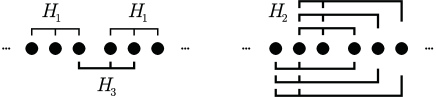
Figure 3.1. The terms $H_{1}$, $H_{2}$ and $H_{3}$ in the Hamiltonian $H_{\text{triplet}}^{(2N)}$ (3.10) involve consecutive triplets of qubits.

We now construct $2N$ orthonormal basis states which span the ground space of $H_{\text{triplet}}^{(2N)}$. First, consider $H_{1}.$ Observe that the groundspace of $H_{1}$ is spanned by the set of all products of three qubit states of the form

$$|\chi_{1}\rangle|\chi_{2}\rangle\dots|\chi_{2N-1}\rangle,$$

where

$$|\chi_{1}\rangle \in\{|110\rangle,|101\rangle,|\theta^{+}\rangle\},$$

$$|\chi_{j}\rangle \in\{|000\rangle,|110\rangle,|101\rangle,|\theta^{+}\rangle\}\;\text{for}\;j=2,\dots,2N-2,$$

$$|\chi_{2N-1}\rangle \in\{|000\rangle,|110\rangle,|101\rangle\}.$$

Let us now consider the action of $H_{2}$ on the groundspace of $H_{1}$. The terms in $H_{2}$ assign an energy penalty to certain products of three qubit states. The first term penalizes any state where $|\chi_{i}\rangle\in\{|110\rangle,|101\rangle\}$ but $|\chi_{i+1}\rangle\neq|000\rangle.$ The second term penalizes states where $|\chi_{i}\rangle=|000\rangle$ but $|\chi_{i+1}\rangle\neq|000\rangle.$ The projector onto the zero energy groundspace of $H_{1}+H_{2}$ is therefore given by

$$\Pi_{12}=\sum_{i=1}^{4N-2}|\hat{i}\rangle\langle\hat{i}|+\sum_{k=1}^{2N-2}|\tilde{k}\rangle\langle\tilde{k}|,$$ (3.14)

where

$$|\widehat{1}\rangle =|110\rangle|000\rangle|000\rangle\dots|000\rangle,$$ (3.15)

$$|\widehat{2}\rangle =|101\rangle|000\rangle|000\rangle\dots|000\rangle$$

$$|\widehat{3}\rangle =|\theta^{+}\rangle\;|110\rangle|000\rangle\dots|000\rangle,$$

$$|\widehat{4}\rangle =|\theta^{+}\rangle\;|101\rangle|000\rangle\dots|000\rangle,$$

$$\;\,\vdots$$

$$|\widehat{4N-3}\rangle =|\theta^{+}\rangle\,|\theta^{+}\rangle\;\dots\;|\theta^{+}\rangle\;|110\rangle,$$

$$|\widehat{4N-2}\rangle =|\theta^{+}\rangle\;|\theta^{+}\rangle\;\dots\;|\theta^{+}\rangle\;|101\rangle$$ (3.16)

and

$$|\tilde{k}\rangle=|\theta^{+}\rangle^{\otimes k}|000\rangle^{\otimes 2N-1-k}$$ (3.17)

for $k=1,\dots,2N-2$. Note that the states $|\widehat{i}\rangle$ each contain an “active” triplet $|110\rangle$ or $|101\rangle$ separating $|\theta^{+}\rangle$ to the left and $|000\rangle$ to the right. In contrast, the states $|\tilde{k}\rangle$ do not have an active triplet separating the two regions.

The role of $H_{3}$ is twofold. It assigns an energy penalty to each of the states $\{|\tilde{k}\rangle\}$ and to certain linear combinations of the states $\{|\hat{i}\rangle\}$. This can be seen by looking at the restriction of $H_{3}$ to the groundspace of $H_{1}+H_{2}$,

$$\Pi_{12}H_{3}\Pi_{12}=\frac{1}{3}\sum_{i=2}^{2N-1}\left(|\widehat{2i-2}\rangle-|\widehat{2i-1}\rangle\right)\left(\langle\widehat{2i-2}|-\langle\widehat{2i-1}|\right)+\frac{1}{6}\sum_{k=1}^{2N-2}|\tilde{k}\rangle\langle\tilde{k}|.$$ (3.18)

We are now able to fully characterize the zero energy groundspace of $H_{\text{triplet}}^{(2N)}$. It is spanned by the $2N$ states

$$|c_{1}\rangle =|\widehat{1}\rangle,$$ (3.19)

$$|c_{i}\rangle =\frac{1}{\sqrt{2}}\left(|\widehat{2i-2}\rangle+|\widehat{2i-1}\rangle\right)\;\text{for}\;i=2,\dots,2N-1,$$ (3.20)

$$|c_{2N}\rangle =|\widehat{4N-2}\rangle.$$ (3.21)

We now consider some local operators and their actions in the zero energy subspace of $H_{\text{triplet}}^{(2N)}.$ We will see that they have properties similar to those described in Section 3.2.

Define $2$-local projectors

$$q_{1} =|10\rangle\langle 10|_{23},$$

$$q_{i} =|01\rangle\langle 01|_{3i-4,3i-3}\;\text{for}\;i=2,\dots,2N,$$ (3.22)

and note that, projected to the groundspace of $H_{\text{triplet}}^{(2N)}$, we have

$$\Pi^{(2N)}q_{i}\Pi^{(2N)}=\alpha_{i}|c_{i}\rangle\langle c_{i}|,$$ (3.23)

where $\Pi^{(2N)}=\sum_{i=1}^{2N}|c_{i}\rangle\langle c_{i}|$ and

$$\alpha_{i}=\begin{cases}1,&\text{ if }i\in\{1,2N\}\\ \frac{1}{2},&\text{ otherwise. }\end{cases}$$ (3.24)

Now adjoin another register so the Hilbert space is

$$\mathcal{H}_{\text{comp}}\otimes\left(\mathbb{C}^{2}\right)^{6N-3}$$

and let $U$ be a unitary acting on $\mathcal{H}_{\text{comp}}$. Define

$$g_{i,i+1}(U)= \frac{1}{\alpha_{i}+\alpha_{i+1}}\left(\alpha_{i+1}\,\mathbb{I}\otimes|10\rangle\langle 10|_{3i-1,3i}+\alpha_{i}\,\mathbb{I}\otimes|01\rangle\langle 01|_{3i-1,3i}\right)$$ (3.25)

$$- \frac{\sqrt{\alpha_{i+1}\alpha_{i}}}{\alpha_{i}+\alpha_{i+1}}\left(U^{\dagger}\otimes|10\rangle\langle 01|_{3i-1,3i}+U\otimes|01\rangle\langle 10|_{3i-1,3i}\right)$$

for $i=1,\dots,2N-1$. Note that $g_{i,i+1}(U)$ is a $(k+2)$-local projector if $U$ is a $k$-qubit unitary, and furthermore

$$\left(\mathbb{I}\otimes\Pi^{(2N)}\right)g_{i,i+1}(U)\left(\mathbb{I}\otimes\Pi^{(2N)}\right) =\beta_{i}\left(\mathbb{I}\otimes|c_{i}\rangle\langle c_{i}|+\mathbb{I}\otimes|c_{i+1}\rangle\langle c_{i+1}|\right)$$

$$-\beta_{i}\left(U^{\dagger}\otimes|c_{i}\rangle\langle c_{i+1}|+U\otimes|c_{i+1}\rangle\langle c_{i}|\right),$$ (3.26)

where

$$\beta_{i}=\frac{\alpha_{i+1}\alpha_{i}}{\alpha_{i}+\alpha_{i+1}}=\begin{cases}\frac{1}{3},&\text{ if }i\in\{1,2N-1\},\\ \frac{1}{4},&\text{ otherwise.}\end{cases}$$ (3.27)

Equation (3.26) should be compared to (3.6).

Now we are ready to define $H_{\text{clock}}^{(N)}$ and the associated operators which make up our clock construction. Consider the Hilbert space

$$\left(\mathbb{C}^{2}\right)^{6N-3}\otimes\left(\mathbb{C}^{2}\right)^{N}$$

and the Hamiltonian

$$H_{\text{clock}}^{(N)}=H_{\text{triplet}}^{(2N)}\otimes\mathbb{I}+\mathbb{I}\otimes H_{\text{unary}}^{(N)}+H_{\text{sync}}+\sum_{i=1}^{N}g_{2i-1,2i}(\sigma_{i}^{x}),$$ (3.28)

where $\sigma_{i}^{x}$ is the $\sigma^{x}$ operator acting on the $i$th qubit of the second register. Observe that each operator $g_{2i-1,2i}(\sigma_{i}^{x})$ (defined through (3.25)) is a 3-local projector which acts on qubits $6i-4$ and $6i-5$ of the first register and qubit $i$ of the second register. $H_{\text{unary}}^{(N)}$ acts on the second register as

$$H_{\text{unary}}^{(N)}=\sum_{i=1}^{N-1}|01\rangle\langle 01|_{i,i+1}$$ (3.29)

and its ground state subspace is spanned by the unary states

$$|t\rangle_{\text{u}}=|\underbrace{1\cdots 1}_{t}\underbrace{0\cdots 0}_{N-t}\rangle.$$ (3.30)

The Hamiltonian $H_{\text{sync}}$ acts on both registers as

$$H_{\text{sync}}=q_{1}\otimes|1\rangle\langle 1|_{1}+\sum_{j=2}^{2N-1}q_{j}\otimes\left(|0\rangle\langle 0|_{\left\lfloor\frac{j}{2}\right\rfloor}+|1\rangle\langle 1|_{\left\lfloor\frac{j}{2}\right\rfloor+1}\right)+q_{2N}\otimes|0\rangle\langle 0|_{N}.$$ (3.31)

where $q_{j}$ is defined in (3.22) and $\left\lfloor\cdot\right\rfloor$ is the floor function. Here the tensor product separates the first $6N-3$ qubits from the last $N$ qubits.

The zero energy groundspace of $H_{\text{triplet}}^{(2N)}\otimes\mathbb{I}+\mathbb{I}\otimes H_{\text{unary}}^{(N)}+H_{\text{sync}}$ is spanned by the states

$$|e_{j}\rangle=|c_{j}\rangle\left|\left\lfloor j/2\right\rfloor\right\rangle_{\text{u}}$$ (3.32)

for $j=1,\dots,2N$, where $|c_{j}\rangle$ are the ground states of $H_{\text{triplet}}^{(2N)}$ as defined in equations (3.19)-(3.21). Let $\Pi_{e}^{(2N)}$ be the projector onto the subspace spanned by $\{|e_{j}\rangle\}$. The last term in (3.28), the operator $\sum_{i}g_{2i-1,2i}(\sigma_{i}^{x})$, acts within this space as

$$\Pi_{\text{e}}^{(2N)}\left(\sum_{i=1}^{N}g_{2i-1,2i}(\sigma_{i}^{x})\right)\Pi_{e}^{(2N)}=\sum_{i=1}^{N}\beta_{2i-1}\left(|e_{2i-1}\rangle-|e_{2i}\rangle\right)\left(\langle e_{2i-1}|-\langle e_{2i}|\right)$$ (3.33)

where $\beta_{i}$ is defined in (3.27). Taking linear combinations of the states (3.32) which are zero eigenvectors of (3.33), we finally get a spanning set of zero energy groundstates for $H_{\text{clock}}^{(N)}$:

$$|C_{i}\rangle =\frac{1}{\sqrt{2}}\big{(}|c_{2i-1}\rangle|i-1\rangle_{\text{u}}+|c_{2i}\rangle|i\rangle_{\text{u}}\big{)}$$ (3.34)

$$=\frac{1}{\sqrt{2}}\big{(}|c_{2i-1}\rangle|\underbrace{1\cdots 1}_{i-1}\underbrace{0\cdots 0}_{N-i+1}\rangle+|c_{2i}\rangle|\underbrace{1\cdots 1}_{i}\underbrace{0\cdots 0}_{N-i}\rangle\big{)}$$ (3.35)

for $i=1,\dots,N.$ As an example, we expand these states in the computational basis for $N=4$ in Figure B.1 in Appendix B.

We now define the operators

$$C_{\leq i} =\mathbb{I}\otimes|0\rangle\langle 0|_{i},$$ (3.36)

$$C_{\geq i} =\mathbb{I}\otimes|1\rangle\langle 1|_{i},$$ (3.37)

which act on the $i$th qubit of the second register, for $i=1,\dots,N$. Using (3.35) it is easy to verify that these operators satisfy (3.8) and (3.9) as claimed in Section 3.2.

Finally, we are ready to define the transition operators $h_{i,i+1}(U)$ and to show that they satisfy (3.6). We consider a Hilbert space

$$\mathcal{H}_{\text{comp}}\otimes\mathcal{H}_{\text{clock}}^{(N)}=\mathcal{H}_{\text{comp}}\otimes\left(\mathbb{C}^{2}\right)^{6N-3}\otimes\left(\mathbb{C}^{2}\right)^{N}$$

and a unitary $U$ which acts on $\mathcal{H}_{\text{comp}}$. Define

$$h_{i,i+1}(U)=g_{2i,2i+1}(U)\otimes\mathbb{I}$$ (3.38)

for $i=1,\dots,N-1.$ Here $g_{2i,2i+1}(U)$ acts on the computational register and two out of the $6N-3$ qubits in the second register. Note that $h_{i,i+1}(U)$ is a $(k+2)$-local projector when $U$ is a $k$-qubit unitary. Using equations (3.38), (3.35), (3.26) and the fact that $\beta_{2i}=\frac{1}{4}$ for all $i=1,\dots,N-1$ we confirm (3.6):

$$\left(\mathbb{I}\otimes\Pi_{\text{clock}}^{(N)}\right)h_{i,i+1}(U)\left(\mathbb{I}\otimes\Pi_{\text{clock}}^{(N)}\right) =\frac{1}{8}\left(\mathbb{I}\otimes|C_{i}\rangle\langle C_{i}|+\mathbb{I}\otimes|C_{i+1}\rangle\langle C_{i+1}|\right)$$

$$-\frac{1}{8}\left(U^{\dagger}\otimes|C_{i}\rangle\langle C_{i+1}|+U\otimes|C_{i+1}\rangle\langle C_{i}|\right).$$

We can also write an explicit expression for $h_{i,i+1}(U)$ using (3.25) and the fact that $\alpha_{2i}=\alpha_{2i+1}=\frac{1}{2}$ for all $i=1,\dots,N-1$:

$$h_{i,i+1}(U) =\frac{1}{2}\left(\mathbb{I}\otimes|10\rangle\langle 10|_{6i-1,6i}\otimes\mathbb{I}+\mathbb{I}\otimes|01\rangle\langle 01|_{6i-1,6i}\otimes\mathbb{I}\right)$$

$$-\frac{1}{2}\left(U^{\dagger}\otimes|10\rangle\langle 01|_{6i-1,6i}\otimes\mathbb{I}+U\otimes|01\rangle\langle 10|_{6i-1,6i}\otimes\mathbb{I}\right).$$ (3.39)

Finally, note that $H_{\text{clock}}^{(N)}$ is a sum of 3-local projectors. We now show that each of the projectors in the sum is from the set $\mathcal{P}$ given in Definition 3. Looking at equations (3.11)-(3.13) we see that $H_{\text{triplet}}^{(2N)}$ is a sum of projectors which are diagonal in the computational basis (and which satisfy condition 1 in Definition 3) along with projectors of the form $|\theta^{-}\rangle\langle\theta^{-}|$ (which satisfy condition 1 in Definition 3) and projectors of the form $|\gamma\rangle\langle\gamma|$ (which satisfy condition 2). $H_{\text{unary}}^{(N)}$ and $H_{\text{sync}}$ are sums of classical projectors which satisfy condition 1. Now consider the terms $g_{2i-1,2i}(\sigma_{i}^{x})$ for $i=1,\dots,N$. Looking at equations (3.24) and (3.25) we see that, for $i\in\{2,\dots,N-1\}$ each of these terms is a projector which satisfies condition 1. We consider the terms with $i=1$ and $i=N$ separately. First, look at $g_{1,2}(\sigma_{1}^{x})$ which acts on qubits $2$ and $3$ of the first register and qubit $1$ of the second register as

$$\frac{1}{3}\left(|10\rangle\langle 10|\otimes\mathbb{I}+2\,|01\rangle\langle 01|\otimes\mathbb{I}-\sqrt{2}\,|10\rangle\langle 01|\otimes\sigma_{x}-\sqrt{2}\,|01\rangle\langle 10|\otimes\sigma_{x}\right)$$

$$= \frac{1}{3}\left(|10\rangle\langle 10|+2\,|01\rangle\langle 01|-\sqrt{2}\,|10\rangle\langle 01|-\sqrt{2}\,|01\rangle\langle 10|\right)\otimes|+\rangle\langle+|$$

$$+ \frac{1}{3}\left(|10\rangle\langle 10|+2\,|01\rangle\langle 01|+\sqrt{2}\,|10\rangle\langle 01|+\sqrt{2}\,|01\rangle\langle 10|\right)\otimes|-\rangle\langle-|$$

where $|+\rangle$ and $|-\rangle$ are the eigenstates of the Pauli $\sigma^{x}$ operator. It is not hard to see that each of the two terms on the RHS of this equation is a projector which satisfies condition 2 from Definition 3. A similar decomposition can be used to write $g_{2N-1,2N}(\sigma_{N}^{x})$ as a sum of two projectors satisfying condition 2.

This completes our description of the clock construction with the properties outlined in Section 3.2.

4. Hamiltonians acting on two clock registers

Here we develop the main ideas behind our circuit-to-Hamiltonian mapping, using the new clock construction described in the previous section. A key feature of our approach is that we use two clock registers, with Hilbert space

$$\mathcal{H}_{\text{clock}}^{(N)}\otimes\mathcal{H}_{\text{clock}}^{(N)}.$$ (4.1)

Let’s consider some local operators which act on this space. The Hamiltonians

$$\mathbb{I}\otimes H_{\text{clock}}^{(N)}\qquad\text{and}\qquad H_{\text{clock}}^{(N)}\otimes\mathbb{I}$$

are both sums of 3-local projectors as discussed in the previous section. Since $C_{\leq i}$ and $C_{\geq i}$ are 1-local projectors, we can form 2-local projectors by taking tensor products, e.g.,

$$C_{\leq i}\otimes C_{\geq j}.$$

Similarly, since the operators $h_{k,k+1}$ are 2-local projectors, terms such as

$$h_{k,k+1}\otimes C_{\leq i}$$

are 3-local projectors. For convenience and to ease notation later on, we define the following sum of such terms

$$S^{(k,k+2)} =C_{\leq k}\otimes C_{\geq(k+2)}+h_{k,k+1}\otimes C_{\leq(k+1)}+h_{(k+1),(k+2)}\otimes C_{\geq(k+1)}$$ (4.2)

$$+C_{\geq(k+2)}\otimes C_{\leq k}+C_{\leq(k+1)}\otimes h_{k,k+1}+C_{\geq(k+1)}\otimes h_{(k+1),(k+2)}$$

for $k=1,\dots,N-2.$

We begin by looking at a simple Hamiltonian which acts in the Hilbert space (4.1); this example introduces some notation and conventions that we use later on. We then consider two examples where the Hilbert space (4.1) is tensored with a computational register. These examples contain the essential ideas behind our proof in Section 5 that quantum $3$-SAT is QMA₁-hard.

4.1. Warm up example

As a warm-up, consider the following Hamiltonian acting on the space (4.1) with $N=9$:

$$\mathbb{I}\otimes H_{\text{clock}}^{(9)}+H_{\text{clock}}^{(9)}\otimes\mathbb{I}+S^{(4,6)},$$ (4.3)

with $S^{(4,6)}$ given by (4.2). We will see how the zero energy groundspace of this operator can be represented pictorially.

Recall (from Section 3.2) that $H_{\text{clock}}^{(9)}$ has $9$ orthonormal zero energy states $|C_{i}\rangle$ for $i=1,\dots,9$. The first two terms of (4.3)

$$\mathbb{I}\otimes H_{\text{clock}}^{(9)}+H_{\text{clock}}^{(9)}\otimes\mathbb{I}$$ (4.4)

therefore have 81 zero energy ground states which we choose to represent as a set of vertices arranged in a 2D grid, as shown in Figure 4.1(a). We adopt the convention that the vertex in the top left corner has coordinates $(i,j)=(1,1)$, the $i$ coordinate increases moving to the right and the $j$ coordinate increases moving downwards. The vertex with coordinate $(i,j)$ is associated with the groundstate $|C_{i}\rangle|C_{j}\rangle.$

We add $S^{(4,6)}$ to (4.4) a few terms at a time. First look at

$$\mathbb{I}\otimes H_{\text{clock}}^{(9)}+H_{\text{clock}}^{(9)}\otimes\mathbb{I}+C{}_{\leq 4}\otimes C_{\geq 6}+C_{\geq 6}\otimes C_{\leq 4}$$

which is just the first two terms of $S^{(4,6)}$ added to (4.4). Using the expressions (3.8) and (3.9) we see that adding this term assigns an energy penalty to all the states $|C_{i}\rangle|C_{j}\rangle$ with either $i\leq 4$ and $j\geq 6$ or $i\geq 6$ and $j\leq 4$. Eliminating the corresponding vertices from Figure 4.1(a) we get Figure 4.1(b).

Now look at the next term which is $h_{4,5}\otimes C_{\leq 5}$. Using equations (3.6) and (3.36) we get

$$\left(\Pi_{\text{clock}}^{(9)}\otimes\Pi_{\text{clock}}^{(9)}\right) \left(h_{4,5}\otimes C_{\leq 5}\right)\left(\Pi_{\text{clock}}^{(9)}\otimes\Pi_{\text{clock}}^{(9)}\right)$$

$$=\frac{1}{8}\left(|C_{4}\rangle-|C_{5}\rangle\right)\left(\langle C_{4}|-\langle C_{5}|\right)\otimes\sum_{j=1}^{5}\left(1-\frac{1}{2}\delta_{j,5}\right)|C_{j}\rangle\langle C_{j}|.$$

From this we see that states $|C_{4}\rangle|C_{j}\rangle$ and $|C_{5}\rangle|C_{j}\rangle$ for $j=1,\dots,5$ are not zero energy states for this term although their uniform superpositions $\frac{1}{\sqrt{2}}\left(|C_{4}\rangle+|C_{5}\rangle\right)|C_{j}\rangle$ are. We represent the groundspace of

$$\mathbb{I}\otimes H_{\text{clock}}^{(9)}+H_{\text{clock}}^{(9)}\otimes\mathbb{I}+C{}_{\leq 4}\otimes C_{\geq 6}+C_{\geq 6}\otimes C_{\leq 4}+h_{4,5}\otimes C_{\leq 5}$$

as the graph in Figure 4.1(c), where now ground states are in one-to-one correspondence with the connected components of the graph. The ground state corresponding to a given connected component $\mathcal{J}$ is the uniform superposition

$$\sum_{(i,j)\in\mathcal{J}}|C_{i}\rangle|C_{j}\rangle$$

(up to normalization). The next three terms modify the picture in a similar way and the groundspace of $\mathbb{I}\otimes H_{\text{clock}}^{(9)}+H_{\text{clock}}^{(9)}\otimes\mathbb{I}+S^{(4,6)}$ is represented as the graph shown in Figure 4.1(d).

Figure 4.1. The groundspaces of (a) $\mathbb{I}\otimes H_{\text{clock}}^{(9)}+H_{\text{clock}}^{(9)}\otimes\mathbb{I}$,   (b) $\mathbb{I}\otimes H_{\text{clock}}^{(9)}+H_{\text{clock}}^{(9)}\otimes\mathbb{I}+C{}_{\leq 4}\otimes C_{\geq 6}+C_{\geq 6}\otimes C_{\leq 4}$,   (c) $\mathbb{I}\otimes H_{\text{clock}}^{(9)}+H_{\text{clock}}^{(9)}\otimes\mathbb{I}+C{}_{\leq 4}\otimes C_{\geq 6}+C_{\geq 6}\otimes C_{\leq 4}+h_{4,5}\otimes C_{\leq 5}$,   and (d) $\mathbb{I}\otimes H_{\text{clock}}^{(9)}+H_{\text{clock}}^{(9)}\otimes\mathbb{I}+S^{(4,6)}$. In these graphs each connected component is associated with a ground state of the Hamiltonian.

4.2. A single-qubit unitary

Next, consider an example with two clock registers with $N=6$ and a computational register containing a single qubit. The Hilbert space is

$$\mathbb{C}^{2}\otimes\mathcal{H}_{\text{clock}}^{(6)}\otimes\mathcal{H}_{\text{clock}}^{(6)}.$$

Let $U$ be a (single-qubit) unitary acting on the computational qubit and define

$$H_{1\text{q}}(U)=\mathbb{I}\otimes\mathbb{I}\otimes H_{\text{clock}}^{(6)}+\mathbb{I}\otimes H_{\text{clock}}^{(6)}\otimes\mathbb{I}+\mathbb{I}\otimes S^{(1,3)}+\mathbb{I}\otimes S^{(4,6)}+H_{U},$$ (4.5)

where

$$H_{U}=h_{34}(U)\otimes\mathbb{I}+\mathbb{I}\otimes\mathbb{I}\otimes h_{34}.$$ (4.6)

Here $h_{34}(U)$ acts nontrivially on the computational qubit and two qubits of first clock register.

We analyze the groundspace of (4.5) in two steps. First, we represent the groundspace of the sum of the first four terms using a picture, as in the previous example. Then we consider the action of $H_{U}$ on this space and obtain the zero energy states for (4.5).

First, consider

$$\mathbb{I}\otimes H_{\text{clock}}^{(6)}+H_{\text{clock}}^{(6)}\otimes\mathbb{I}+S^{(1,3)}+S^{(4,6)},$$

which acts in the space $\mathcal{H}_{\text{clock}}^{(6)}\otimes\mathcal{H}_{\text{clock}}^{(6)}$ and note (using the graphical representation discussed in the previous example) that its nullspace can be represented as Figure 4.2. In the Figure we label vertices of the graph as $(i,j)$ with the top left vertex labeled $(1,1)$, $i$ increasing to the right and $j$ increasing downward. A ground state is associated with each connected component $\mathcal{K},\mathcal{L},\mathcal{M},\mathcal{N}$ as shown in the Figure, given by

$$|\mathcal{S}\rangle=\sum_{(i,j)\in\mathcal{S}}|C_{i}\rangle|C_{j}\rangle,$$ (4.7)

where $\mathcal{S}\in\{\mathcal{K},\mathcal{L},\mathcal{M},\mathcal{N}\}$. In this paper we will often work with unnormalized states such as these.

Figure 4.2. The four groundstates of $H_{\text{clock}}^{(6)}\otimes\mathbb{I}+\mathbb{I}\otimes H_{\text{clock}}^{(6)}+S^{(1,3)}+S^{(4,6)}$ are associated with the four connected components of this graph, which we label $\mathcal{K},\mathcal{L},\mathcal{M},\mathcal{N}$.

The groundstates of $H_{1\text{q}}(U)$ are superpositions of

$$|z\rangle|\mathcal{K\rangle},\quad|z\rangle|\mathcal{L\rangle},\quad|z\rangle|\mathcal{M\rangle},\quad|z\rangle|\mathcal{N}\rangle,\quad z\in\{0,1\}.$$ (4.8)

which have zero energy for $H_{U}$. We solve for them as follows. First, note that

$$|z\rangle|\mathcal{K\rangle},\quad U|z\rangle|\mathcal{L\rangle},\quad|z\rangle|\mathcal{M\rangle},\quad U|z\rangle|\mathcal{N}\rangle$$ (4.9)

for $z\in\{0,1\}$ span the same space as (4.8). This basis is convenient because $H_{U}$ does not connect states with $z=0$ to states with $z=1$. We evaluate the matrix elements of $H_{U}$ between these unnormalized states using (3.6). For each $z\in\{0,1\}$, $H_{U}$ acts as a $4\times 4$ matrix within the space spanned by the four states (4.9) (since it does not connect states with different $z$). This matrix is the same for $z=0$ and $z=1$ and is given by

$$\frac{1}{4}\left(\begin{array}[]{rrrr}2&-1&-1&0\\ -1&2&0&-1\\ -1&0&2&-1\\ 0&-1&-1&2\end{array}\right),$$

with the ordering of basis states as in (4.9). The unique zero eigenvector of this matrix is the all-ones vector. This means that the groundspace of $H_{1\text{q}}(U)$ is spanned by the two states

$$|z\rangle|\mathcal{K}\rangle+U|z\rangle|\mathcal{L}\rangle+|z\rangle|\mathcal{M}\rangle+U|z\rangle|\mathcal{N}\rangle,\quad z\in\{0,1\}.$$

Note that to solve for these zero energy eigenvectors it was sufficient to consider the matrix elements of $H_{U}$ in the unnormalized basis (4.9).

Now considering superpositions of these two states we see that every state in the groundspace of $H_{1\text{q}}(U)$ has the form

$$|\phi\rangle|\mathcal{K}\rangle+U|\phi\rangle|\mathcal{L}\rangle+|\phi\rangle|\mathcal{M}\rangle+U|\phi\rangle|\mathcal{N}\rangle$$ (4.10)

for some single-qubit state $|\phi\rangle.$ In this example we view the state $|C_{1}\rangle|C_{1}\rangle$ (corresponding to the top left vertex in Figure 4.2) as the initial state of the two clocks, and we view the state $|C_{6}\rangle|C_{6}\rangle$ (the bottom right vertex) as the final state. We interpret (4.10) as a history state for the computation that consists of applying $U$ to the state $|\phi\rangle$.

4.3. A two-qubit unitary

Now consider an example where $N=9$ and the computational register contains two qubits. The Hilbert space is

$$\left(\mathbb{C}^{2}\right)^{2}\otimes\mathcal{H}_{\text{clock}}^{(9)}\otimes\mathcal{H}_{\text{clock}}^{(9)}.$$

Define

$$H_{2\text{q}}=\mathbb{I}\otimes\mathbb{I}\otimes H_{\text{clock}}^{(9)}+\mathbb{I}\otimes H_{\text{clock}}^{(9)}\otimes\mathbb{I}+\mathbb{I}\otimes S^{(1,3)}+\mathbb{I}\otimes S^{(7,9)}+H_{V},$$ (4.11)

where

$$H_{V}=H_{\text{horizontal}}+H_{\text{vertical}}$$ (4.12)

and $H_{\text{horizontal}}$ involves transitions of the first clock register whereas $H_{\text{vertical}}$ involves transitions of the second clock register. Labeling the first computational (control) qubit $a$ and the second (target) one $b$, we define

$$H_{\text{horizontal}}=\, |0\rangle\langle 0|_{a}\otimes h_{34}\otimes\mathbb{I}+\mathbb{I}\otimes h_{34}\otimes C_{\geq 7}+\mathbb{I}\otimes h_{56}\otimes C_{\leq 3}+h_{45}(B_{b})\otimes\mathbb{I}$$

$$+\, |0\rangle\langle 0|_{a}\otimes h_{67}\otimes\mathbb{I}+\mathbb{I}\otimes h_{67}\otimes C_{\geq 7}+\mathbb{I}\otimes h_{56}\otimes C_{\geq 7},$$ (4.13)

$$H_{\text{vertical}}=\, |1\rangle\langle 1|_{a}\otimes\mathbb{I}\otimes h_{34}+\mathbb{I}\otimes C_{\geq 7}\otimes h_{34}+\mathbb{I}\otimes C_{\leq 3}\otimes h_{56}+h_{45}(\sigma_{b}^{z})$$

$$+\, |1\rangle\langle 1|_{a}\otimes\mathbb{I}\otimes h_{67}+\mathbb{I}\otimes C_{\geq 7}\otimes h_{67}+\mathbb{I}\otimes C_{\geq 7}\otimes h_{56}.$$ (4.14)

Here the single-qubit unitaries which act on qubit $b$ are

$$\sigma^{z}=\left(\begin{array}[]{cc}1&0\\ 0&-1\end{array}\right)\qquad\text{and}\qquad B=\frac{1}{\sqrt{2}}\left(\begin{array}[]{cc}1&i\\ i&1\end{array}\right).$$ (4.15)

In (4.14) the operator $h_{45}(\sigma_{b}^{z})$ acts nontrivially on the computational qubit $b$ as well as the second clock register (and acts as the identity on the first clock register).

Note that $H_{2\text{q}}$ is a sum of 3-local projectors. We now discuss its groundspace.

Look at the first four terms in (4.11) which act as

$$\mathbb{I}\otimes H_{\text{clock}}^{(9)}+H_{\text{clock}}^{(9)}\otimes\mathbb{I}+S^{(1,3)}+S^{(7,9)}$$ (4.16)

on the two clock registers. Using our graphical notation, the zero energy groundspace of (4.16) can be represented as the black graph shown in Figure 4.3 (a) and (b). A ground state is associated with each of the 25 connected components of this graph (as discussed in the Figure caption). Now adjoining the two-qubit computational register, we get 100 basis vectors for the nullspace of

$$\mathbb{I}\otimes\mathbb{I}\otimes H_{\text{clock}}^{(9)}+\mathbb{I}\otimes H_{\text{clock}}^{(9)}\otimes\mathbb{I}+\mathbb{I}\otimes S^{(1,3)}+\mathbb{I}\otimes S^{(7,9)},$$ (4.17)

four for each connected component. States in the nullspace of $H_{2\text{q}}$ are superpositions of these 100 basis vectors that also have zero energy for $H_{V}$, that is to say, zero eigenvectors of the matrix

$$\langle\mathcal{J}_{2}|\langle y^{\prime}|\langle x^{\prime}|H_{V}|x\rangle|y\rangle|\mathcal{J}_{1}\rangle$$ (4.18)

where $\mathcal{J}_{1}$ and $\mathcal{J}_{2}$ are connected components of the graph in Figure 4.3 and $x,y,x^{\prime},y^{\prime}\in\{0,1\}$. (Here $|\mathcal{J}_{1}\rangle$ and $|\mathcal{J}_{2}\rangle$ are defined through (4.7)). One could now proceed to solve for the nullspace of $H_{2\text{q}}$ by explicitly constructing the matrix elements (4.18) and analyzing the resulting $100\times 100$ matrix. However, computing the matrix elements (4.18) is a tedious exercise. To save space and time, we take a different approach here. We provide a Lemma which characterizes the nullspace of $H_{2\text{q}}$, and we describe a simple way that the reader can verify our claim.

It will be helpful to use the sets of vertices $\mathcal{R}_{0},\mathcal{G}_{0},\mathcal{Y}_{0},\mathcal{B}_{0}$ and $\mathcal{R}_{1},\mathcal{G}_{1},\mathcal{Y}_{1},\mathcal{B}_{1}$ depicted in Figure 4.3. For each set we define an unnormalized state through (4.7) (now letting $\mathcal{S}$ be any set of vertices). For example,

$$|\mathcal{Y}_{0}\rangle=|C_{2}\rangle|C_{7}\rangle+|C_{3}\rangle|C_{7}\rangle+|C_{4}\rangle|C_{7}\rangle+|C_{2}\rangle|C_{8}\rangle+|C_{3}\rangle|C_{8}\rangle+|C_{4}\rangle|C_{8}\rangle.$$

Note that each of the states

$$|\mathcal{R}_{0}\rangle,|\mathcal{G}_{0}\rangle,|\mathcal{Y}_{0}\rangle,|\mathcal{B}_{0}\rangle\qquad\text{and}\qquad|\mathcal{R}_{1}\rangle,|\mathcal{G}_{1}\rangle,|\mathcal{Y}_{1}\rangle,|\mathcal{B}_{1}\rangle$$ (4.19)

have zero energy for (4.16). The following Lemma characterizes the groundspace of $H_{2\text{q}}$.

Lemma 1.

The groundspace of $H_{2\text{q}}$ is spanned by

$$|\psi_{V}^{xy}\rangle = |x\rangle|y\rangle|\mathcal{R}_{x}\rangle+\left(Q|x\rangle|y\rangle\right)|\mathcal{G}_{x}\rangle+\big{(}\tilde{Q}|x\rangle|y\rangle\big{)}|\mathcal{Y}_{x}\rangle+\left(V|x\rangle|y\rangle\right)|\mathcal{B}_{x}\rangle$$

for $x,y\in\{0,1\}$, where the two-qubit unitaries $Q,\tilde{Q},$ and $V$ are given by

$$Q =|0\rangle\langle 0|\otimes B+|1\rangle\langle 1|\otimes\sigma^{z},$$

$$\tilde{Q} =|0\rangle\langle 0|\otimes\big{(}B^{\dagger}\sigma^{z}B\big{)}+|1\rangle\langle 1|\otimes\left(\sigma^{z}B\sigma^{z}\right),$$

$$V =|0\rangle\langle 0|\otimes\left(\sigma^{z}B\right)+|1\rangle\langle 1|\otimes\left(B\sigma^{z}\right),$$ (4.20)

with the single-qubit unitaries $B$ and $\sigma^{z}$ as in (4.15).

Note that, since $|\psi_{V}^{xy}\rangle$ has support only on states (4.19) of the clock registers, it has zero energy for (4.17). Using equations (3.6), (3.8), and (3.9) the reader can verify that each state $|\psi_{V}^{xy}\rangle$ also has zero energy for $H_{V}$. It remains to show that these four states span the groundspace of $H_{2\text{q}}.$ We recommend using a computer to verify this fact. To do this, one can numerically diagonalize a specific $324\times 324$ matrix: the restriction of $H_{2\text{q}}$ to the space spanned by

$$|z_{1}\rangle|z_{2}\rangle|C_{i}\rangle|C_{j}\rangle$$

with $i,j=1,\dots,9$ and $z_{1},z_{2}\in\{0,1\}$. It is easy to compute the matrix elements of $H_{2\text{q}}$ in this basis using equations (3.6), (3.8), and (3.9). We have included in our arxiv submission an ancillary file (a Matlab script) which numerically diagonalizes this matrix and confirms that the states $|\psi_{V}^{xy}\rangle$ span the nullspace of $H_{2\text{q}}$.

The reader may find it helpful to look at Figure B.2 from Appendix B in order to understand how the states $|\psi_{V}^{xy}\rangle$ arise as ground states of the Hamiltonian $H_{2q}$.

Figure 4.3. The black graph (drawn twice for clarity) depicts the groundspace of $\mathbb{I}\otimes H_{\text{clock}}^{(9)}+H_{\text{clock}}^{(9)}\otimes\mathbb{I}+S^{(1,3)}+S^{(7,9)}$. The top left vertex is labeled $(1,1)$ and the bottom right vertex $(9,9).$ Each connected component corresponds to a ground state, given by the uniform superposition of states $|C_{i}\rangle|C_{j}\rangle$ with $(i,j)$ in the component. In (a) we have defined sets of vertices $\mathcal{R}_{0},\mathcal{G}_{0},\mathcal{Y}_{0},\mathcal{B}_{0}$ and in (b) we have defined sets $\mathcal{R}_{1},\mathcal{G}_{1},\mathcal{Y}_{1},\mathcal{B}_{1}$.

Using Lemma 1 we see that any state in the groundspace of $H_{2\text{q}}$ is a superposition

$$\sum_{x,y\in\{0,1\}}\alpha_{xy}|\psi_{V}^{xy}\rangle=|\phi\rangle|C_{1}\rangle|C_{1}\rangle+|\text{other$\rangle$}+\left(V|\phi\rangle\right)|C_{9}\rangle|C_{9}\rangle,$$ (4.21)

where

$$|\phi\rangle=\sum_{x,y\in\{0,1\}}\alpha_{xy}|x\rangle|y\rangle,$$

and $|\text{other}\rangle$ has no support on clock states $|C_{1}\rangle|C_{1}\rangle$ or $|C_{9}\rangle|C_{9}\rangle$. We view $|C_{1}\rangle|C_{1}\rangle$ as the initial state of the two clocks and $|C_{9}\rangle|C_{9}\rangle$ as the final state of the two clocks, and we interpret (4.21) as a history state for the computation that consists of applying the two-qubit unitary $V$ from (4.20) to the state $|\phi\rangle$.

Finally, we show that the two-qubit unitary $V$ is an entangling gate. To see this, note that by multiplying it with single-qubit $T$ and Hadamard gates we obtain the CNOT gate:

$$\left(T^{2}\otimes\big{(}T^{6}\hat{H}T^{2}\big{)}\right)V =\text{CNOT}.$$ (4.22)

The reader may already see where this is going. In this Section we exhibited Hamiltonians $H_{1\text{q}}(U)$ and $H_{2\text{q}}$ which are sums of 3-local projectors and which have ground states that can be viewed as history states for any one-qubit computation and a specific two-qubit computation respectively. Now we show how to put these ideas together to make a quantum $3$-SAT Hamiltonian that is associated with a sequence of one- and two-qubit gates.

5. Quantum 3-SAT is QMA₁-hard

In this Section we prove that quantum $3$-SAT is QMA₁-hard, following the strategy outlined in Section 2. We exhibit our circuit-to-Hamiltonian mapping and we prove Theorems 1 and 2.

Recall from Section 2 that we consider a verification circuit which implements a unitary $U_{X}$ on $n+n_{a}$ qubits, $n_{a}$ of which are ancillas initialized to $|0\rangle$ at the beginning of the computation. It is expressed as a product of $g$ gates from the set $\{\widehat{H},T,\text{CNOT}\}$. We begin by rewriting this circuit in a canonical form.

Equation (4.22) expresses the CNOT gate as a product of $\hat{H}$ and $T$ gates and the two-qubit gate $V$ (4.20). Using this identity we efficiently rewrite the given circuit so that it is a product of $\Theta(g)$ gates from the set

$$\{\widehat{H},T,V\}.$$

For convenience, we then rewrite the circuit so that it is expressed as a product with $M=\Theta(g)$ single-qubit gates alternating with $M$ two-qubit $V$ gates:

$$U_{X}=V_{a_{M-1}b_{M-1}}U^{M-1}\dots V_{a_{1}b_{1}}U^{1}V_{a_{0}b_{0}}U^{0},$$ (5.1)

where each single-qubit gate $U^{0},U^{2},\dots U^{M-1}$ is either $\widehat{H}$, $T$ or the identity, and where

$$a_{0},\dots,a_{M-1},b_{0},\dots,b_{M-1}\in[n+n_{a}]$$

are the labels of the qubits on which the $V$ gates act. An arbitrary circuit expressed using this gate set can always be efficiently rewritten in this form. To see this, note that we can always place a unitary equal to the identity in between any two consecutive two qubit gates. Furthermore, using the fact that

$$V^{2}=\mathbb{I},$$

we can replace the product of any two consecutive single-qubit gates $U^{1}U^{2}$ by $U^{1}\cdot V_{ab}\cdot\mathbb{I}\cdot V_{ab}\cdot U^{2}$, with the gate $V_{ab}$ acting on some pair of qubits $a,b$.

5.1. The Hamiltonian $H_{X}$

We define a Hamiltonian $H_{X}$ which we associate with the verification circuit (5.1) and which is a sum of 3-local projectors from the set $\mathcal{P}$ in Definition 3. It acts on the Hilbert space

$$\mathcal{H}_{\text{comp}}\otimes\mathcal{H}_{\text{clock}}^{(9M+3)}\otimes\mathcal{H}_{\text{clock}}^{(9M+3)},$$ (5.2)

where $\mathcal{H}_{\text{comp}}$ is a computational register containing $n+n_{a}$ qubits. Recalling (3.5), note that each of the two clock registers contains $63M+18$ qubits.

First, consider the Hilbert space

$$\mathcal{H}_{\text{clock}}^{(9M+3)}\otimes\mathcal{H}_{\text{clock}}^{(9M+3)}$$

of the two clock registers and define the following operator acting on this space

$$H_{\text{diag}}^{(M)}=H_{\text{\text{clock}}}^{(9M+3)}\otimes\mathbb{I}+\mathbb{I}\otimes H_{\text{clock}}^{(9M+3)}+\sum_{j=0}^{M-1}\left(S^{(9j+1,9j+3)}+S^{(9j+4,9j+6)}\right)+S^{(9M+1,9M+3)},$$ (5.3)

where $S^{(k,k+2)}$ is defined in (4.2).

Let us pause for a moment and explain why we consider this operator. Using the graphical notation developed in Section 4, the groundspace of (5.3) can be represented as the graph drawn in black in Figure 5.1. For the moment, let us focus on the graph drawn in black and ignore all other aspects of the Figure. As described in the caption, a basis for the groundspace is in $1$-$1$ correspondence with the connected components of the graph. Note that the graphs from Figures 4.2 and 4.3 each appear $M$ times along the diagonal. This corresponds to the fact that the verification circuit contains $M$ one-qubit gates and $M$ two-qubit gates $V$.

We obtain $H_{X}$ by adding terms to $\mathbb{I}\otimes H_{\text{diag }}^{(M)}$. We add terms for each one- and two-qubit gate and we add terms which check the initial and final state of the computation. Specifically, let

$$H_{X} =\mathbb{I}\otimes H_{\text{diag}}^{(M)}+\sum_{j=0}^{M-1}\left(H_{U}^{j}+H_{V}^{j}\right)+H_{\text{init}}+H_{\text{end}},$$ (5.4)

which acts on the Hilbert space (5.2). Here

$$H_{\text{init}} =\sum_{i=1}^{n_{a}}|1\rangle\langle 1|_{(i+n)}\otimes C_{\leq 1}\otimes C_{\leq 1},$$ (5.5)

$$H_{\text{end}} =|0\rangle\langle 0|_{(n+1)}\otimes C_{\geq\left(9M+3\right)}\otimes C_{\geq\left(9M+3\right)}$$

ensure that each of the ancilla qubits is in the $|0\rangle$ state when the clock state is $|C_{1}\rangle|C_{1}\rangle$, and that the first qubit in the ancilla register is in the state $|1\rangle$ when the clock state is $|C_{9M+3}\rangle|C_{9M+3}\rangle$. The operators

$$H_{U}^{j}=h_{9j+3,9j+4}(U^{j})\otimes\mathbb{I}+\mathbb{I}\otimes\mathbb{I}\otimes h_{9j+3,9j+4}$$ (5.6)

are defined by analogy with (4.6) and involve the single-qubit unitaries $\{U^{j}\}$. We also define

$$H_{V}^{j}=H_{\text{horizontal}}^{j}+H_{\text{vertical}}^{j}$$ (5.7)

by analogy with (4.12):

$$H_{\text{horizontal}}^{j} =|0\rangle\langle 0|_{a_{j}}\otimes h_{9j+6,9j+7}\otimes\mathbb{I}\,\,+\mathbb{I}\otimes h_{9j+6,9j+7}\otimes C_{\geq 9j+10}\;+\mathbb{I}\otimes h_{9j+8,9j+9}\otimes C_{\leq 9j+6}$$

$$+|0\rangle\langle 0|_{a_{j}}\otimes h_{9j+9,9j+10}\otimes\mathbb{I}+\mathbb{I}\otimes h_{9j+9,9j+10}\otimes C_{\geq 9j+10}+\mathbb{I}\otimes h_{9j+8,9j+9}\otimes C_{\geq 9j+10}$$

$$+h_{9j+7,9j+8}(B_{b_{j}})\otimes\mathbb{I}$$ (5.8)

$$H_{\text{vertical}}^{j} =|1\rangle\langle 1|_{a_{j}}\otimes\mathbb{I}\otimes h_{9j+6,9j+7}\,\,+\mathbb{I}\otimes C_{\geq 9j+10}\otimes h_{9j+6,9j+7}\;+\mathbb{I}\otimes C_{\leq 9j+6}\otimes h_{9j+8,9j+9}$$

$$+|1\rangle\langle 1|_{a_{j}}\otimes\mathbb{I}\otimes h_{9j+9,9j+10}+\mathbb{I}\otimes C_{\geq 9j+10}\otimes h_{9j+9,9j+10}+\mathbb{I}\otimes C_{\geq 9j+10}\otimes h_{9j+8,9j+9}$$

$$+h_{9j+7,9j+8}(\sigma_{b_{j}}^{z}).$$ (5.9)

Note that $H_{X}$ is a sum of $3$-local projectors. Furthermore, each projector in the sum is of the form given in Definition 3. (To see this, first recall that in Section 3.3 we showed that $H_{\text{clock}}^{(9M+3)}$ is a sum of projectors from the set $\mathcal{P}$. For the rest of the terms in $H_{X}$, one can use the definitions of $C_{\leq i}$ and $C_{\geq i}$ and $h_{i,i+1}(U)$ from equations (3.36), (3.37) and (3.39) to check that they are projectors satisfying condition 1 from Definition 3. Note that for the term $h_{9j+3,9j+4}(U^{j})\otimes\mathbb{I}$ appearing in (5.6) we use the fact that $U^{j}$ is either $\mathbb{I}$, $\hat{H}$ or $T$.

We now characterize the groundspace of $H_{X}$.

Figure 5.1. A basis for the groundspace of $H_{\text{diag}}^{(M)}$ is in $1$-$1$ correspondence with the connected components of the graph drawn in black. The vertices are labeled $(i,j)$ with the top left vertex labeled $(1,1)$ and the bottom right vertex $(9M+3,9M+3)$. The ground state associated with a connected component $\mathcal{J}$ is the uniform superposition $\sum_{(i,j)\in\mathcal{J}}|C_{i}\rangle|C_{j}\rangle$.

5.2. The zero energy groundspace of $H_{X}$ (Proof of Theorem 1)

We now show that a zero-energy ground state of $H_{X}$ exists if and only if there exists a witness $|W\rangle$ which the original verifier $U_{X}$ accepts with certainty. We begin by defining some sets of vertices in the graph 5.1. For each copy $j=0,\dots,M-1$ of the graph in Figure 4.3 that appears in Figure 5.1, we define sets

$$\mathcal{R}_{0}^{j},\mathcal{G}_{0}^{j},\mathcal{Y}_{0}^{j},\mathcal{B}_{0}^{j}\quad\text{and}\quad R_{1}^{j},\mathcal{G}_{1}^{j},\mathcal{Y}_{1}^{j},\mathcal{B}_{1}^{j}.$$

Likewise, for each copy $j=0,\dots,M-1$ of the graph in Figure 4.2 that appears in Figure 5.1 we define sets

$$\mathcal{L}^{j},\mathcal{M}^{j}$$

in Figure 5.1, and for the copy with $j=0$ (in the top left) we also define $\mathcal{K}^{0}$ as shown in the Figure. For each of these sets, we define an associated (unnormalized) state through (4.7).

To analyze the groundspace of $H_{X}$, we add the terms in equation (5.4) one at a time, computing the zero energy states of the resulting operator at each step.

We start with

$$\mathbb{I}\otimes H_{\text{diag}}^{(M)},$$ (5.10)

which (as discussed in the previous Section) has nullspace spanned by states of the form

$$|z\rangle|\mathcal{J}\rangle=|z\rangle\sum_{(i,j)\in\mathcal{J}}|C_{i}\rangle|C_{j}\rangle,$$ (5.11)

where $\mathcal{J}\subset[9M+3]\otimes[9M+3]$ is a connected component of the graph drawn in black in Figure 5.1 and $z$ is an $\left(n+n_{a}\right)$-bit string.

Now consider

$$\mathbb{I}\otimes H_{\text{diag}}^{(M)}+\sum_{j=0}^{M-1}H_{V}^{j}.$$ (5.12)

As the reader might expect, we are going to use Lemma 1 to solve for the zero energy states. We begin by considering the action of $H_{V}^{j}$ in the basis (5.11).

Look at the graph in black in Figure 4.3 and note that there are $M$ copies of this graph along the diagonal in Figure 5.1. Each copy $j=0,\dots,M-1$ contains 25 connected components $\mathcal{J}$. The operator $H_{V}^{j}$ only has support on states $|z\rangle|\mathcal{J}\rangle$ when $\mathcal{J}$ is one of the 25 connected components in the $j$th copy. To see this, look at the definition of $H_{V}^{j}$ in (5.7)-(5.9) and note that

$$H_{V}^{j}|z\rangle|\mathcal{J}\rangle=0\quad\text{whenever}\quad\mathcal{J}\cap\{9j+6,\dots,9j+10\}\otimes\{9j+6,\dots,9j+10\}=\emptyset.$$ (5.13)

This implies that the matrix element

$$\sum_{j=0}^{M-1}\langle\mathcal{J}_{2}|\langle z_{2}|H_{V}^{j}|z_{1}\rangle|\mathcal{J}_{1}\rangle$$ (5.14)

is nonzero only when $\mathcal{J}_{1}$ and $\mathcal{J}_{2}$ are both contained in the same copy $j$. The matrix with entries (5.14) is therefore block diagonal with a nonzero block for each $j=0,\dots,M-1$. In addition to these blocks, there are “blocks” of size 1 – the states

$$|z\rangle|\mathcal{K}^{0}\rangle,\qquad|z\rangle|\mathcal{M}^{j}\rangle,\qquad|z\rangle|\mathcal{L}^{j}\rangle$$ (5.15)

for $j=0,\dots,M-1$ and $z\in\{0,1\}^{n+n_{a}}$ which have zero energy for (5.12). Let us now solve for the zero eigenvectors of (5.12) within each nonzero block. The block corresponding to a given value $j$ is a $\left(2^{n+n_{a}}\cdot 25\right)\times\left(2^{n+n_{a}}\cdot 25\right)$ matrix with entries

$$\langle\mathcal{J}_{2}|\langle z_{2}|H_{V}^{j}|z_{1}\rangle|\mathcal{J}_{1}\rangle,$$

where $\mathcal{J}_{1}$ and $\mathcal{J}_{2}$ are from the corresponding set of 25 connected components. Recall that $H_{V}^{j}$ acts nontrivially on qubits $a_{j}$ and $b_{j}$ and as the identity on the remaining $2^{n+n_{a}-2}$ qubits of the first register. Using this fact we see that the above matrix (the block labeled by $j$) further decomposes into $2^{n+n_{a}-2}$ identical blocks each of which has size $4\cdot 25\times 4\cdot 25$. Each of these $100\times 100$ blocks is a matrix that we have already encountered in Section 4, the matrix with entries given by (4.18). Lemma 1 characterizes the zero energy eigenvectors of this matrix. Applying Lemma 1, we get zero eigenvectors of (5.12)

$$\sum_{x,y\in\{0,1\}}\Bigg{[} \left(|xy\rangle\langle xy|_{a_{j}b_{j}}\right)|z\rangle|\mathcal{R}_{x}^{j}\rangle+\left(Q|xy\rangle\langle xy|_{a_{j}b_{j}}\right)|z\rangle|\mathcal{G}_{x}^{j}\rangle$$

$$+\left(\tilde{Q}|xy\rangle\langle xy|_{a_{j}b_{j}}\right)|z\rangle|\mathcal{Y}_{x}^{j}\rangle+\left(V|xy\rangle\langle xy|_{a_{j}b_{j}}\right)|z\rangle|\mathcal{B}_{x}^{j}\rangle\Bigg{]}.$$ (5.16)

Here the projector $|xy\rangle\langle xy|_{a_{j}b_{j}}$ acts nontrivially only on qubits $a_{j}$ and $b_{j}$ of the computational register and $z$ is an $\left(n+n_{a}\right)$-bit string. Note that since $|z\rangle$ is a computational basis state, only one of the terms in the sum over $x,y$ is nonzero; we have written the state in this way to ease understanding later on. Letting $z$ range over all $(n+n_{a})$-bit strings and $j=0,\dots,M-1$, the states (5.15) and (5.16) span the groundspace of (5.12).

Now consider

$$\mathbb{I}\otimes H_{\text{diag}}^{(M)}+\sum_{j=0}^{M-1}H_{V}^{j}+\sum_{j=0}^{M-1}H_{U}^{j}.$$ (5.17)

The third term in (5.17) couples the ground states of (5.12). To solve for the zero energy states of (5.17), we compute the action of

$$\sum_{j=0}^{M-1}H_{U}^{j}$$ (5.18)

within the groundspace of the first two terms. We now exhibit a basis for the ground space of (5.12) in which the operator (5.18) has a simple form. Define unitaries

$$O^{0} =\mathbb{I}\qquad\text{and}\qquad O^{k}=\text{ }V_{a_{k-1}b_{k-1}}U^{k-1}V_{a_{k-2}b_{k-2}}U^{j-2}\dots U^{0}$$

for $k=1,\dots,M-1$ and states

$$|\mathcal{K}^{0}(\phi)\rangle=|\phi\rangle|\mathcal{K}^{0}\rangle,\qquad|\mathcal{M}^{j}(\phi)\rangle=O^{j}|\phi\rangle|\mathcal{M}^{j}\rangle,\qquad|\mathcal{L}^{j}(\phi)\rangle=U^{j}O^{j}|\phi\rangle|\mathcal{L}^{j}\rangle,$$ (5.19)

and

$$|\psi_{V}^{j}(\phi)\rangle=\sum_{x,y\in\{0,1\}}\Bigg{[} \left(|xy\rangle\langle xy|_{a_{j}b_{j}}\right)U^{j}O^{j}|\phi\rangle|\mathcal{R}_{x}^{j}\rangle+\left(Q|xy\rangle\langle xy|_{a_{j}b_{j}}\right)U^{j}O^{j}|\phi\rangle|\mathcal{G}_{x}^{j}\rangle$$ (5.20)

$$+\left(\tilde{Q}|xy\rangle\langle xy|_{a_{j}b_{j}}\right)U^{j}O^{j}|\phi\rangle|\mathcal{Y}_{x}^{j}\rangle+\left(V|xy\rangle\langle xy|_{a_{j}b_{j}}\right)U^{j}O^{j}|\phi\rangle|\mathcal{B}_{x}^{j}\rangle\Bigg{]}.$$ (5.21)

Here we let $|\phi\rangle$ range over some (arbitrary) complete orthonormal basis $\Lambda$ for the $(n+n_{a})$ qubit register and $j=0,\dots,M-1$. The states (5.19)-(5.21) (with $j=0,\dots,M-1$ and $|\phi\rangle\in\Lambda$) are linearly independent superpositions of (5.15) and (5.16) and therefore span the groundspace of (5.12). Their normalizations are:

$$\langle\mathcal{K}^{0}(\phi)|\mathcal{K}^{0}(\phi)\rangle =7,$$

$$\langle\mathcal{M}^{j}(\phi)|\mathcal{M}^{j}(\phi)\rangle=\langle\mathcal{L}^{j}(\phi)|\mathcal{L}^{j}(\phi)\rangle =4,$$ (5.22)

$$\langle\psi_{V}^{j}(\phi)|\psi_{V}^{j}(\phi)\rangle =43.$$

The operator (5.18) acts on this basis in a simple way. It only connects states with the same $|\phi\rangle\in\Lambda$ and is therefore block diagonal (with $2^{n+n_{a}}$ blocks).

We compute the matrix elements within a block using equations (5.6) and (3.6). For example,

$$\sum_{j=0}^{M-1}\langle\mathcal{K}^{0}(\phi)|H_{U}^{j}|\mathcal{M}^{0}(\phi)\rangle =\langle\mathcal{K}^{0}(\phi)|H_{U}^{0}|\mathcal{M}^{0}(\phi)\rangle$$

$$=\langle\mathcal{K}^{0}(\phi)|\left(\mathbb{I}\otimes\mathbb{I}\otimes h_{3,4}\right)|\mathcal{M}^{0}(\phi)\rangle=-\frac{1}{4}.$$

Continuing in this manner, we compute all matrix elements of (5.18) between states (5.19)-(5.21). The resulting matrix is the same for each $|\phi\rangle$ and is equal to $\frac{1}{4}L$ where $L$ is the Laplacian of the graph in Figure 5.2.

Figure 5.2. The Hamiltonian (5.18) is block diagonal when written in the basis (5.19)-(5.21). Each of the $2^{n+n_{a}}$ blocks corresponds to a different $(n+n_{a})$-qubit state $|\phi\rangle$ from an orthonormal basis $\Lambda$. The matrix for each block is the same, equal to $\frac{1}{4}L$ where $L$ is the Laplacian of this graph, which has $3M+1$ vertices.

The Laplacian matrix of a connected graph has a unique eigenvector with eigenvalue zero: the all ones vector. This fact means that for each $|\phi\rangle\in\Lambda$ there is a unique zero energy state of (5.17) given by the uniform superposition

$$|\text{Hist($\phi$)}\rangle =\frac{1}{\sqrt{51M+7}}\left(|\mathcal{K}^{0}(\phi)\rangle+\sum_{j=0}^{M-1}\left(|\mathcal{L}^{j}(\phi)\rangle+|\mathcal{M}^{j}(\phi)\rangle+|\psi_{V}^{j}(\phi)\rangle\right)\right),$$ (5.23)

where we used (5.22) to compute the normalization. Letting $|\phi\rangle$ range over all states in the basis $\Lambda$ we get a spanning basis for the groundspace of (5.17). Moreover, we claim that every state in the groundspace of (5.17) is of the form

$$|\text{Hist}(\psi)\rangle$$

for some $(n+n_{a})$-qubit state $|\psi\rangle.$ This is because, for any two basis states $|\phi\rangle,|\phi^{\prime}\rangle\in\Lambda$ and complex numbers $\alpha,\beta$

$$\alpha|\text{Hist($\phi$)}\rangle+\beta|\text{Hist}(\phi^{\prime})\rangle=|\text{Hist}(\alpha\phi+\beta\phi^{\prime})\rangle,$$

which can be seen using the definitions (5.19)-(5.21).

Now consider the conditions under which a state $|\text{Hist}(\psi)\rangle$ in the groundspace of (5.17) also has zero energy for both $H_{\text{init}}$ and $H_{\text{end}}$, the final two terms in (5.4).

We have

$$\langle\text{Hist}(\psi)|H_{\text{init}}|\text{Hist}(\psi)\rangle =\frac{1}{\left(51M+7\right)}\langle\mathcal{K}^{0}(\psi)|\sum_{i=1}^{n_{a}}|1\rangle\langle 1|_{n+i}\otimes C_{\leq 1}\otimes C_{\leq 1}|\mathcal{K}^{0}(\psi)\rangle$$ (5.24)

$$=\frac{1}{\left(51M+7\right)}\langle\psi|\langle C_{1}|\langle C_{1}|\sum_{i=1}^{n_{a}}|1\rangle\langle 1|_{n+i}\otimes C_{\leq 1}\otimes C_{\leq 1}|\psi\rangle|C_{1}\rangle|C_{1}\rangle$$

$$=\frac{1}{4\left(51M+7\right)}\langle\psi|\sum_{i=1}^{n_{a}}|1\rangle\langle 1|_{n+i}|\psi\rangle,$$

where in the last line we used (3.9). This is equal to zero if and only if $|\psi\rangle=|W\rangle|0\rangle^{\otimes n_{a}}$ for some $n$-qubit state $|W\rangle$. Similarly,

$$\langle\text{Hist}(\psi)|H_{\text{end}}|\text{Hist}(\psi)\rangle=\frac{1}{4\left(51M+7\right)}\langle\psi|U_{X}^{\dagger}\left(|0\rangle\langle 0|_{n+1}\right)U_{X}|\psi\rangle,$$ (5.25)

which is zero if and only if the $(n+1)$th qubit of $U_{X}|\psi\rangle$ is in the state $|1\rangle$ with certainty. We have therefore proven that $H_{X}$ has a zero energy eigenstate if and only if there exists an $n-$qubit state $|W\rangle$ satisfying

$$\left\|\left(1^{\otimes n}\otimes|0\rangle\langle 0|_{(n+1)}\otimes\mathbb{I}^{\otimes(n_{a}-1)}\right)U_{X}|W\rangle|0\rangle^{\otimes n_{a}}\right\|^{2}=0.$$ (5.26)

This establishes Theorem 1.

5.3. Proof of Theorem 2

We now consider the case where

$$\text{AP}(U_{X},|W\rangle)\leq\frac{1}{3}\quad\text{for all}\quad|W\rangle.$$ (5.27)

By Theorem 1 we know that in this case $H_{X}$ has no zero eigenvalues. Here we prove that its ground energy is $\Omega\left(\frac{1}{M^{6}}\right)$ which gives us Theorem 2 since $M=\Theta(g)$.

We use a spectral bound due to Kitaev [14]. Write

$$\gamma(H)$$

for the smallest nonzero eigenvalue of a finite-dimensional, positive semidefinite operator $H$.

Lemma 2.

[Kitaev’s geometric Lemma. [14], p.147] Let $H=H_{A}+H_{B}$ with $H_{A}\geq 0$ and $H_{B}\geq 0$. Let $S$ be the nullspace of $H_{A}$ and let $\Pi_{B}$ be the projector onto the nullspace of $H_{B}$. Suppose $H$ has no zero eigenvalues. Then

$$\gamma(H)\geq\min\{\gamma(H_{A}),\gamma(H_{B})\}\cdot\left(1-\sqrt{c}\right),$$ (5.28)

where

$$c=\max_{|v\rangle\in S\,:\,\langle v|v\rangle=1}\langle v|\Pi_{B}|v\rangle.$$ (5.29)

Note that we use the notation $H\geq 0$ to indicate that all eigenvalues of a matrix $H$ are real and nonnegative.

Write $H_{X}=H_{A}+H_{B}$, with

$$H_{A} =\mathbb{I}\otimes H_{\text{diag}}^{(M)}+\sum_{j=0}^{M-1}\left(H_{V}^{j}+H_{U}^{j}\right),$$

$$H_{B} =H_{\text{init}}+H_{\text{end}}.$$

We use Lemma 2 to lower bound $\gamma(H_{X})$ which is equal to the ground energy of $H_{X}$.

To apply Lemma 2, we need lower bounds on $\gamma(H_{A})$ and $\gamma(H_{B})$. To bound $\gamma(H_{B})$ we use equations (3.37) and (3.36), which say that the operators

$$C_{\leq 1}\otimes C_{\leq 1}\quad\text{and}\quad C_{\geq(9M+3)}\otimes C_{\geq(9M+3)}$$

are diagonal in the computational basis. Looking at the expressions for $H_{\text{init}}$ and $H_{\text{end}}$ from (5.5), we see that $H_{B}$ is a sum of projectors diagonal in the computational basis and hence $\gamma(H_{B})\geq 1$. We prove the following lower bound on $\gamma(H_{A})$ in Appendix C:

Lemma 3.

$$\gamma(H_{A})=\gamma\left(\mathbb{I}\otimes H_{\textnormal{diag}}^{(M)}+\sum_{j=0}^{M-1}\left(H_{V}^{j}+H_{U}^{j}\right)\right)=\Omega\left(\frac{1}{M^{5}}\right).$$

We use these bounds in (5.28) to obtain

$$\gamma(H_{X})\geq\Omega\left(\frac{1}{M^{5}}\right)\cdot\left(1-\sqrt{c}\right),$$ (5.30)

with $c$ from (5.29).

We now upper bound $c$. Write $\Pi_{\text{init}}$ and $\Pi_{\text{end}}$ for the projectors onto the zero eigenspaces of $H_{\text{init}}$ and $H_{\text{end}}$ respectively. We have

$$\Pi_{\text{init}} =\left(1^{\otimes n}\otimes|0\rangle\langle 0|^{\otimes n_{a}}\right)\otimes C_{\leq 1}\otimes C_{\leq 1}+\mathbb{I}\otimes(1-C_{\leq 1}\otimes C_{\leq 1}),$$ (5.31)

$$\Pi_{\text{end}} =|1\rangle\langle 1|_{n+1}\otimes C_{\geq 9M+3}\otimes C_{\geq 9M+3}+\mathbb{I}\otimes\left(1-C_{\geq 9M+3}\otimes C_{\geq 9M+3}\right).$$ (5.32)

Since these two projectors are both diagonal in the computational basis, $\Pi_{B}$ is simply

$$\Pi_{\text{init}}\cdot\Pi_{\text{end}}.$$

Recall from Section 5.2 that every state in the nullspace of $H_{A}$ is of the form $|\text{Hist}(\psi)\rangle$ for some $(n+n_{a})$-qubit state $|\psi\rangle$. Thus

$$c =\max_{|\psi\rangle\,:\,\langle\psi|\psi\rangle=1}\langle\text{Hist}(\psi)|\Pi_{\text{init}}\cdot\Pi_{\text{end}}|\text{Hist}(\psi)\rangle$$

$$\leq\max_{|\psi\rangle\,:\,\langle\psi|\psi\rangle=1}\langle\text{Hist}(\psi)|\Pi_{\text{init}}|\text{Hist}(\psi)\rangle^{\frac{1}{2}}\cdot\langle\text{Hist}(\psi)|\Pi_{\text{end}}|\text{Hist}(\psi)\rangle^{\frac{1}{2}}$$ (5.33)

by the Cauchy-Schwarz inequality. Using equations (5.23), (5.31) and (5.32) we compute

$$\langle\text{Hist}(\psi)|\Pi_{\text{init}}|\text{Hist}(\psi)\rangle =\frac{1}{4\left(51M+7\right)}\langle\psi|\mathbb{I}\otimes|0\rangle\langle 0|^{\otimes n_{a}}|\psi\rangle+1-\frac{1}{4\left(51M+7\right)},$$

$$\langle\text{Hist}(\psi)|\Pi_{\text{end}}|\text{Hist}(\psi)\rangle =\frac{1}{4\left(51M+7\right)}\langle\psi|U_{X}^{\dagger}|1\rangle\langle 1|_{n+1}U_{X}|\psi\rangle+1-\frac{1}{4\left(51M+7\right)}.$$

Write

$$|\psi\rangle=|\psi_{1}\rangle+|\psi_{2}\rangle,$$

where

$$|\psi_{1}\rangle=\mathbb{I}\otimes|0\rangle\langle 0|^{\otimes n_{a}}|\psi\rangle,\qquad|\psi_{2}\rangle=\left(1-\mathbb{I}\otimes|0\rangle\langle 0|^{\otimes n_{a}}\right)|\psi\rangle.$$

Let $f=\langle\psi_{1}|\psi_{1}\rangle$, which implies $\langle\psi_{2}|\psi_{2}\rangle=1-f$. Then

$$\langle\text{Hist}(\psi)|\Pi_{\text{init}}|\text{Hist}(\psi)\rangle=1-\frac{1}{4\left(51M+7\right)}\left(1-f\right)$$ (5.34)

Furthermore, $|\psi_{1}\rangle$ is proportional to a state of the form $|W\rangle|0\rangle^{\otimes n_{a}}$ and so

$$\langle\psi_{1}|U_{X}^{\dagger}|1\rangle\langle 1|_{n+1}U_{X}|\psi_{1}\rangle\leq\frac{1}{3}\langle\psi_{1}|\psi_{1}\rangle=\frac{1}{3}f$$

by equation (5.27). Hence

$$\langle\psi|U_{X}^{\dagger}|1\rangle\langle 1|_{n+1}U_{X}|\psi\rangle \leq\frac{1}{3}f+\langle\psi_{2}|U_{X}^{\dagger}|1\rangle\langle 1|_{n+1}U_{X}|\psi_{2}\rangle+2\left|\langle\psi_{1}|U_{X}^{\dagger}|1\rangle\langle 1|_{n+1}U_{X}|\psi_{2}\rangle\right|$$

$$\leq\frac{1}{3}f+\left(1-f\right)+2\left(\langle\psi_{1}|U_{X}^{\dagger}|1\rangle\langle 1|_{n+1}U_{X}|\psi_{1}\rangle\langle\psi_{2}|\psi_{2}\rangle\right)^{\frac{1}{2}}$$

$$\leq 1-\frac{2}{3}f+2\sqrt{\frac{1}{3}f\left(1-f\right)}.$$ (5.35)

Plugging equations (5.34) and (5.35) into (5.33) gives

$$c \leq\max_{0\leq f\leq 1}\left(1-\frac{1}{4\left(51M+7\right)}\left(1-f\right)\right)^{\frac{1}{2}}\left(1-\frac{1}{4\left(51M+7\right)}\left(\frac{2}{3}f-2\sqrt{\frac{1}{3}f\left(1-f\right)}\right)\right)^{\frac{1}{2}}$$

$$\leq\max_{0\leq f\leq 1}\left(1-\frac{1}{4\left(51M+7\right)}\left(1-\frac{1}{3}f-2\sqrt{\frac{1}{3}f\left(1-f\right)}\right)+\frac{1}{16\left(51M+7\right)^{2}}\cdot\frac{2}{3}\right)^{\frac{1}{2}}$$

Now using the fact that

$$\min_{0\leq f\leq 1}\left(1-\frac{1}{3}f-2\sqrt{\frac{1}{3}f\left(1-f\right)}\right)=0.23\dots\geq\frac{1}{5},$$

we get

$$c \leq\left(1-\frac{1}{4\left(51M+7\right)}\cdot\frac{1}{5}+\frac{1}{16\left(51M+7\right)^{2}}\cdot\frac{2}{3}\right)^{\frac{1}{2}}$$

$$\leq 1-\frac{1}{4\left(51M+7\right)}\cdot\frac{1}{10}+\frac{1}{16\left(51M+7\right)^{2}}\cdot\frac{1}{3}$$

(using $\sqrt{1+x}\leq 1+\frac{x}{2}$). Plugging this into equation (5.30) gives

$$\gamma\left(H_{X}\right)=\Omega\left(\frac{1}{M^{6}}\right),$$

which completes the proof.

6. Acknowledgments

We thank Sergey Bravyi, Daniel Gottesman, Rajat Mittal, and John Watrous for helpful discussions. We thank Sergey Bravyi for clarifying his proof that quantum $k$-SAT is contained in QMA₁ [1]. We thank John Watrous for suggesting the use of “exact heralded measurements” and for helpful suggestions that led us to the specific measurement procedure used in Section A. DG was supported in part by NSERC. DN gratefully acknowledges support by the EU project QUERG.

Appendix A Quantum $3$-SAT is contained in QMA₁

In this Section we show that quantum $3$-SAT is contained in QMA₁. Bravyi gave a protocol that shows that quantum $k$-SAT is contained in QMA₁ (for all constant $k$) but there is an error in the proof of Lemma 5 of that paper (on which the result relies) [4]. Bravyi’s proof can be patched up, but this requires some small modifications to the original definitions of QMA₁ and quantum $k$-SAT [1]. Specifically, Bravyi’s proof is valid with the definition of QMA₁ given in Definition 2 and under a condition on the set of allowed projectors which may appear in an instance of quantum $k$-SAT [1]. Here we give a self-contained proof (following Bravyi [4]) that quantum $3$-SAT is contained in QMA₁, with the definitions given in Section 2.

To show that quantum $3$-SAT is in QMA₁ we provide a verification procedure that uses ancillae prepared in the state $|0\rangle$, measurements in the computational basis, as well as operations controlled on the measurement outcomes. All gates are from the set $\mathcal{G}$ (2.2).

As discussed in Section 2, such a verification procedure can be efficiently converted into a QMA₁ verification procedure which uses only one measurement in the computational basis (the final measurement which determines acceptance).

Consider the following simple verification procedure. Given an instance of quantum $3$-SAT specified as a collection $\{\Pi_{i}:\,i=1,\dots,r\}$ of projectors and a witness state $|W\rangle$, Arthur first chooses a random integer $j\in\{1,\dots,r\}$. Note that using gates from $\mathcal{G}$, Arthur can make the random choice very close to uniformly distributed. For example he can choose $j$ so that

$$\text{Pr}[j=i]=\frac{1}{r}+\mathcal{O}\left(r2^{-r}\right)$$

for each $i\in\{1,\dots,r\}$. (To do this he can prepare $r$ ancillae in the state $|0\rangle^{\otimes r}$, apply Hadamard gates to each of them, and then measure each in the computational basis. He can divide the $2^{r}$ possible measurement outcomes into $r$ sets $i=1,\dots,r$, where an outcome from the $i$th set occurs with probability $p_{i}=\frac{1}{r}+\epsilon_{i}$ and $|\epsilon_{i}|\leq r2^{-r}$.) Having chosen $j$ randomly in this way, Arthur measures the eigenvalue of the projector $\Pi_{j}$ in the state $|W\rangle$ and outputs “yes” if and only if the measurement outcome is zero. For a yes instance, Merlin can give Arthur a witness state $|W\rangle$ which is in the nullspace of each of the projectors $\Pi_{i}$, and in this case Arthur outputs “yes” with certainty. On the other hand, for a no instance, any state $|W\rangle$ satisfies

$$\sum_{i=1}^{r}\langle W|\Pi_{i}|W\rangle\geq 1,$$

and so the probability that Arthur’s measurement outcome is $1$ is given by

$$\sum_{i=1}^{r}\text{Pr}[j=i]\,\langle W|\Pi_{i}|W\rangle= \frac{1}{r}\sum_{i=1}^{r}\langle W|\Pi_{i}|W\rangle+\mathcal{O}\left(r^{2}2^{-r}\right)$$

$$\geq \frac{1}{r}+\mathcal{O}\left(r^{2}2^{-r}\right).$$

The probability that Arthur outputs “yes” in this case is upper bounded by

$$1-\frac{1}{r}+\mathcal{O}\left(r^{2}2^{-r}\right).$$

This protocol has perfect completeness, and soundness $1-\frac{1}{r}+\mathcal{O}\left(r^{2}2^{-r}\right)$. The soundness can be amplified (for example using the protocol described in reference [14]) to achieve the desired constant $\frac{1}{3}$ which appears in our definition of QMA₁.

The above verification procedure requires that we can exactly measure any projector $\Pi\in\mathcal{P}$ using the gate set $\mathcal{G}$. As discussed below, this is only true for projectors satisfying condition 1. in Definition 3. In the following, we describe a modification of this verification procedure that weakens this requirement and which proves that quantum $3$-SAT (with projectors from $\mathcal{P}$) is contained in QMA₁.

First, let us show that an exact measurement can be performed for projectors $\Pi\in\mathcal{P}$ satisfying condition 1 in Definition 3. For such projectors the controlled unitary

$$U_{\Pi}=\Pi\otimes\sigma^{x}+\left(1-\Pi\right)\otimes\mathbb{I}$$ (A.1)

is efficiently decomposable as sequences of $\{\widehat{H},T,\text{CNOT\}}$ gates (possibly using an ancilla initialized in the state $|0\rangle$). This follows from reference [10], in which it is shown that such a decomposition can be efficiently computed for any $3$-local projector with matrix elements (in the computational basis) of the form

$$\frac{1}{2^{s}}\left(a+i\,b+\sqrt{2}\,c+i\sqrt{2}\,d\right)$$ (A.2)

for any $n$-independent constant $s\in\{2,3,4,\dots\}$ and integers $a,b,c,d$. Note that a measurement of $\Pi$ in a state $|\psi\rangle$ is performed by applying $U_{\Pi}$ to $|\psi\rangle|0\rangle$ and then measuring the last qubit in the computational basis.

For projectors satisfying condition 2 it is possible to implement a weaker type of exact measurement that we call an “exact heralded measurement”. This is a probabilistic implementation of the controlled unitary (A.1) using the gate set $\mathcal{G}$, where the success or failure of the procedure is determined by the outcome of a single qubit measurement of an ancilla in the computational basis. The measurement is “heralded” because, after using the algorithm, we are told (via the state of the ancilla qubit) whether or not it succeeded. In the next Section we provide an exact heralded measurement algorithm that can be run using any number of steps $m$ and achieves success probability $1-\mathcal{O}\left(4^{-m}\right)$.

The following modification of the above verification procedure shows that quantum $3$-SAT is contained in QMA₁ (with the definitions given in Section 2). Arthur first randomly chooses an integer $j\in\{1,\dots,r\}$ as described above. If $\Pi_{j}$ is a projector satisfying condition 1 from Definition 3 then he measures the projector using the exact measurement procedure described above, and outputs “yes” if and only if the measurement outcome is zero. On the other hand, if $\Pi_{j}$ satisfies condition 2, then Arthur uses the exact heralded measurement algorithm with $m=r$ steps. The probability that the measurement succeeds is $1-\mbox{$\mathcal{O}$}\left(4^{-r}\right)$. In this case Arthur outputs “yes” if either a) the heralded algorithm fails or b) the measurement succeeds and the measurement outcome is $0$. This protocol has perfect completeness, and the very small failure probability does not appreciably affect the soundness, which can still be amplified to the constant $\frac{1}{3}$.

A.1. An exact heralded measurement

Consider a 3-local projector of the form

$$\Pi=U\left(\sqrt{\frac{1}{3}}|000\rangle-\sqrt{\frac{2}{3}}|001\rangle\right)\left(\sqrt{\frac{1}{3}}\langle 000|-\sqrt{\frac{2}{3}}\langle 001|\right)U^{\dagger},$$ (A.3)

where $U$ is a 3-qubit unitary with matrix elements of the form (2.3). In this Section we describe an algorithm which uses gates from the set $\{\widehat{H},T,\text{CNOT}\}$, ancillae prepared in the state $|0\rangle,$ and measurements in the computational basis. The algorithm takes as input a four-qubit state $|\alpha\rangle$ and outputs a single classical bit which indicates either “success” or “failure” along with a four-qubit state $|\beta\rangle.$ If the algorithm outputs “success” then

$$|\beta\rangle=U_{\Pi}|\alpha\rangle$$

and we have successfully and exactly implemented $U_{\Pi}$ (from (A.1)). The algorithm we describe can be performed using any number of steps $m\in\{1,2,3,\dots\}$ and uses $\Theta(m)$ gates along with $\Theta(m)$ ancillae and measurements in the computational basis. The success probability of the $m$-step algorithm is

$$p_{\text{success}}(m)=1-\mathcal{O}\left(\frac{1}{4^{m}}\right).$$

We thank John Watrous for his help with developing this algorithm.

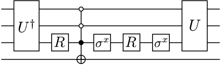
Figure A.1. A circuit that implements the controlled unitary $U_{\Pi}$ from equation (A.1) for a projector of the form (A.3). Here the controlled operation applies $\sigma^{x}$ to the fourth qubit if the first three qubits are in the state $|001\rangle$. The single qubit unitary $R$ is given by (A.4).

Our algorithm is based on the circuit in Figure A.1 which implements $U_{\Pi}$. In the Figure, the four-qubit controlled unitary is

$$|001\rangle\langle 001|\otimes\sigma^{x}+\left(\mathbb{I}-|001\rangle\langle 001|\right)\otimes\mathbb{I}$$

and

$$R=\frac{1}{\sqrt{3}}\left(\begin{array}[]{cc}\sqrt{2}&-1\\ 1&\sqrt{2}\end{array}\right).$$ (A.4)

Note that, with the exception of the single-qubit $R$ gates, all gates which appear in the circuit in Figure A.1 can be expressed as products of $\widehat{H},T$ and CNOT gates (their matrix elements are of the form (2.3)). To implement each of the $R$ gates, we use a heralded $m$-step procedure described below. Each $R$ gate succeeds with probability

$$1-\frac{1}{4^{m}}.$$

The overall probability that we apply the circuit in Figure A.1 is then $\left(1-\frac{1}{4^{m}}\right)^{2}$.

An $m$-step algorithm to implement $R$

Consider the following 2-qubit unitary

$$A=\frac{1}{2}\left(\begin{array}[]{rrrr}\sqrt{2}&-1&1&0\\ 1&\sqrt{2}&0&1\\ 1&0&-\sqrt{2}&-1\\ 0&1&1&-\sqrt{2}\end{array}\right).$$

Since each of its matrix elements is of the form (A.2), $A$ can be implemented exactly using the gate set $\{\widehat{H},T,\text{CNOT}\}$ using one ancilla initialized in the $|0\rangle$ state [10]. That is to say, the results of reference [10] can be used to obtain a sequence of $\widehat{H}$, $T$ and CNOT gates implementing a 3-qubit unitary $\tilde{U}$ such that

$$\tilde{U}|0\rangle|\psi\rangle=|0\rangle\left(A|\psi\rangle\right)$$

for all $2$-qubit states $|\psi\rangle$. Let $|\phi\rangle$ be a one-qubit state that we wish to apply $R$ to. The $m$-step algorithm consists of applying the following procedure until either a) the algorithm terminates or b) step 2 has been repeated $m$ times. In case a) the algorithm succeeds and in case b) it fails.

1. Apply $\tilde{U}$ to the state

   $$|00\rangle|\phi\rangle$$ (A.5)

   to get

   $$\tilde{U}|00\rangle|\phi\rangle=|0\rangle\left(A|0\rangle|\phi\rangle\right).$$

2. Measure the second qubit in the computational basis to obtain an outcome $z\in\{0,1\}$. Looking at the top left $2\times 2$ submatrix of $A$ we see that with probability

   $$p=\left\|\left(|0\rangle\langle 0|\otimes\mathbb{I}\right)A|0\rangle|\phi\rangle\right\|^{2}=\frac{3}{4}$$

   we get the outcome $z=0$. In this case the post-measurement state is

   $$|00\rangle R|\phi\rangle.$$

   In this case we are done–the unitary $R$ has been applied to the state $|\phi\rangle$. On the other hand, if we get the outcome $z=1$ then the post-measurement state is

   $$|01\rangle|\phi\rangle.$$

   We then discard the two ancillas, adjoin two new ones in the state $|0\rangle$ and start over from step 1.

The algorithm fails if in each of the $m$ repetitions of step 2 we measure $z=1$. This occurs with probability $\frac{1}{4^{m}}$.

Appendix B Supplementary Figures

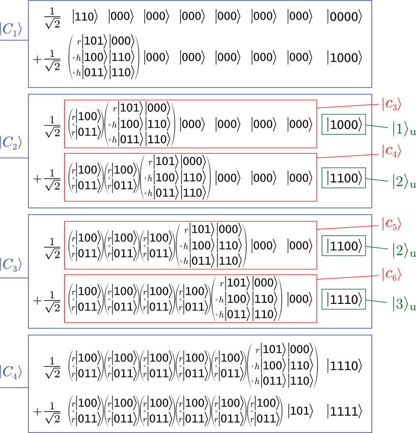
Figure B.1. The clock states $|C_{1}\rangle,|C_{2}\rangle,|C_{3}\rangle,|C_{4}\rangle$ for $N=4$, expanded in the computational basis. These states are defined through equation (3.35). We use the shorthand $r=1/\sqrt{2}$ and $h=1/2$.

Figure B.2. The terms $h_{45}(B_{b})\otimes\mathbb{I}$ and $h_{45}(\sigma^{z}_{b})$ from $H_{\text{horizontal}}$ (4.13) and $H_{\text{vertical}}$ (4.14) couple the states $|\mathcal{R}_{0}\rangle,|\mathcal{G}_{0}\rangle,|\mathcal{Y}_{0}\rangle,|\mathcal{B}_{0}\rangle$ or $|\mathcal{R}_{1}\rangle,|\mathcal{G}_{1}\rangle,|\mathcal{Y}_{1}\rangle,|\mathcal{B}_{1}\rangle$ depending on the state of the control qubit. a) When the control qubit is $|0\rangle$, the state $|0\rangle|y\rangle|\mathcal{R}_{0}\rangle$ is coupled to $|0\rangle B|y\rangle|\mathcal{G}_{0}\rangle$, which is coupled to $|0\rangle\sigma^{z}B|y\rangle|\mathcal{B}_{0}\rangle$ which is coupled to $|0\rangle B^{\dagger}\sigma^{z}B|y\rangle|\mathcal{Y}_{0}\rangle$. b) When the control qubit is $|1\rangle$, the state $|1\rangle|y\rangle|\mathcal{R}_{1}\rangle$ is coupled $|1\rangle|y\rangle\sigma^{z}|\mathcal{G}_{1}\rangle$ which is coupled to $|1\rangle B\sigma^{z}|y\rangle|\mathcal{B}_{1}\rangle$ which is coupled to $|1\rangle|y\rangle\sigma^{z}B\sigma^{z}|\mathcal{Y}_{1}\rangle$.

Appendix C Proof of Lemma 3

In this Section we prove Lemma 3. We build up the Hamiltonian

$$\mathbb{I}\otimes H_{\text{diag}}^{(M)}+\sum_{j=0}^{M-1}H_{V}^{j}+\sum_{j=0}^{M-1}H_{U}^{j}$$

a few terms at a time, lower-bounding its smallest nonzero eigenvalue at every step. The main technical tools we use are three Corollaries of Kitaev’s geometric Lemma [14] which we prove below. In this Section we will make use of, and refer repeatedly to, the details of the clock construction from Section 3.3.

C.1. Notation and spectral bounds

Let us start by establishing some notation. Recall that, if $H$ is positive semidefinite and not identically zero, we write

$$\gamma(H)$$

for its smallest nonzero eigenvalue. If $H$ is a Hamitonian acting on a Hilbert space $\mathcal{H}$ and $S$ is a subspace of $\mathcal{H}$, write

$$H|_{S}$$

for the restriction of $H$ to states in $S$ (it can be written as a $\text{dim}(S)\times\text{dim}(S)$ matrix). In this paper all Hilbert spaces and operators are finite-dimensional.

The following Corollary is a variant of Lemma 2 which (unlike the Lemma) can be used when $H$ has a nonempty nullspace.

Corollary 1.

Let $H=H_{A}+H_{B}$ where $H_{A}\geq 0$ and $H_{B}\geq 0$ each have nonempty nullspaces. Let $\Gamma$ be the subspace of states in the nullspace of $H_{A}$ that are orthogonal to the nullspace of $H$, and let $\Pi_{B}$ be the projector onto the nullspace of $H_{B}$. Then

$$\gamma\left(H\right)\geq\min\{\gamma(H_{A}),\gamma(H_{B})\}\cdot\left(1-\sqrt{d}\right)$$

where

$$d=\left\|\Pi_{B}|_{\Gamma}\right\|=\max_{|v\rangle\in\Gamma\,:\,\langle v|v\rangle=1}\langle v|\Pi_{B}|v\rangle.$$

Proof.

Let $P$ be the projector onto the nullspace of $H$ (if it is empty, set $P=0$). Define

$$H_{A}^{\prime} =H_{A}+\gamma(H_{A})\cdot P.$$

Note that every state in the nullspace of $H$ is also in the nullspace of $H_{A}$ and so $[P,H_{A}]=0$. This implies that $\gamma(H_{A}^{\prime})=\gamma(H_{A}).$ Noting that $H^{\prime}=H_{A}^{\prime}+H_{B}$ has no zero eigenvalues, we apply Lemma 2 to get

$$\gamma(H)\geq\min\{\gamma(H_{A}),\gamma(H_{B})\}\cdot\left(1-\sqrt{c}\right),$$

where

$$c=\left\|\Pi_{B}|_{S^{\prime}}\right\|$$

and $S^{\prime}$ is the groundspace of $H_{A}^{\prime}.$ Noting that $S^{\prime}=\Gamma$ (and hence $c=d$) completes the proof. ∎

We derive two additional Corollaries by upper bounding the parameter $d$ in two different ways. Let $S$ be the nullspace of $H_{A}$, and suppose that $H_{B}|_{S}$ is not the zero matrix. Note that

$$\gamma(H_{B}|_{S})=\min_{|v\rangle\in\Gamma\,:\,\langle v|v\rangle=1}\langle v|H_{B}|v\rangle,$$

since the zero eigenspace of $H_{B}|_{S}$ is equal to the nullspace of $H$. Accordingly, for any normalized state $|v\rangle\in\Gamma$,

$$\gamma(H_{B}|_{S})\leq\langle v|H_{B}|v\rangle\leq\langle v|\left(1-\Pi_{B}\right)|v\rangle\left\|H_{B}\right\|,$$

and so

$$d\leq 1-\frac{\gamma(H_{B}|_{S})}{\left\|H_{B}\right\|}.$$

Using this bound in Corollary 1 and using the fact that $1-\sqrt{1-x}\geq\frac{x}{2}$ for $x\in[0,1]$ gives the following Corollary.

Corollary 2.

Let $H=H_{A}+H_{B}$ where $H_{A}\geq 0$ and $H_{B}\geq 0$ each have nonempty nullspaces. Write $S$ for the nullspace of $H_{A}$ and suppose $H_{B}|_{S}$ is not the zero matrix. Then

$$\gamma\left(H\right)\geq\min\{\gamma(H_{A}),\gamma(H_{B})\}\cdot\frac{\gamma(H_{B}|_{S})}{2\left\|H_{B}\right\|}.$$

We now derive a different bound on $d$. For any normalized state $|v\rangle\in\Gamma$,

$$\gamma(H_{B}|_{S})\leq\langle v|\left(1-\Pi_{B}\right)H_{B}|v\rangle\leq\left(\langle v|\left(1-\Pi_{B}\right)|v\rangle\langle v|H_{B}^{2}|v\rangle\right)^{\frac{1}{2}}$$

using the Cauchy-Schwarz inequality. Squaring both sides and rearranging, we get

$$\langle v|\Pi_{B}|v\rangle\leq 1-\frac{\gamma(H_{B}|_{S})^{2}}{\langle v|H_{B}^{2}|v\rangle}\leq 1-\frac{\gamma(H_{B}|_{S})^{2}}{F},$$

where

$$F=\max_{|v\rangle\in S\,:\,\langle v|v\rangle=1}\langle v|H_{B}^{2}|v\rangle.$$ (C.1)

Since this holds for all normalized $|v\rangle\in\Gamma$, we get

$$d\leq 1-\frac{\gamma(H_{B}|_{S})^{2}}{F}.$$

Here we need $F\neq 0$, which is true whenever $H_{B}|_{S}$ is not the zero matrix. Using this bound in Corollary 1 gives

Corollary 3.

Let $H=H_{A}+H_{B}$ where $H_{A}\geq 0$ and $H_{B}\geq 0$ each have nonempty nullspaces. Write $S$ for the nullspace of $H_{A}$ and suppose $H_{B}|_{S}$ is not the zero matrix. Then

$$\gamma\left(H\right)\geq\min\{\gamma(H_{A}),\gamma(H_{B})\}\cdot\frac{\gamma(H_{B}|_{S})^{2}}{2F},$$

with $F$ defined in (C.1).

C.2. Applying the spectral bounds

We begin by proving a lower bound on the smallest nonzero eigenvalue of the Hamiltonian $H_{\text{triplet}}^{(2N)}$ from (3.10).

Lemma 4.

$$\gamma\left(H_{\textnormal{triplet}}^{(2N)}\right)\geq\frac{1}{48}.$$

Proof.

Recall that

$$H_{\text{triplet}}^{(2N)}=H_{1}+H_{2}+H_{3}$$

with $H_{1}$, $H_{2}$ and $H_{3}$ given in (3.11), (3.12), (3.13). We first show that $\gamma\left(H_{1}+H_{2}\right)$ is lower bounded by a constant. Let

$$H_{a} =\left(H_{1}+H_{2}\right)-\sum_{i=0}^{2N-2}|\theta^{-}\rangle\langle\theta^{-}|_{3i+1,3i+2,3i+3},\qquad H_{b}=\sum_{i=0}^{2N-2}|\theta^{-}\rangle\langle\theta^{-}|_{3i+1,3i+2,3i+3}$$

and note (by looking at equations (3.11), (3.12)) that $H_{a}$ is diagonal in the computational basis and is a sum of projectors. Because of this, its eigenvalues are nonnegative integers and so $\gamma\left(H_{a}\right)\geq 1.$ We now construct a convenient basis for the ground state subspace of $H_{a}.$ Recall that the groundspace of $H_{1}+H_{2}$ is spanned by states $\{|\widehat{i}\rangle\}$ and $\{|\tilde{k}\rangle\}$ from equations (3.15)-(3.16) and (3.17). We can associate a set of ground states of $H_{a}$ with each of these states. For example, look at

$$|\widehat{3}\rangle=|\theta^{+}\rangle|110\rangle|000\rangle\dots|000\rangle.$$

Note that $|\widehat{3}\rangle$ is a zero energy ground state of $H_{a}$, but so is

$$|\theta^{-}\rangle|110\rangle|000\rangle\dots|000\rangle.$$

Similarly, for each of the states $|\widehat{i}\rangle$ for $i\in\{1,\dots,4N-2\}$, we can construct additional zero energy ground states of $H_{a}$ by replacing any subset of the $|\theta^{+}\rangle$ states which appear in the tensor product by $|\theta^{-}\rangle$ states. Likewise, we obtain $2^{k}$ groundstates of $H_{a}$ from each state $|\tilde{k}\rangle$ for $k\in\{1,\dots,2N-2\}$ by making such replacements. Taking all of the states constructed in this way, we get a spanning set of ground states of $H_{a}.$ This basis for the groundspace of $H_{a}$ is convenient because every basis state is also an eigenstate of $H_{b}$ with an integer eigenvalue. This shows that the projector $\Pi_{a}$ onto the groundspace of $H_{a}$ commutes with $H_{b}$ and hence also with $H_{a}+H_{b}.$ Any eigenstate $|w\rangle$ of $H_{a}+H_{b}$ satisfying $\Pi_{a}|w\rangle=|w\rangle$ has an integer eigenvalue as discussed above. On the other hand, an eigenstate $|w^{\prime}\rangle$ with $\Pi_{a}|w^{\prime}\rangle=0$ has energy at least $\gamma(H_{a})=1$ since $H_{b}\geq 0.$ Therefore,

$$\gamma(H_{1}+H_{2})=\gamma(H_{a}+H_{b})\geq 1.$$ (C.2)

We now use Corollary 3 with $H_{A}=H_{1}+H_{2}$ and $H_{B}=H_{3}$ to bound the smallest nonzero eigenvalue of $H_{\text{triplet}}^{(2N)}$. First, note that $H_{3}$ is a sum of commuting projectors and therefore $\gamma(H_{3})=1$. Looking at (3.18), and writing $S$ for the groundspace of $H_{1}+H_{2}$, we see that $\gamma\left(H_{3}|_{S}\right)=\frac{1}{6}.$ Let us now look at the second power of $H_{3}$:

$$H_{3}^{2} = H_{3}+\sum_{i\neq j}|\gamma\rangle\langle\gamma|_{3i+3,3i+4,3i+5}\otimes|\gamma\rangle\langle\gamma|_{3j+3,3j+4,3j+5},$$

noting that every state in the groundspace of $H_{1}+H_{2}$ is annihilated by the second term in the above expression (one can easily verify this fact for each of the states $|\hat{i}\rangle$ and $|\tilde{k}\rangle$ defined in equations (3.15)-(3.16) and (3.17)). This implies that for all $|v\rangle\in S$,

$$\langle v|H_{3}^{2}|v\rangle=\langle v|H_{3}|v\rangle,$$

and hence

$$F=\max_{|v\rangle\in S}\langle v|H_{3}^{2}|v\rangle=\max_{|v\rangle\in S}\langle v|H_{3}|v\rangle=\left\|H_{B}|_{S}\right\|=\frac{2}{3},$$

where we used (3.18) to compute $\left\|H_{B}|_{S}\right\|$. Now applying Corollary 3 and using (C.2) we get

$$\gamma\left(H_{\text{triplet}}^{(2N)}\right) \geq\frac{1}{2}\cdot\frac{1}{36}\cdot\frac{3}{2}\cdot 1=\frac{1}{48}.$$ (C.3)

∎

Next, we prove a lower bound on the smallest nonzero eigenvalue of $H_{\text{clock}}^{(N)}$ from (3.28).

Lemma 5.

$$\gamma(H_{\text{{clock}}}^{(N)})\geq\frac{1}{2048}.$$

Proof.

We first bound

$$\gamma\left(H_{\text{triplet}}^{(2N)}\otimes\mathbb{I}+\mathbb{I}\otimes H_{\text{unary}}^{(N)}+H_{\text{sync}}\right),$$

where $H_{\text{unary}}^{(N)}$ and $H_{\text{sync}}$ are defined in equations (3.29) and (3.31). We will use Corollary 3 with

$$H_{A}=H_{\text{triplet}}^{(2N)}\otimes\mathbb{I}+\mathbb{I}\otimes H_{\text{unary}}^{(N)},\qquad H_{B}=H_{\text{sync}}.$$

Note that the two terms in $H_{A}$ act on different registers and therefore commute. The second term has nonnegative integer eigenvalues so

$$\gamma(H_{A})\geq\gamma(H_{\text{triplet}}^{(2N)}\otimes\mathbb{I})\geq\frac{1}{48}$$

by Lemma 4. $H_{B}$ is a sum of commuting projectors and therefore satisfies $\gamma(H_{B})=1.$ The zero energy groundspace $S$ of $H_{A}$ is spanned by states

$$|s_{ij}\rangle=|c_{j}\rangle|\underbrace{1\cdots 1}_{i}\underbrace{0\cdots 0}_{N-i}\rangle$$ (C.4)

for $i=0,\dots,N$ and $j=1,\dots 2N$, where $\{|c_{j}\rangle\}$ are the ground states of $H_{\text{triplet}}^{(2N)}$ given in (3.19)-(3.21). Using equations (3.23) and (3.24), we see that $H_{B}|_{S}$ is diagonal in the basis (C.4), with $\gamma(H_{B}|_{S})=\frac{1}{2}$. Now consider $H_{B}^{2}.$ Noting that

$$q_{j}q_{k}|c_{m}\rangle=0\quad\text{whenever}\;j\neq k,$$

and $q_{j}^{2}=q_{j}$, we get

$$H_{B}^{2}|s_{ij}\rangle=\left(q_{1}\otimes|1\rangle\langle 1|_{1}+\sum_{j=2}^{2N-1}q_{j}\otimes\left(|0\rangle\langle 0|_{\left\lfloor\frac{j}{2}\right\rfloor}+|1\rangle\langle 1|_{\left\lfloor\frac{j}{2}\right\rfloor+1}\right)^{2}+q_{2N}\otimes|0\rangle\langle 0|_{N}\right)|s_{ij}\rangle.$$

Thus $H_{B}^{2}|_{S}$ is diagonal in the basis (C.4) and we can evaluate its diagonal matrix elements using the above expression. The largest such matrix element is

$$\left\|H_{B}^{2}|_{S}\right\|=1.$$

Applying Corollary 3 with $F=1$ gives

$$\gamma\left(H_{\text{triplet}}^{(2N)}\otimes\mathbb{I}+\mathbb{I}\otimes H_{\text{unary}}^{(N)}+H_{\text{sync}}\right)\geq\frac{1}{2}\cdot\frac{1}{48}\cdot\frac{1}{4}=\frac{1}{384}.$$

As the final step, we apply Corollary 3 again, now with

$$H_{A}=H_{\text{triplet}}^{(2N)}\otimes\mathbb{I}+\mathbb{I}\otimes H_{\text{unary}}^{(N)}+H_{\text{sync}},\qquad H_{B}=\sum_{i=1}^{N}g_{2i-1,2i}(\sigma_{i}^{x}),$$

so that $H_{A}+H_{B}=H_{\text{clock}}^{(N)}.$ Recall the basis for the groundspace of $H_{A}$ given by the states $|e_{j}\rangle$ from (3.32). The restriction of $H_{B}$ to the subspace $S$ spanned by these states is given in (3.33). Looking at this expression and making use of the fact that $\beta_{j}\geq\frac{1}{4}$ for all $j$, we see that $\gamma\left(H_{B}|_{S}\right)\geq\frac{1}{2}$. Looking at (3.25) we see that the summands in $H_{B}$ are mutually commuting projectors. Since it is also the case that $g_{2i-1,2i}(\sigma_{i}^{x})|e_{k}\rangle=0$ whenever $k\notin\{2i-1,2i\}$, we see that

$$g_{2j-1,2j}(\sigma_{j}^{x})g_{2i-1,2i}(\sigma_{i}^{x})|e_{k}\rangle=\delta_{ij}g_{2i-1,2i}(\sigma_{i}^{x})|e_{k}\rangle,$$

and hence

$$H_{B}^{2}|_{S}=H_{B}|_{S}.$$

This means

$$F=\left\|H_{B}^{2}|_{S}\right\|=\left\|H_{B}|_{S}\right\|\leq\frac{2}{3},$$

using (3.33) and the fact that $\beta_{2j-1}\leq\frac{1}{3}$. Now applying Corollary 3 we get

$$\gamma\left(H_{\text{clock}}^{(N)}\right)\geq\frac{1}{2}\cdot\frac{1}{384}\cdot\frac{1}{4}\cdot\frac{3}{2}=\frac{1}{2048}.$$

∎

Now we are ready to prove a bound on the smallest nonzero eigenvalue of $H_{\text{diag}}^{(M)}$ from (5.3). Recall that this Hamiltonian acts on the Hilbert space of two clock registers, and its ground states are represented in Figure 5.1.

Lemma 6.

$$\gamma\left(H_{\textnormal{diag}}^{(M)}\right)=\Omega\left(\frac{1}{M}\right).$$

Proof.

Looking at equations (5.3) and (4.2), write

$$H_{\text{diag}}^{(M)}=H_{\alpha}+H_{\beta}+H_{\gamma},$$

where

$$H_{\alpha} =H_{\text{\text{clock}}}^{(9M+3)}\otimes\mathbb{I}+\mathbb{I}\otimes H_{\text{clock}}^{(9M+3)},$$

$$H_{\beta} =C_{\leq\left(9M+1\right)}\otimes C_{\geq\left(9M+3\right)}+\sum_{k=0}^{M-1}\left(C_{\leq\left(9k+1\right)}\otimes C_{\geq\left(9k+3\right)}+C_{\leq\left(9k+4\right)}\otimes C_{\geq\left(9k+6\right)}\right)$$

$$+C_{\geq\left(9M+3\right)}\otimes C_{\leq\left(9M+1\right)}+\sum_{k=0}^{M-1}\left(C_{\geq\left(9k+3\right)}\otimes C_{\leq\left(9k+1\right)}+C_{\geq\left(9k+6\right)}\otimes C_{\leq\left(9k+4\right)}\right),$$

$$H_{\gamma} =\sum_{k=0}^{M-1}\left(h_{9k+1,9k+2}\otimes C_{\leq(9k+2)}+h_{(9k+2),(9k+3)}\otimes C_{\geq(9k+2)}\right)$$

$$+\sum_{k=0}^{M-1}\left(C_{\leq(9k+2)}\otimes h_{9k+1,9k+2}+C_{\geq(9k+2)}\otimes h_{(9k+2),(9k+3)}\right)$$

$$+\sum_{k=0}^{M-1}\left(h_{9k+4,9k+5}\otimes C_{\leq(9k+5)}+h_{(9k+5),(9k+6)}\otimes C_{\geq(9k+5)}\right)$$

$$+\sum_{k=0}^{M-1}\left(C_{\leq(9k+5)}\otimes h_{9k+4,9k+5}+C_{\geq(9k+5)}\otimes h_{(9k+5),(9k+6)}\right)$$

$$+h_{9M+1,9M+2}\otimes C_{\leq(9M+2)}+h_{(9M+2),(9M+3)}\otimes C_{\geq(9M+2)}$$

$$+C_{\leq(9M+2)}\otimes h_{9M+1,9M+2}+C_{\geq(9M+2)}\otimes h_{(9M+2),(9M+3)}.$$

Recall that the ground state subspace $S_{\alpha}$ of $H_{\alpha}$ is spanned by the states

$$\{|C_{i}\rangle|C_{j}\rangle\,:\,(i,j)\in[9M+3]\otimes[9M+3]\}.$$ (C.5)

$H_{\beta}$ satisfies $\gamma\left(H_{\beta}\right)\geq 1$ since it is a sum of commuting projectors. Applying Corollary 1 and using the result of Lemma 5 which bounds $\gamma\left(H_{\alpha}\right)$, we get

$$\gamma\left(H_{\alpha}+H_{\beta}\right) \geq \frac{1}{2048}\cdot\left(1-\sqrt{d}\right),$$ (C.6)

$$d = \left\|\Pi_{\beta}|_{\Gamma}\right\|,$$

where $\Pi_{\beta}$ is the projector onto the groundspace of $H_{\beta}$, and $\Gamma$ is the subspace of groundstates of $H_{\alpha}$ that are orthogonal to the groundspace of $H_{\alpha}+H_{\beta}.$ Looking at the form of $H_{\beta}$ we see that a spanning set of basis vectors for the groundspace of $H_{\alpha}+H_{\beta}$ is given by a subset of the basis vectors (C.5). The set $\Gamma$ is the complement of this subset, and in particular can be written as

$$\Gamma = \text{span}\{|C_{i}\rangle|C_{j}\rangle:\left(i,j\right)\in P\}$$ (C.7)

for some set $P\subset[9M+3]\otimes[9M+3]$ (we will not need an explicit expression for $P$).

We now consider $\Pi_{\beta}|_{\Gamma}$ in the basis (C.7) and bound the norm of the resulting matrix. Recall from (3.36) and (3.37) that the operators $C_{\leq i}$ and $C_{\geq i}$ act only on the last $9M+3$ qubits of the clock register, are mutually commuting, and are diagonal in the computational basis for all $i\in[9M+3]$. This implies that $\Pi_{\beta}$ has the form

$$\Pi_{\beta}=\sum_{(z_{1},z_{2})\in\mathcal{A}}\mathbb{I}\otimes\left(|z_{1}\rangle\langle z_{1}|\right)\otimes\mathbb{I}\otimes\left(|z_{2}\rangle\langle z_{2}|\right),$$ (C.8)

where the two identity operators act on the first $6(9M+3)-3$ qubits of the two clock registers and where $\mathcal{A\subseteq}\{0,1\}^{9M+3}\otimes\{0,1\}^{9M+3}$ is a set of pairs of $(9M+3)$-bit strings (we will not require an explicit expression for $\mathcal{A}$).

Now look at the expression for the states $|C_{i}\rangle$ from equation (3.35) with $N=9M+3$ (or inspect Figure B.1) and note that

$$\langle C_{i}|\left(\mathbb{I}\otimes|z\rangle\langle z|\right)|C_{j}\rangle=0\;\text{ whenever }i\neq j,$$

where the tensor product separates the first $6N-3$ qubits from the last $N$ and where $z$ is any $N$-bit string. Using this fact and (C.8) we get

$$\langle C_{j_{2}}|\langle C_{i_{2}}|\Pi_{\beta}|C_{i_{1}}\rangle|C_{j_{1}}\rangle=0\;\text{ whenever (}i_{1},j_{1})\neq(i_{2},j_{2}).$$

We evaluate the diagonal matrix elements of $\Pi_{\beta}$ using (3.35):

$$\langle C_{j}|\langle C_{i}|\Pi_{\beta}|C_{i}\rangle|C_{j}\rangle=\frac{1}{4}\left(\delta_{(u(i-1),u(j-1))\in\mathcal{A}}+\delta_{(u(i),u(j-1))\in\mathcal{A}}+\delta_{(u(i-1),u(j))\in\mathcal{A}}+\delta_{(u(i-1),u(j-1))\in\mathcal{A}}\right),$$

where $u(i)$ is the unary representation of $i$ with $N$ bits (the bit string with $i$ ones followed by $N-i$ zeros), and $\delta_{(x,y)\in\mathcal{A}}$ is equal to one if $(x,y)\in\mathcal{A}$ and zero otherwise. Since $\Pi_{\beta}|_{\Gamma}$ is diagonal in this basis we have

$$\left\|\Pi_{\beta}|_{\Gamma}\right\| =\max_{(i,j)\in P}\langle C_{j}|\langle C_{i}|\Pi_{\beta}|C_{i}\rangle|C_{j}\rangle$$

$$=\max_{(i,j)\in P}\frac{1}{4}\left(\delta_{(u(i-1),u(j-1))\in\mathcal{A}}+\delta_{(u(i),u(j-1))\in\mathcal{A}}+\delta_{(u(i-1),u(j))\in\mathcal{A}}+\delta_{(u(i-1),u(j-1))\in\mathcal{A}}\right).$$

We know that $\left\|\Pi_{\beta}|_{\Gamma}\right\|$ is not equal to $1$ since the space $\Gamma$ does not contain any states which have zero energy for $H_{\beta}$ (by definition). Looking at the above expression for this quantity we see that this implies

$$\left\|\Pi_{\beta}|_{\Gamma}\right\|\leq\frac{3}{4}.$$

Now using this bound in (C.6) we get

$$\gamma\left(H_{\alpha}+H_{\beta}\right) = \Omega(1).$$

For the final step in the proof of Lemma 6, we use Corollary 2 with $H_{A}=H_{\alpha}+H_{\beta}$ and $H_{B}=H_{\gamma}.$ As discussed above, the ground space of $H_{A}$ is spanned by the states $|C_{i}\rangle|C_{j}\rangle$ with $(i,j)\notin P$. $H_{\gamma}$ is block-diagonal in this basis, with a block for each connected component of the graph in Figure 5.1. From this Figure we also see that blocks have maximum size equal to 7. Within each block there is a zero energy state given by the uniform superposition over states $|C_{i}\rangle|C_{j}\rangle$ where $(i,j)$ are in the associated connected component. There are also higher energy states. The lowest nonzero eigenvalue of $H_{\gamma}$ within the subspace spanned by ground states of $H_{\alpha}+H_{\beta}$ is equal to the smallest nonzero eigenvalue for one of these constant-size blocks, which is a constant independent of $M$. The norm of $H_{B}$ is upper bounded as $\left\|H_{B}\right\|=\mathcal{O}(M)$ since it is a sum of $O(M)$ projectors. Furthermore, looking at equations (3.36), (3.37) and (3.39), we see that

$$\{C_{\leq j}\},\qquad\{C_{\geq k}\},\qquad\text{and}\qquad\{h_{i,i+1}\}$$

are mutually commuting. Thus, $H_{B}$ is a sum of commuting projectors which implies that its eigenvalues are integers, and in particular $\gamma(H_{B})\geq 1$. Now applying Corollary 2 we get

$$\gamma\left(H_{\alpha}+H_{\beta}+H_{\gamma}\right)=\Omega\left(\frac{1}{M}\right),$$

which completes the proof. ∎

The next Lemma bounds the smallest nonzero eigenvalue of $\sum_{j=0}^{M-1}H_{U}^{j}$ where $H_{U}^{j}$ is defined in (5.6). The role of this Hamiltonian is to check the application of single-qubit gates $U^{j}$ within the ground state subspace of $H_{\text{diag}}^{M}$.

Lemma 7.

$$\gamma\left(\sum_{j=0}^{M-1}H_{U}^{j}\right)=\Omega(1).$$

Proof.

Recall that the operator

$$\sum_{j=0}^{M-1}H_{U}^{j}=\sum_{j=0}^{M-1}\left(h_{9j+3,9j+4}(U^{j})\otimes\mathbb{I}+\mathbb{I}\otimes\mathbb{I}\otimes h_{9j+3,9j+4}\right)$$ (C.9)

acts on a Hilbert space with an $(n+n_{a})$-qubit computational register and two clock registers

$$\left(\mathbb{C}^{2}\right)^{(n+n_{a})}\otimes\left(\mathbb{C}^{2}\right)^{7N-3}\otimes\left(\mathbb{C}^{2}\right)^{7N-3},$$

where $N=9M+3$ is the number of states for each clock. Each $U^{j}$ is either the Hadamard gate, the $T$ gate, or the identity gate acting on one of the qubits of the computational register. In (C.9), $h_{9j+3,9j+4}(U^{j})$ acts nontrivially on a single qubit of the computational register as well as qubits $6(9j+3)-1$ and $6(9j+3)$ of the first clock register (to see this, look at (3.39)).

Define operators

$$P_{i,i+1}=|01\rangle\langle 01|_{6i-1,6i}+|10\rangle\langle 10|_{6i-1,6i}$$ (C.10)

for $i=1,\dots,N-1$ which act on a single clock register. Note that we can simultaneously diagonalize (C.9) along with

$$\{\mathbb{I}\otimes P_{9j+3,9j+4}\otimes\mathbb{I}\}\quad \{\mathbb{I}\otimes\mathbb{I}\otimes h_{9j+3,9j+4}\}$$ and (C.11)

for $j=0,\dots,M-1$, since all of these operators are mutually commuting. We choose to work in a basis of simultaneous eigenvectors for these operators.

Any eigenstate $|\psi\rangle$ of (C.9), which is also a zero eigenvector of

$$\mathbb{I}\otimes P_{9j+3,9j+4}\otimes\mathbb{I},$$ (C.12)

satisfies

$$\left(h_{9j+3,9j+4}(U^{j})\otimes\mathbb{I}\right)|\psi\rangle=0.$$ (C.13)

Likewise, there are eigenstates $|\psi^{\prime}\rangle$ of (C.9) which satisfy

$$\left(\mathbb{I}\otimes\mathbb{I}\otimes h_{9j+3,9j+4}\right)|\psi^{\prime}\rangle=0.$$ (C.14)

We are working in a basis where each eigenstate of (C.9) has a set of simultaneous eigenvalues for the projectors from (C.11). An eigenstate $|\kappa\rangle$ in this basis has eigenvalue $0$ or $1$ for each of these projectors. Let us fix $|\kappa\rangle$ and consider the projectors which have eigenvalue zero. Looking at equations (C.13) and (C.14) we see that for each such projector there is a corresponding term in (C.9) that annihilates $|\kappa\rangle.$ Let us now focus our attention on the other terms in (C.9). Specifically, for a given eigenstate $|\kappa\rangle$ of (C.9), consider the terms

$$h_{9j+3,9j+4}(U^{j})\otimes\mathbb{I},$$

where $\left(\mathbb{I}\otimes P_{9j+3,9j+4}\otimes\mathbb{I}\right)|\kappa\rangle=|\kappa\rangle$, and the terms

$$\mathbb{I}\otimes\mathbb{I}\otimes h_{9k+3,9k+4},$$

where $\left(\mathbb{I}\otimes\mathbb{I}\otimes h_{9k+3,9k+4}\right)|\kappa\rangle=|\kappa\rangle$. We’ll call these terms the remaining operators for the state $|\kappa\rangle$ (they remain after removing some terms in equation (C.9) which have eigenvalue zero).

We classify the eigenstates of (C.9) into two types. The first type of eigenstate is defined by the property that all of its remaining operators commute. Note that an eigenstate of (C.9) is also an eigenstate of the sum of its remaining operators. In this case the remaining operators are commuting projectors, and so each eigenvalue of (C.9) associated with such an eigenstate is a nonnegative integer.

The second type of eigenstate has at least two remaining operators which do not commute. Looking at (C.9) we see that these two operators must be

$$h_{9j+3,9j+4}(U^{j}),\qquad\text{and}\qquad h_{9k+3,9k+4}(U^{k}),$$

for some $j$ and $k$ with $[U^{j},U^{k}]\neq 0.$ Recall that both $U^{j}$ and $U^{k}$ are either Hadamard, $T$ or the identity acting on one of the qubits. The condition that $[U^{j},U^{k}]\neq 0$ means that the two gates must act on the same qubit, and that one of them is the Hadamard gate and the other is the $T$ gate. We now show that any eigenstate of this second type has eigenvalue $e$ bounded below by a positive constant. Since each term in (C.9) is a projector, we have

$$e_{\text{}}\geq\min_{|\psi\rangle\in S}\langle\psi|h_{9j+3,9j+4}(U^{j})+h_{9k+3,9k+4}(U^{k})|\psi\rangle,$$ (C.15)

where $S$ is the subspace of states satisfying

$$\left(\mathbb{I}\otimes P_{9j+3,9j+4}\otimes\mathbb{I}\right)|\psi\rangle=|\psi\rangle\quad\text{and}\quad\left(\mathbb{I}\otimes P_{9k+3,9k+4}\otimes\mathbb{I}\right)|\psi\rangle=|\psi\rangle.$$

For states $|\psi\rangle\in S$, the Hamiltonian

$$h_{9j+3,9j+4}(U^{j})+h_{9k+3,9k+4}(U^{k})$$ (C.16)

acts nontrivially within an $8$-dimensional space that is the tensor product of three 2-dimensional spaces. These are: the states of the single computational qubit on which the unitaries $U^{j}$ and $U^{k}$ act, the states $|01\rangle,|10\rangle$ on qubits $6(9j+3)-1,6(9j+3)$ of the first clock register, and the states $|01\rangle,|10\rangle$ on qubits $6(9k+3)-1,6(9k+3)$ of the first clock register (note $j\neq k$). Identifying this 8-dimensional space with the space of $3$ qubits, we can write the action of (C.16) as the Hamiltonian

$$\frac{1}{2}\left(\mathbb{I}\otimes\mathbb{I}\otimes\mathbb{I}-\widehat{H}\otimes|1\rangle\langle 0|\otimes\mathbb{I}-\widehat{H}\otimes|1\rangle\langle 0|\otimes\mathbb{I}\right)$$ (C.17)

$$+ \frac{1}{2}\left(\mathbb{I}\otimes\mathbb{I}\otimes\mathbb{I}-T^{\dagger}\otimes\mathbb{I}\otimes|1\rangle\langle 0|-T\otimes\mathbb{I}\otimes|0\rangle\langle 1|\right).$$

Here we used the fact that $U^{j}$ and $U^{k}$ are the Hadamard and $T$ gates respectively. Equation (C.15) says that $e_{\text{}}$ is lower bounded by the smallest eigenvalue of this operator, which is a positive constant equal to $0.00937\dots$.

Let us now summarize what we have shown regarding the eigenstates of (C.9). We have classified each eigenstate as either type 1 or type 2 according to the form of its remaining operators. We showed that every eigenstate of the first type has a nonnegative integer eigenvalue, and that every eigenstate of the second type has eigenvalue at least $0.00937\dots$. From this we see that

$$\gamma\left(\sum_{j=0}^{M-1}H_{U}^{j}\right)$$

is at least $0.00937\dots$, which completes the proof. ∎

We now prove a lower bound on the smallest nonzero eigenvalue of $\sum_{j=0}^{M-1}H_{V}^{j}$ where $H_{V}^{j}$ is defined in (5.7). The role of this Hamiltonian is to check each of the $M$ applications of the two-qubit gate $V$ within the ground state subspace of $H_{\text{diag}}^{M}$.

Lemma 8.

$$\gamma\left(\sum_{j=0}^{M-1}H_{V}^{j}\right)=\Omega(1).$$

Proof.

We use a similar strategy to that used in Lemma 7. First, we define a set of mutually commuting projectors which also commute with

$$\sum_{j=0}^{M-1}H_{V}^{j}=\sum_{j=0}^{M-1}\left(H_{\text{horizontal}}^{j}+H_{\text{vertical}}^{j}\right).$$ (C.18)

The specific set of projectors reflects the structure of the terms appearing in (C.18) (look at equations (5.8) and (5.9)). In particular, consider the set of projectors

$$\mathbb{I}\otimes h_{9j+6,9j+7}\otimes\mathbb{I} \mathbb{I}\otimes\mathbb{I}\otimes h_{9j+6,9j+7}$$ (C.19)

$$\mathbb{I}\otimes h_{9j+6,9j+7}\otimes C_{\geq 9j+10} \mathbb{I}\otimes C_{\geq 9j+10}\otimes h_{9j+6,9j+7}$$ (C.20)

$$\mathbb{I}\otimes h_{9j+8,9j+9}\otimes C_{\leq 9j+6} \mathbb{I}\otimes C_{\leq 9j+6}\otimes h_{9j+8,9j+9}$$ (C.21)

$$\mathbb{I}\otimes h_{9j+9,9j+10}\otimes\mathbb{I} \mathbb{I}\otimes\mathbb{I}\otimes h_{9j+9,9j+10}$$ (C.22)

$$\mathbb{I}\otimes h_{9j+9,9j+10}\otimes C_{\geq 9j+10} \mathbb{I}\otimes C_{\geq 9j+10}\otimes h_{9j+9,9j+10}$$ (C.23)

$$\mathbb{I}\otimes h_{9j+8,9j+9}\otimes C_{\geq 9j+10} \mathbb{I}\otimes C_{\geq 9j+10}\otimes h_{9j+8,9j+9}$$ (C.24)

$$\mathbb{I}\otimes P_{9j+7,9j+8}\otimes\mathbb{I} \mathbb{I}\otimes\mathbb{I}\otimes P_{9j+7,9j+8}$$ (C.25)

for $j=0,\dots,M-1$, where $P_{i,i+1}$ is defined in (C.10). Recall that the three registers separated by tensor products are the $(n+n_{a})$-qubit computational register, the first clock register and the second clock register. Using the definitions (3.39), (3.36) and (3.37) one can check that these projectors are mutually commuting and that they commute with (C.18). We can therefore simultaneously diagonalize (C.18) along with the projectors listed above. We choose to work in a basis of eigenstates of (C.18) in which all of these operators are diagonal.

For a given eigenstate $|\kappa\rangle$ of (C.18), each of the projectors in equations (C.19)-(C.25) can have eigenvalue either $0$ or $1$. We defined the projectors above in such a way that, if one of them has eigenvalue zero then one of the terms in (C.18) annihilates $|\kappa\rangle$. For example, if

$$\left(\mathbb{I}\otimes P_{7,8}\otimes\mathbb{I}\right)|\kappa\rangle=0$$

(this is the seventh projector from the top in the left column of equations (C.19)-(C.25) with $j=0$), then

$$\left(h_{7,8}(B_{b_{0}})\otimes\mathbb{I}\right)|\kappa\rangle=0$$

(this is the seventh term in (5.8) with $j=0$). In this way, each of the $7$ projectors on the left-hand (right-hand) column of equations (C.19)-(C.25) is associated with one of the $7$ terms in $H_{\text{horizontal}}^{j}$ ($H_{\text{vertical}}^{j}).$ To see this, compare equations (C.19)-(C.25) with equations (5.8) and (5.9). Now let us fix an eigenstate $|\kappa\rangle$ of (C.18), which has a specific set of eigenvalues for the projectors in equations (C.19)-(C.25). For each of the projectors (from the list (C.19)-(C.25) ) for which $|\kappa\rangle$ has eigenvalue $1$, consider the corresponding term from equations (5.8) and (5.9). We call these terms the remaining operators for $|\kappa\rangle$ and we classify eigenstates into two types based on these terms.

The first type of eigenstate has the property that all of its remaining operators commute. Any eigenvector of (C.18) of this type is an eigenvector of a sum of commuting projectors and therefore has an integer eigenvalue. Therefore, the lowest nonzero eigenvalue for this first type of eigenstate is at least $1.$

Now consider a second type of eigenstate where at least two of its remaining operators do not commute. Looking at equations (5.8) and (5.9) we see that possible pairs of noncommuting remaining operators are

(1): $|1\rangle\langle 1|_{a_{j}}\otimes\mathbb{I}\otimes h_{9j+6,9j+7}$ and $h_{9k+7,9k+8}(B_{b_{k}})$ with $a_{j}=b_{k}$ (and hence $j\neq k$), or

(2): $|0\rangle\langle 0|_{a_{j}}\otimes h_{9j+6,9j+7}\otimes\mathbb{I}$ and $h_{9k+7,9k+8}(B_{b_{k}})$ with $a_{j}=b_{k}$ (and hence $j\neq k$), or

(3): $h_{9j+7,9j+8}(B_{b_{j}})\otimes\mathbb{I}$ and $h_{9k+7,9k+8}(\sigma_{b_{k}})$ with $b_{k}=b_{j}$ (it may be that $j=k$).

We claim that any eigenstate $|\kappa\rangle$ of (C.18) of this second type has eigenvalue bounded below by a positive constant. To see this, first suppose two of the remaining operators are of the form (1). For these to be remaining operators it must be the case that $|\kappa\rangle$ is a $+1$ eigenvector of both

$$\mathbb{I}\otimes\mathbb{I}\otimes h_{9j+6,9j+7}\qquad\text{and}\qquad\mathbb{I}\otimes\mathbb{I}\otimes P_{9k+7,9k+8}.$$ (C.26)

The eigenvalue associated with this state is bounded below by the smallest eigenvalue of

$$|1\rangle\langle 1|_{a_{j}}\otimes\mathbb{I}\otimes h_{9j+6,9j+7}+h_{9k+7,9k+8}(B_{b_{k}})$$ (C.27)

within the joint $+1$ eigenspace of the two projectors (C.26). Within this space, (C.27) acts nontrivially on an 4-dimensional space that is the tensor product of two dimensional spaces: the single qubit space for qubit $a_{j}=b_{j}$ of the computational register and the space spanned by the two basis states $|01\rangle,|10\rangle$ of qubits $6(9j+7)-1$ and $6(9j+7)$ of the second clock register. Within this space (C.27) has the form (identifying the 4-dimensional space with two qubits):

$$|1\rangle\langle 1|\otimes\mathbb{I}+\frac{1}{2}\left(\mathbb{I}\otimes\mathbb{I}-B^{\dagger}\otimes|1\rangle\langle 0|-B\otimes|0\rangle\langle 1|\right),$$

which has smallest eigenvalue $\thickapprox 0.076$. Any eigenstate $|\kappa\rangle$ which has two remaining operators of the form (1) has eigenvalue bounded below by this positive constant. In cases (2) and (3) we can follow the same steps (as in case (1) above) to lower bound the eigenvalue. In case (2) we bound it by the smallest eigenvalue of the 2-qubit operator

$$|0\rangle\langle 0|\otimes\mathbb{I}+\frac{1}{2}\left(\mathbb{I}\otimes\mathbb{I}-B^{\dagger}\otimes|1\rangle\langle 0|-B\otimes|0\rangle\langle 1|\right)$$

(which is $\thickapprox 0.076$) and in case (3) we get a lower bound from the smallest eigenvalue of the $3$-qubit operator

$$\frac{1}{2}\left(\mathbb{I}\otimes\mathbb{I}\otimes\mathbb{I}-B^{\dagger}\otimes|1\rangle\langle 0|\otimes\mathbb{I}-B\otimes|0\rangle\langle 1|\otimes\mathbb{I}\right)+\frac{1}{2}\left(\mathbb{I}\otimes\mathbb{I}\otimes\mathbb{I}-\sigma^{z}\otimes\mathbb{I}\otimes|1\rangle\langle 0|-\sigma^{z}\otimes\mathbb{I}|\otimes|0\rangle\langle 1|\right)$$

(it is also $\thickapprox 0.076$).

We have thus shown that any eigenstate (of (C.18)) of the first type has a nonnegative integer eigenvalue and any eigenstate of the second type has smallest eigenvalue bounded below by a positive constant. This completes the proof. ∎

We now add the two-qubit gate terms to $\mathbb{I}\otimes H_{\text{diag}}^{(M)}$ and we lower bound the smallest nonzero eigenvalue of the resulting Hamiltonian.

Lemma 9.

$$\gamma\left(\mathbb{I}\otimes H_{\text{diag}}^{(M)}+\sum_{j=0}^{M-1}H_{V}^{j}\right)=\Omega\left(\frac{1}{M^{2}}\right).$$

Proof.

We apply Corollary 2 with

$$H_{A} = \mathbb{I}\otimes H_{\text{diag}}^{(M)},$$

$$H_{B} = \sum_{j=0}^{M-1}H_{V}^{j}.$$

However, we first need to understand the action of $H_{B}$ on the groundspace $S$ of $H_{A}$. We showed in Section 5.1 that $H_{B}|_{S}$, written in the unnormalized basis (5.11), is block diagonal. Of course, the matrix has the same block diagonal structure when written in a normalized basis. Furthermore, each nonzero block is identical, equal to a specific $100\times 100$ matrix (independent of $M$ or the number of qubits). The smallest nonzero eigenvalue of $\gamma(H_{B}|_{S})$ is therefore constant, equal to the smallest nonzero eigenvalue of this matrix. Plugging this into Corollary 2 and using the facts that $\left\|H_{B}\right\|=\mathcal{O}(M)$, $\gamma(H_{A})=\Omega\left(\frac{1}{M}\right)$ (from Lemma 6) and $\gamma(H_{B})=\Omega(1)$ (from Lemma 8) we get

$$\gamma\left(\mathbb{I}\otimes H_{\text{diag}}^{(M)}+\sum_{j=0}^{M-1}H_{V}^{j}\right)=\Omega\left(\frac{1}{M^{2}}\right).$$

∎

C.3. Proof of Lemma 3

We are now ready to finish the proof of Lemma 3, the main result of this Appendix. We add in the single-qubit gate terms $H_{U}^{j}$ and we use the bound from Lemma 7. We prove

$$\gamma\left(\mathbb{I}\otimes H_{\text{diag}}^{(M)}+\sum_{j=0}^{M-1}H_{V}^{j}+\sum_{j=0}^{M-1}H_{U}^{j}\right)=\Omega\left(\frac{1}{M^{5}}\right).$$

Proof.

Let

$$H_{A} =\mathbb{I}\otimes H_{\text{diag}}^{(M)}+\sum_{j=0}^{M-1}H_{V}^{j},$$

$$H_{B} =\sum_{j}H_{U}^{j},$$

and consider the action of $H_{B}$ on the groundspace $S$ of $H_{A}.$ Recall the (unnormalized) basis for the groundspace of $H_{A}$ given in equations (5.19) and (5.21), where $|\phi\rangle$ ranges over a complete orthonormal basis $\Lambda$ of the $n+n_{a}$-qubit computational register. As noted in Section 5, $H_{B}|_{S}$ is block diagonal in this basis with $2^{n+n_{a}}$ blocks because $H_{B}$ only connects states associated with the same $|\phi\rangle\in\Lambda.$ Furthermore, each block of $H_{B}|_{S}$ in this unnormalized basis is equal to $\frac{1}{4}L$ where $L$ is the Laplacian of the graph in Figure 5.2. We can write each block of $H_{B}|_{S}$ in an orthonormal basis as

$$\frac{1}{4}DLD,$$

where

$$D=\text{diag}\left(\frac{1}{\sqrt{7}},\frac{1}{\sqrt{4}},\frac{1}{\sqrt{4}},\frac{1}{\sqrt{43}},\frac{1}{\sqrt{4}},\frac{1}{\sqrt{4}},\frac{1}{\sqrt{43}},\dots,\frac{1}{\sqrt{4}},\frac{1}{\sqrt{4}},\frac{1}{\sqrt{43}}\right)$$

takes care of the normalizations (as per (5.22)). Thus, $\gamma(H_{B}|_{S})$ is equal to $\gamma\left(\frac{1}{4}DLD\right)$, which we now bound. First, note that

$$\gamma(L)=\Omega\left(\frac{1}{M^{2}}\right),$$

which follows from known bounds on the eigenvalue gap of a Laplacian matrix (for example from Theorem 4.2 of reference [19]). To finish the proof we relate $\gamma(L)$ to $\gamma\left(\frac{1}{4}DLD\right).$ Let $|w_{0}\rangle$ be the normalized all ones vector, the unique zero energy vector for $L$. Then, up to normalization, $\frac{1}{D}|w_{0}\rangle$ is the unique zero energy state for $\frac{1}{4}DLD$, and for some normalized vector $|v\rangle$ satisfying

$$\langle w_{0}|D^{-1}|v\rangle=0,$$ (C.28)

we have

$$\gamma\left(\frac{1}{4}DLD\right) =\frac{1}{4}\langle v|DLD|v\rangle$$

$$=\frac{1}{4}\frac{\langle q|L|q\rangle}{\langle q|q\rangle}\langle v|D^{2}|v\rangle$$

$$\geq\frac{1}{4}\frac{\langle q|L|q\rangle}{\langle q|q\rangle}\frac{1}{43},$$ (C.29)

where $|q\rangle=D|v\rangle$ and we used the fact that the smallest eigenvalue of $D^{2}$ is $\frac{1}{43}$. Write

$$|q\rangle=\alpha|w_{0}\rangle+\beta|w_{\perp}\rangle,$$

where $\langle w_{\perp}|w_{0}\rangle=0$ and $\langle w_{0}|w_{0}\rangle=\langle w_{\perp}|w_{\perp}\rangle=1$ and note that

$$\langle w_{0}|D^{-1}|v\rangle=\langle w_{0}|D^{-2}|q\rangle=\alpha\langle w_{0}|D^{-2}|w_{0}\rangle+\beta\langle w_{0}|D^{-2}|w_{\perp}\rangle=0$$

by (C.28) and hence

$$\left|\frac{\alpha}{\beta}\right|=\frac{\left|\langle w_{0}|D^{-2}|w_{\perp}\rangle\right|}{\langle w_{0}|D^{-2}|w_{0}\rangle}\leq\frac{43}{4},$$

where we used the facts that the smallest eigenvalue of $D^{-2}$ is $4$ and its largest eigenvalue is $43.$ Noting that

$$\frac{\langle q|L|q\rangle}{\langle q|q\rangle} =\frac{\beta^{2}}{\alpha^{2}+\beta^{2}}\langle w_{\perp}|L|w_{\perp}\rangle$$

$$\geq\frac{1}{\left(\left(\frac{43}{4}\right)^{2}+1\right)}\gamma(L)$$

$$=\Omega\left(\frac{1}{M^{2}}\right),$$

we get

$$\gamma(H_{B}|_{S})=\gamma\left(\frac{1}{4}DLD\right)=\Omega\left(\frac{1}{M^{2}}\right)$$

by plugging into (C.29). Now applying Corollary 2, using Lemmas 7 and 9 and using the bound $\left\|H_{B}\right\|=\mathcal{O}(M)$, we finally get the desired result. ∎

References

- [1] Sergey Bravyi, personal communication.
- [2] Scott Aaronson. On perfect completeness for qma. Quantum Info. Comput., 9(1):81–89, January 2009.
- [3] A. Ambainis, J. Kempe, and O. Sattath. A quantum lovász local lemma. In Proceedings of the 42nd ACM symposium on Theory of computing, pages 151–160. ACM, 2010.
- [4] S. Bravyi. Efficient algorithm for a quantum analogue of 2-SAT. eprint arXiv:quant-ph/0602108, February 2006. Published in Contemporary Mathematics Volume 536, 2011.
- [5] Sergey Bravyi, Libor Caha, Ramis Movassagh, Daniel Nagaj, and Peter W. Shor. Criticality without frustration for quantum spin-1 chains. Phys. Rev. Lett., 109:207202, Nov 2012.
- [6] Sergey Bravyi, Cristopher Moore, and Alexander Russell. Bounds on the quantum satisfiability threshold. In ICS, pages 482–489, 2010.
- [7] M. Coudron and R. Movassagh. Unfrustration Condition and Degeneracy of Qudits on Trees. ArXiv e-prints, September 2012.
- [8] Lior Eldar and Oded Regev. Quantum sat for a qutrit-cinquit pair is qma1-complete. In ICALP (1), pages 881–892, 2008.
- [9] Richard Feynman. Quantum mechanical computers. Optics News, 11:11–46, 1985.
- [10] B. Giles and P. Selinger. Exact synthesis of multi-qubit Clifford+T circuits. ArXiv e-prints, December 2012.
- [11] Zhengfeng Ji, Zhaohui Wei, and Bei Zeng. Complete characterization of the ground-space structure of two-body frustration-free hamiltonians for qubits. Phys. Rev. A, 84:042338, Oct 2011.
- [12] Stephen P. Jordan, Hirotada Kobayashi, Daniel Nagaj, and Harumichi Nishimura. Achieving perfect completeness in classical-witness quantum merlin-arthur proof systems. Quantum Info. Comput., 12(5-6):461–471, May 2012.
- [13] Julia Kempe, Alexei Kitaev, and Oded Regev. The complexity of the local hamiltonian problem. SIAM J. Comput., 35(5):1070–1097, May 2006.
- [14] A. Yu. Kitaev, A. H. Shen, and M. N. Vyalyi. Classical and Quantum Computation. American Mathematical Society, Boston, MA, USA, 2002.
- [15] Hirotada Kobayashi, François Le Gall, and Harumichi Nishimura. Stronger methods of making quantum interactive proofs perfectly complete. 4th ACM Innovations in Theoretical Computer Science conference (ITCS 2013), 2013.
- [16] C. R. Laumann, A. M. Läuchli, R. Moessner, A. Scardicchio, and S. L. Sondhi. Product, generic, and random generic quantum satisfiability. Phys. Rev. A, 81:062345, Jun 2010.
- [17] Christopher R. Laumann, R. Moessner, Antonello Scarddichio, and S. L. Sondhi. Random quantum satisfiability. Quantum Information & Computation, 10(1&2):1–15, 2010.
- [18] Chris Marriott and John Watrous. Quantum arthur—merlin games. Comput. Complex., 14(2):122–152, June 2005.
- [19] Bojan Mohar. Eigenvalues, diameter, and mean distance in graphs. Graphs and Combinatorics, 7:53–64, 1991. 10.1007/BF01789463.
- [20] R. Movassagh, E. Farhi, J. Goldstone, D. Nagaj, T. J. Osborne, and P. W. Shor. Unfrustrated qudit chains and their ground states. Physical Review A, 82(1):012318, July 2010.
- [21] D. Nagaj. Fast universal quantum computation with railroad-switch local Hamiltonians. Journal of Mathematical Physics, 51(6):062201, June 2010.
- [22] D. Nagaj and S. Mozes. New construction for a QMA complete three-local Hamiltonian. Journal of Mathematical Physics, 48(7):072104, July 2007.
- [23] Daniel Nagaj, Pawel Wocjan, and Yong Zhang. Fast amplification of qma. Quantum Information & Computation, pages 1053–1068, 2011.
- [24] T. J. Osborne. Hamiltonian complexity. Reports on Progress in Physics, 75(2):022001, February 2012.
- [25] Stathis Zachos and Martin Furer. Probabilistic quantifiers vs. distrustful adversaries. In Proc. of the seventh conference on Foundations of software technology and theoretical computer science, pages 443–455, London, UK, UK, 1987. Springer-Verlag.