Multi-Particle Spectral Properties in the Transverse Field Ising Model by Continuous Unitary Transformations

Abstract

The one-dimensional transverse field Ising model is solved by continuous unitary transformations in the high-field limit. A high accuracy is reached due to the closure of the relevant algebra of operators which we call string operators. The closure is related to the possibility to map the model by Jordan-Wigner transformation to non-interacting fermions. But it is proven without referring to this mapping. The effective model derived by the continuous unitary transformations is used to compute the contributions of one, two, and three elementary excitations to the diagonal dynamic structure factors. The three-particle contributions have so far not been addressed analytically, except close to the quantum critical point.

I Introduction

Understanding strong quantum fluctuations continues to be a formidable challenge. Where two (or more) phases compete and are separated by a continuous quantum phase transition Sachdev (2001), i.e., at zero temperature, such fluctuations are particularly strong. Generically, such a quantum phase transition is signaled by the decay of elementary excitations. Far away from the phase transition, spectroscopic probes show dominant sharp $\delta$-peaks at low energies which result from stable elementary excitations, so-called quasi-particles. But on approaching the phase transition, the spectral weight in the dominant quasi-particle peak is reduced further and further and shifted to contributions of more quasi-particle. Multi-particle spectra with considerable weight are an important signature of dominant quantum fluctuations in general. The vanishing of the single quasi-particle peaks at zero temperature is a smoking gun for a quantum phase transition in particular.

In this context, the transverse field Ising model (TFIM)Katsura (1962) is a popular generic model describing magnetic excitations and displaying a quantum phase transition between the disordered phase in the limit of dominating transverse field and the ordered phase in the limit of dominating longitudinal Ising coupling. Due to its relative simplicity, the TFIM provides a convenient test case in the development of theoretical approaches Vidal (2007); H. Y. Yang and K. P. Schmidt (2011). This is particularly true for the one dimensional case, for which fermionization by a Jordan-Wigner transformation P. Jordan and E. Wigner (1928) yields an exact solution Niemeijer (1967); Pfeuty (1970); O. Derzhko and T. Krokhmalskii (1997).

The calculation of dynamical correlations in the TFIM is an active field of research. While transverse correlations can be treated in terms of fermions O. Derzhko and T. Krokhmalskii (1997); O. Derzhko, T. Verkholyak, T. Krokhmalskii and H. Büttner (2006), longitudinal correlations require different approaches, because of their non-locality in the fermionic picture. Based on an equation of motion for the longitudinal correlations Perk (1980) there has been a series of papers investigating the scaling region around the critical point Ref. McCoy et al., 1983a, b; Müller and Shrock, 1983, 1984a, 1984b, 1985. In 2009, Perk and Au-Yang computed results for the time-dependent longitudinal correlation functions by solving the coupled differential equations and complementing them with long-time asymptotics Perk and Au-Yang (2009). But so far no momentum and frequency resolved analysis has been performed, which also applies away from the scaling regime.

Quantum magnets in the vicinity of quantum phase transitions are dominated by strong quantum fluctuations. Quantum fluctuations are strongly favored by low-dimensionality and by frustration. Theoretically, a particularly clear sign of dominant quantum fluctuations is the fractionalization of elementary excitations. For instance, conventional spin waves (magnons) split into two spinons in antiferromagnetic Heisenberg chains Faddeev and Takhtajan (1981); Nagler et al. (1991); Dender et al. (1996); Karbach et al. (1997). Before complete fractionalization occurs, the spectral weight, as observed in inelastic neutron scattering, shifts from the channel of a single elementary excitation to the channel where two and more elementary excitations are created Knetter et al. (2001); Schmidt and Uhrig (2005). Thus, also the experimental focus is directed more and more to continua formed by more than one excitation, see for instance Refs. Nagler et al., 1991; Dender et al., 1996; Notbohm et al., 2007; Christensen et al., 2007.

In view of the above considerations, the present article pursues two goals in a study of the one-dimensional (1D) TFIM. First, we show how the special algebraic structure (‘string algebra’) of the operators occurring in the 1D TFIM enables its solution by a continuous unitary transformation (CUT) in the high-field phase to very high accuracy. Upon completion of our calculations, we learned that this algebra was introduced and used before in an algebraic solution of the TFIM Jha and Valatin (1973).

This algebra paves the way to treat a larger class of models of which the Hamilton operators can be expressed by operators belonging to the string algebra, for instance $XY$ models in transverse fields. Second, we compute the three-particle contributions to the diagonal dynamic structure factors (DSF) in the CUT framework in the high-field phase. To our knowledge, this is the first time that these subdominant contributions are computed, except in the scaling region around the quantum phase transition. Thereby, interesting predictions for future experimental studies are provided.

In Sect. II, the model and known exact results are recalled. In the following section, the continuous unitary transformations (CUTs) are briefly reviewed. Sect. IV is devoted to the algebra of string operators which are subsequently employed. Sects. V and VI comprise our static and dynamic results, respectively, while the conclusions are drawn in Sect. VII.

II Model and exact results

The Hamiltonian for the transverse field Ising model (TFIM) reads

$$H_{\mathrm{TFIM}} =\frac{\Gamma}{2}\sum\limits_{i}\sigma_{i}^{z}+\frac{J}{4}\sum\limits_{i}\sigma_{i}^{x}\sigma_{i+1}^{x},$$ (1)

where the $\sigma^{\alpha}$ are the Pauli matrices and the sum $i$ runs over all lattice sites. We normalized the distance between two sites to one. The transverse field strength is given by the parameter $\Gamma$ while $J$ denotes the strength of the antiferromagnetic coupling between two adjacent sites. The antiferromagnetic exchange can be converted to a ferromagnetic exchange $J\rightarrow-J$ by a $\pi$ rotation around $S_{i}^{z}$ for every second site $i$. This translates to a shift of $\pi$ in momentum space.

The model has a quantum phase transition at $J=2\Gamma$ and it is self dual Sachdev (2001). Similar to Ref. Sachdev, 2001, we introduce the parameter $x=J/2\Gamma$. The starting point for the CUT calculations is $J=0$. Hence, an elementary excitation is given by a single spin flip. For finite $J$ the energy of these excitations becomes momentum dependent. We will refer to these excitations as quasi-particles. We expect that the perturbative ansatz breaks down once we reach the critical value $J=2\Gamma$. Hence we focus on the static and dynamic properties for $J<2\Gamma$.

The model was solved exactly by Pfeuty in 1970 Pfeuty (1970), based on the work by Lieb et al. E. Lieb, T. Schultz and D. Mattis (1961) and Niemeijer Niemeijer (1967). Pfeuty’s solution uses the Jordan-Wigner transformation P. Jordan and E. Wigner (1928) to map the Hamiltonian in Eq. (1) to a chain of free fermions which is diagonalized by a Bogoliubov transformation Bogoliubov (1947). This approach yields the exact expression for the ground state energy per site

$$\frac{E_{0}}{N\Gamma}=-\frac{1}{2\pi}\int\limits_{0}^{\pi}\omega(q)\mathrm{d}q,$$ (2)

where $\omega(q)$ denotes the dimensionless dispersion

$$\omega(q)=\sqrt{1+x^{2}-2x\cos(q)}.$$ (3)

The dispersion with dimension is given by $\Gamma\omega(q)$.

From the dispersion we can easily extract the energy gap of the lowest lying excitations

$$\frac{\Delta}{\Gamma}=\left|1-x\right|.$$ (4)

Another interesting quantity worked out by Pfeuty is the transverse magnetization

$$M_{z}=\frac{1}{N}\sum\limits_{i}\left\langle g\right|\sigma_{i}^{z}\left|g\right\rangle=\frac{1}{\pi}\int\limits_{0}^{\pi}\frac{1+x\cos(q)}{\omega(q)}\mathrm{d}q,$$ (5)

where $\left|g\right\rangle$ denotes the ground state of the TFIM. In the following sections we will compare our results with these exact expressions in order to validate the CUT approach.

Beside the static properties stated above, dynamic properties are important in order to explain experimental results. Although the TFIM is analytically integrable, the evaluation of longitudinal dynamic correlations remains a very difficult task which requires considerable numerics, see for instance Refs. Perk and Au-Yang, 2009 or Krones and Stolze, 2011. In the fermionic picture, this is due to the non-locality of the Jordan-Wigner transformation.

One important quantity in the study of spin systems is the dynamic structure factor (DSF)

$$S^{\alpha\beta}(\omega,Q) =\frac{1}{N}\int_{-\infty}^{\infty}\frac{\mathrm{d}t}{2\pi}\sum\limits_{l,l^{\prime}}e^{i\omega t}e^{-iQ(l-l^{\prime})}\langle\sigma_{l}^{\alpha}(t)\sigma_{l^{\prime}}^{\beta}\rangle,$$ (6)

where $\alpha,\beta\in\left\{x,y,z\right\}$. Here $Q$ denotes the total momentum and $\omega$ the frequency. The DSF is directly linked to the differential cross section in inelastic scattering experiments, see for instance Ref. Lovesey, 1987.

Due to the symmetry $\sigma_{i}^{x}\rightarrow-\sigma_{i}^{x}$ of $H_{\mathrm{TFIM}}$ no correlations occur for $\alpha=x,\beta=z$ and $\alpha=y,\beta=z$ and vice versa, but for $\alpha=x,\beta=y$ and for $\alpha=\beta$ the DSF may and will obtain finite values.

In the following, we focus on the diagonal part of the DSF, i.e., $\alpha=\beta$. For $\alpha=z$ exact expressions are known J. H. Taylor and G. Müller (1985); O. Derzhko and T. Krokhmalskii (1997); O. Derzhko, T. Verkholyak, T. Krokhmalskii and H. Büttner (2006), because the observable $\sigma^{z}$ remains local in the Jordan-Wigner representation of the TFIM. At zero temperature case, this expression reads

$$S^{zz}(Q,\omega) =\int\limits_{-\pi}^{\pi}\mathrm{d}k_{1}\left[1-f(Q,k_{1})\right]$$

$$\delta(\omega-\omega(k_{1}-Q/2)-\omega(k_{1}+Q/2)),$$ (7a)

with

$$f(Q,k_{1}) =\frac{\left(\Gamma+\frac{J}{2}\cos(k_{1}-Q/2)\right)\left(\Gamma+\frac{J}{2}\cos(k_{1}+Q/2)\right)}{\omega(k_{1}-Q/2)\omega(k_{1}+Q/2)}.$$ (7b)

It consists of a spectral density of scattering states of two elementary excitations with total momentum $Q$. For $\alpha=x$ and $\alpha=y$, only the one-particle contributions have been calculated by Hamer et al. in 2006 C. J. Hamer, J. Oitmaa, Z. Weihong and R.H. McKenzie (2006). They used series expansion techniques to propose the expressions

$$S_{1}^{xx}(Q) =\frac{\left[1-x^{2}\right]^{\frac{1}{4}}}{\omega(Q)},$$ (8a)

$$S_{1}^{yy}(Q) =\left[1-x^{2}\right]^{\frac{1}{4}}\omega(Q)$$ (8b)

for the one-particle contribution to the equal-time structure factor. By comparing their results to correlation functions in the two-dimensional classical Ising model, see Ref. Wu et al., 1976; Orrick et al., 2001, they could show that the expressions above are indeed exact. Hence the full one-particle structure factor is given by

$$S_{1}^{\alpha\alpha}(Q,\omega)=S_{1}^{\alpha\alpha}(Q)\delta(\omega-\omega(Q)).$$ (9)

For higher-particle contributions to the longitudinal DSF much less is known. In 1978, Vaidya and Tracy computed exact expressions for the longitudinal correlation functions in the anisotropic $XY$ model in the time domain Vaidya and Tracy (1978). They evaluated the resulting expression in frequency space up to the three-particle contributions. But their results are limited to the scaling region at low energies, very close to the critical point. Furthermore Müller and Shrock calculated frequency-integrated wave number dependent susceptibilities for the TFIM at the critical point in Refs. Müller and Shrock, 1984b, 1985. Our results will be complementary to theirs.

III Continuous unitary transformations

We use the method of continuous unitary transformations (CUT) to derive effective models which allow for an easier evaluation of static ground state properties and dynamic correlation functions. The idea of CUT was first introduced by Wegner Wegner (1994) and independently by Głazek and Wilson S. D. Głazek and K. G. Wilson (1993, 1994).

The concept of CUT is to systematically finda unitary transformation that maps the Hamiltonian to a diagonal representation. One introduces a family of unitary transformations $U(l)$ depending differentiably on a parameter $l\in\mathbb{R}^{+}$. The unitary transformation is characterized by its anti-Hermitian generator $\eta(l)=(\partial_{l}U(l))U^{\dagger}(l){=-\eta^{\dagger}(l)}$. Then, a short calculation yields the flow equation

$$\partial_{l}H(l)=\left[\eta(l),H(l)\right]$$ (10)

for the $l$-dependent Hamiltonian $H(l)$. In general, it represents a system of coupled differential equations for the prefactors of all operators appearing in $H(l)$. We refer to it as the differential equation system (DES). Without further truncation, the DES generically comprises an infinite number of variables. In practice, various truncation schemes help to keep the DES finite. For $l\rightarrow\infty$ the Hamiltonian acquires its final form and it is denoted as the effective Hamiltonian

$$H_{\mathrm{eff}}=H(l)\big{|}_{l=\infty}=U(\infty)HU^{\dagger}(\infty).$$ (11)

The convergence for $\ell\to\infty$ is assumed; it cannot be proven generally for infinite dimensional quantum systems because it depends on the specific form of the generator as well as on the employed truncation scheme.

Note that observables $O$ also need to be transformed to effective observables by the same unitary transformation. This results in the flow equation for observables

$$\partial_{l}O(l)=\left[\eta(l),O(l)\right]$$ (12)

which yields the effective observable $O_{\mathrm{eff}}$ for $l\rightarrow\infty$.

The generator characterizes the CUT and the flow of the Hamiltonian. Thus, the choice of the generator is an important issue and it still represents an active field of research, cf. Refs. Wegner, 1994; Mielke, 1998; C. Knetter and G.S. Uhrig, 2000; Fischer et al., 2010; Drescher et al., 2011; H. Y. Yang and K. P. Schmidt, 2011. In this paper we use the (quasi-)particle conserving (pc) generator, which was first proposed by Mielke Mielke (1998) in the context of banded matrices and independently by Knetter and Uhrig C. Knetter and G.S. Uhrig (2000) for many-body problems. By ‘quasi-particle’ we mean the elementary excitation. The pc generator directly aims at these quasi-particles. The goal is to eliminate terms that do not conserve the number $\widehat{Q}$ of quasi-particles

$$\left[H_{\mathrm{eff}},\widehat{Q}\right]=0.$$ (13)

The pc generator is given in matrix representation in the eigenbasis of $\widehat{Q}$ by

$$\eta_{\mathrm{pc},ij}(l)=\mathrm{sgn}(q_{i}-q_{j})h_{ij}(l),$$ (14)

where $q_{i}$ denotes the eigenvalues of the operator $\widehat{Q}$.

An equivalent description of the pc generator can be given by decomposing the Hamiltonian into parts that create, $H^{+}(l)$, conserve, $H^{0}(l)$, and annihilate, $H^{-}(l)$, quasi-particles. Then the Hamilonian reads

$$H(l)=H^{+}(l)+H^{0}(l)+H^{-}(l)$$ (15)

and the quasi-particle conserving generator

$$\eta_{\mathrm{pc}}=H^{+}(l)-H^{-}(l).$$ (16)

The convergence of the flow induced by this generator is proven for finite-dimensional systems; extensions to infinite systems are also available Dusuel and Uhrig (2004). The pc generator preserves the blockband diagonal structure, i.e., the maximum number of particles created or annihilated does not change during the flow Mielke (1998); C. Knetter and G.S. Uhrig (2000); Heidbrink and Uhrig (2002).

The CUT method consists of two basic steps. The commutator in Eq. (10) needs to be calculated, followed by the integration of the resulting flow equation. The latter can easily be done with standard numerical integration algorithms or even analytically.

In general, commuting $H$ with $\eta$ creates new types of terms which were originally not part of the Hamiltonian. For systems in the thermodynamic limit, all sorts of new terms may arise connecting more and more sites over larger and larger distances. In a numerical calculation we cannot treat an infinite number of operators, hence we have to restrict ourselves to operators which are physically relevant. In this paper we use the previously introduced directly evaluated enhanced perturbative CUT (deepCUT) H. Krull, N. A. Drescher and G. S. Uhrig (2012). The idea of deepCUT is to truncate operators and contributions to the DES according to their effects in powers of a small expansion parameter $x$. Roughly speaking, the order $n$ in $x$ is the truncation criterion. More precisely, a certain contribution to the DES is kept if it affects the targeted quantities (here: ground state energy and one-particle dispersion) in order $m\leq n$ in $x$. Details can be found in Ref. H. Krull, N. A. Drescher and G. S. Uhrig, 2012.

Thus we write our initial Hamiltonian in the form

$$H=H_{0}+xV$$ (17)

where $H_{0}$ describes the unperturbed Hamiltonian and $V$ represents a perturbation. We expand the operators in the basis $\left\{A_{i}\right\}$ which is chosen such that the effective Hamiltonian can be computed exactly H. Krull, N. A. Drescher and G. S. Uhrig (2012) up to order $n$ in the parameter $x$. Then the flowing Hamiltonian can be denoted as

$$H(l)=\sum\limits_{i}h_{i}(l)A_{i}$$ (18)

where the prefactors $h_{i}(l)$ depend on the flow parameter $l$. For the generator we choose the same operator basis with the same prefactors

$$\eta(l)=\sum\limits_{i}\eta_{i}(l)A_{i}=\sum\limits_{i}h_{i}(l)\eta\left[A_{i}\right]$$ (19)

where $\eta\left[\cdot\right]$ is a superoperator applying the generator scheme. For the pc generator, $\eta\left[A_{i}\right]=A_{i}$ if $A_{i}$ creates more quasiparticles than it annihilates, $\eta\left[A_{i}\right]=-A_{i}$ if $A_{i}$ annihilates more quasiparticles than it creates, otherwise $\eta\left[A_{i}\right]=0$, cf.  Eq. (16).

With this definitions, we obtain the flow equations

$$\partial_{l}h_{i}(l)=\sum\limits_{j,k}D_{ijk}h_{j}(l)h_{k}(l).$$ (20)

We call the $D_{ijk}\in\mathbb{C}$ the contributions to the DES. They are obtained in a perturbative calculation up to order $n$ by calculating the commutator in Eq. (10) and expanding the results in the chosen operator basis. Note that the numerically evaluated DES also comprises powers in $x$ beyond the order $n$ H. Krull, N. A. Drescher and G. S. Uhrig (2012).

IV String operators

In the previous section, we explained how continuous unitary transformations are applied in a general context. Here we specify the approach for the transverse field Ising model. For the TFIM in the high-field limit, we use the the state with all spins down

$$\left|0\right\rangle=\left|\cdots\downarrow_{j-1}\downarrow_{j}\downarrow_{j+1}\cdots\right\rangle,$$ (21)

as the reference state, i.e., as the vacuum of elementary excitations. This corresponds to the strong field limit $\Gamma\rightarrow\infty$ in the TFIM, which is also the starting point for a perturbative approach in the parameter $x=J/(2\Gamma)$. An elementary excitations, i.e., a quasi-particle, is created by the spin-flip operator $\sigma_{l}^{+}$. We denote this state by

$$\left|l\right\rangle=\sigma_{l}^{+}\left|0\right\rangle.$$ (22)

It is obvious that no two excitations can be present at the same site so that the quasi-particles behave like hardcore bosons. But multi-particle states can straightforwardly be created by flipping spins at different sites.

These ideas suggest a basis of operators consisting of monomials made from the local operators

$$\left\{\sigma_{j}^{+},\sigma_{j}^{-},\sigma_{j}^{+}\sigma_{j}^{-},\mathbb{1}\right\},$$ (23)

where $\sigma_{j}^{+}$ stands for particle creation, $\sigma_{j}^{-}$ for particle annihilation, and $\sigma_{j}^{+}\sigma_{j}^{-}$ counts whether a particle is present at site $j$ ($\sigma_{j}^{+}\sigma_{j}^{-}=1$) or not ($\sigma_{j}^{+}\sigma_{j}^{-}=0$). This approach is in line with the general structure explained in Ref. C. Knetter, K. P. Schmidt and G. S. Uhrig, 2003; we call it henceforth the multi-particle representation.

The number of such monomials grows exponentially with the number of sites which are non-trivially involved because at any site a quasi-particle may be created or annihilated or simply counted. For each additional site occurring in the course of the iterated commutations, the number of operators to be tracked grows roughly by a factor of 4 (neglecting reductions due to symmetry effects). This is a major drawback if one aims at higher orders. Therefore, we introduce a simpler modified operator basis, which we call string algebra, which is more appropriate for the TFIM, see also Ref. Jha and Valatin, 1973. We stress that the possibility to introduce a string algebra is connected to the Jordan-Wigner representation of the Hamiltonian in terms of non-interacting fermions.

The string algebra consists of operators which are given by the following product of Pauli operators

$$T_{n}^{\phi\epsilon} :=\underset{j}{\sum}\sigma_{j}^{\phi}\left(\overset{j+n-1}{\underset{k=j+1}{\prod}}\sigma_{k}^{z}\right)\sigma_{j+n}^{\epsilon}$$ (24a)

$$=\underset{j}{\sum}\sigma_{j}^{\phi}\sigma_{j+1}^{z}\sigma_{j+2}^{z}\cdots\sigma_{j+n-1}^{z}\sigma_{j+n}^{\epsilon},$$ (24b)

with $\{\phi,\epsilon\}\in\{+,-\}$ and $n\in\mathbb{N}$. Each string operator consists of a product of adjacent $\sigma_{z}$ operators, framed by spin flip creation- and/or annihilation operators. The $\sigma_{z}$ operators form the string between the pair of spin flip operators. We refer to $n$ as the spatial range of an operator. In contrast to the local set of operators used in the multi-particle representation (23) the string algebra is more transparently expressed by the set

$$\left\{\sigma_{j}^{+},\sigma_{j}^{-},\sigma_{j}^{z},\mathbb{1}\right\}.$$ (25)

The key point of the string algebra is that excitations or annihilations of quasi-particles occur only at the end points of the string. Thus, for given end points, there are only four string operators to be considered. If excitations or annihilation could occur anywhere along the string one would have exponential growth of the number of operators.

In Eq. (24), we defined the translationally invariant form of string operators. When dealing with local observables, it is also useful to introduce local string operators

$$O_{j,n}^{\phi\epsilon} :=\sigma_{j}^{\phi}\left(\overset{j+n-1}{\underset{k=j+1}{\prod}}\sigma_{k}^{z}\right)\sigma_{j+n}^{\epsilon}$$ (26a)

$$=\sigma_{j}^{\phi}\sigma_{j+1}^{z}\sigma_{j+2}^{z}\cdots\sigma_{j+n}^{\epsilon},$$ (26b)

with $\{\phi,\epsilon\}\in\{+,-\}$ and $n\in\mathbb{N}$ . Note that a translationally invariant string operator is given by the sum of local string operators.

It is also useful to define a string operator of range $0$ consisting of a single $\sigma^{z}$ matrix.

$$T_{0} :=\underset{j}{\sum}\sigma_{j}^{z},$$ (27a)

$$O_{j,0} :=\sigma_{j}^{z}.$$ (27b)

For $n=1$, the definitions (24) and (26) correspond to a normal hopping term or pair creation or annihilation operator. These operators cannot be distinguished from operators in the multi-particle representation C. Knetter, K. P. Schmidt and G. S. Uhrig (2003).

For $n>1$, the situation is different. For example, in the case $n=2$, $\phi=+$ and $\epsilon=-$ can be re-expressed in multi-particle representation by

$$T_{2}^{+-} =\underset{j}{\sum}\sigma_{j}^{+}\sigma_{j+1}^{z}\sigma_{j+2}^{-}$$ (28a)

$$=\underset{j}{\sum}\sigma_{j}^{+}(2\sigma_{j+1}^{+}\sigma_{j+1}^{-}-1)\sigma_{j+2}^{-}$$ (28b)

$$=\underset{j}{\sum}\left(2\sigma_{j}^{+}\sigma_{j+1}^{+}\sigma_{j+1}^{-}\sigma_{j+2}^{-}-\sigma_{j}^{+}\sigma_{j+2}^{-}\right),$$ (28c)

which is the sum of a quartic interaction term and a hopping term, because we re-expressed $\sigma_{j+1}^{z}=2\sigma_{j+1}^{+}\sigma_{j+1}^{-}-1$.

This simple example illustrates the computational advantage of the string algebra. If we tracked all operators in multi-particle representation, a single string operator of range $n$ would require $2^{n-1}$ multi-particle operators, clarifying the previous statement on the exponential growth of the number of such monomials. Therefore, if a model can be diagonalized within the string algebra, it is highly advantageous to describe all operators in terms of string operators.

With the above definitions, the Hamiltonian of the transverse field Ising model is formulated in terms of string operators

$$H_{\mathrm{TFIM}} =\frac{\Gamma}{2}\underset{j}{\sum}\sigma_{j}^{z}+\frac{J}{4}\underset{j}{\sum}\left(\sigma_{j}^{+}\sigma_{j+1}^{-}+\sigma_{j}^{+}\sigma_{j+1}^{+}+\mathrm{h.c.}\right)$$ (29a)

$$=\frac{\Gamma}{2}T_{0}+\frac{J}{4}\left(T_{1}^{+-}+T_{1}^{-+}+T_{1}^{++}+T_{1}^{--}\right).$$ (29b)

Next, we study the action of hopping terms on single particle-states

$$T_{n}^{-+}\left|l\right\rangle =\underset{j}{\sum}\sigma_{j}^{-}\sigma_{j+1}^{z}\sigma_{j+2}^{z}\cdots\sigma_{j+n}^{+}\left|l\right\rangle$$ (30a)

$$=\underset{j}{\sum}\delta_{l,j}\sigma_{j+1}^{z}\sigma_{j+2}^{z}\cdots\sigma_{j+n}^{+}\left|0\right\rangle$$ (30b)

$$=(-1)^{n-1}\left|l+n\right\rangle.$$ (30c)

In the second line we used the property $\sigma_{j}^{-}\left|l\right\rangle=\delta_{l,j}\left|0\right\rangle$ and we know that $\sigma_{j}^{z}\left|0\right\rangle=-\left|0\right\rangle$, which yields the final result. If there is only one quasi-particle in the system, the only difference to conventional hopping is the factor $(-1)^{n-1}$. For subspaces with more quasi-particles, we have to take into account that there may be particles on the sites $l+1,l+2\dots l+n-1$. They modify the exponent of $(-1)$ and can thus change the sign of the resulting state.

In order to apply the deepCUT to the TFIM, we have to calculate the contributions to the DES in Eq. (20). Thus, we calculate the commutator between two operators of the Hamiltonian $H$ and the generator $\eta$. In Appendix A we show that the string algebra is closed under such commutations. This means that the commutator of two string operators can again be written as a linear combination of string operators. The closure of the string algebra allows us to set up the flow equation in very high order because the number of operators to be tracked grows only linearly for the Hamiltonian. For local observables within the string algebra it grows quadratically which is still a moderate growth. This is the key observation of the present article.

Explicitly calculating all distinct commutators of string operators, see Appendix A, allows us to determine all contributions to the DES analytically. In this way, we calculate the flow equation up to infinite order in $x$. We parametrize the Hamiltonian

$$H_{\mathrm{TFIM}}(l) =t_{0}(l)T_{0}+\sum\limits_{n=1}^{\infty}t_{n}^{+-}(l)\left(T_{n}^{+-}+\mathrm{h.c.}\right)$$

$$+\sum\limits_{n=1}^{\infty}t_{n}^{++}(l)\left(T_{n}^{++}+\mathrm{h.c.}\right),$$ (31)

and the generator for the CUT

$$\eta(l) =\sum\limits_{n=1}^{\infty}t_{n}^{++}(l)\left(T_{n}^{++}-\mathrm{h.c.}\right).$$ (32)

In Appendix B we derive the flow equation for the prefactors $t_{0},t_{n}^{+-},t_{n}^{++}$. It reads

$$\partial_{l}t_{0}^{\phantom{+-}} =2\sum\limits_{n=1}^{\infty}\left(t_{n}^{++}\right)^{2},$$ (33a)

$$\partial_{l}t_{m}^{+-} =2\sum\limits_{k,l=1}^{k+l=m}t_{k}^{++}t_{l}^{++}-2\sum\limits_{k,l=1}^{|k-l|=m}t_{k}^{++}t_{l}^{++},$$ (33b)

$$\partial_{l}t_{m}^{++} =-4t_{m}^{++}t_{0}+2\sum\limits_{k,l=1}^{|k-l|=m}\mathrm{sgn}(k-l)t_{k}^{++}t_{l}^{+-}$$

$$+2\sum\limits_{k,l=1}^{k+l=m}t_{k}^{++}t_{l}^{+-},$$ (33c)

with $m\in\mathbb{N}$. Note that this is a differential equation with an infinite number of variables which grows, however, only linearly in the spatial range. This result is remarkable considering the fact that it would require tremendously more flow parameters if we formulated the problem in multi-particle representation. Thus the string algebra allows us to evaluate the Hamiltonian transformation up to very high orders, which is especially important on approaching the quantum critical point $x=J/2\Gamma=1$.

V Static results

In this section we evaluate and present static results for the transverse field Ising model. The expression ‘static’ refers to time-independent properties. We treat the ground state energy per site in Sect. V.1, the magnetization in Sect. V.2 and the momentum-integrated spectral weight in Sect. V.3 and the momentum-resolved static structure factor in Sect. V.4.

V.1 Ground state energy

Due to the only linearly growing number of string operators, we are able to obtain the ground state energy per site up to order 256. Higher orders do not improve the results significantly so that we restrict ourselves to orders up to 256.

Figure 1 compares the exact result for the ground state energy per site to CUT results in various orders in $x$. As expected, the accuracy increases for increasing order. Even close to the critical point the CUT result of order 128 and the exact results can barely be separated. The inset shows the deviations from the exact results. On the logarithmic scale, straight lines indicate power laws for these deviations as expected in a perturbatively controlled approach. We checked that the slopes of the lines correspond to the order of calculation by fitting the deviations to power laws, see Tab. 1.

Order	Exponent	Fitting Error
9	10	$\pm$ 3
16	21	$\pm$ 4
32	33	$\pm$ 3
64	72	$\pm$ 6
128	132	$\pm$ 5

Table 1: Exponents of the power laws for the deviation of the ground state energy obtained by numerical fits.

From the inset we also read off that the deepCUT in order 128 calculates the ground state energy per site correctly to the fifth digit, even at the critical point. The calculation in order 256 is not shown in the graphs because it would be indistinguishable from the other curves. It improves the result in order 128 at the critical point by about one digit.

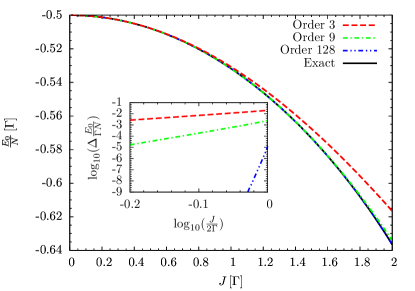
Figure 1: (Color online) Ground state energy per site as function of $J$. Comparison of the exact result to CUT results in various orders of $x=J/(2\Gamma)$. The inset shows the absolut difference between the exact result and the CUT calculation on a logarithmic scale. The critical point is located at $\log_{10}\left(\frac{J}{2\Gamma}\right)=0$.

V.2 Transverse magnetization

Next, we examine the transverse magnetization

$$M_{z}=-\frac{1}{N}\sum\limits_{j}\left\langle g\right|\sigma^{z}_{j}\left|g\right\rangle.$$ (34)

Here $\left|g\right\rangle$ denotes the ground state of the Hamiltonian which is mapped to the zero-particle state by the CUT. Note that the expression ‘transverse’ refers to the direction of the external field, which is the z-axis in our model. In the limit $J\rightarrow 0$, all spins are aligned along the external field, so that $M_{z}=1$ holds.

For $J>0$, the spins are perturbed by the antiferromagnetic interaction which reduces the transverse magnetization. To obtain $M_{z}$, we transform the observable $\sigma^{z}_{j}$ by the continuous unitary transformation to an effective observable. The operator of the transverse magnetization can be expressed by a string operator

$$\sum\limits_{j}\sigma^{z}_{j}(l=0)=T_{0}.$$ (35)

Due to this identity and the fact that the string algebra is closed under commutation, we know that the final effective observable can be written as a linear combination of string operators

$$\sigma^{z}(l) =o_{0}(l)T_{0}+\sum\limits_{n}\left[o_{n}^{+-}(l)\left(T_{n}^{+-}+\mathrm{h.c.}\right)\right.$$ (36a)

$$+\left.o_{n}^{++}(l)\left(T_{n}^{++}+\mathrm{h.c.}\right)\right].$$

None of the coefficients $o_{n}^{+-}$ and $o_{n}^{++}$ contribute to the vacuum expectation value. But they can not be omitted during the flow of the observable. The transverse magnetization after the CUT reads

$$M_{z}=o_{0}(\infty).$$ (37)

Due to this simple form of the observable very high orders can be reached again. The transverse magnetization calculated by the CUT is compared to the exact result in Fig. 2. As expected the results improve upon increasing order. The largest error occurs at the critical point where the transverse magnetization displays a singularity.

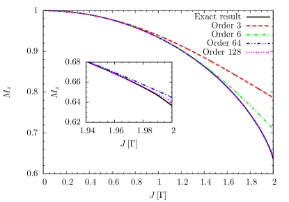
Figure 2: (Color Online) Transverse magnetization as a function of $J$. Comparison of the exact result with the CUT calculation. The inset shows a close view on the critical point $J=2{\Gamma}$.

V.3 Spectral weight

In this section, we discuss the CUT results for the momentum-integrated quasi-particle weight in the two diagonal channels $S^{xx}$ and $S^{yy}$. We use the CUT framework to calculate effective observables which renders an easy evaluation for the spectral weight possible in various quasi-particle channels, see also Ref. C. Knetter and G. S. Uhrig, 2004. The total spectral weight can be split according to

$$I^{\alpha\alpha}=\frac{1}{N}\sum\limits_{l}\left\langle\sigma_{l}^{\alpha}\sigma_{l}^{\alpha}\right\rangle=I_{1}+I_{2}+I_{3}+\dots,$$ (38)

where $I_{n}$ denotes the weight in the channel with $n$ quasi-particles in the system. Introducing the CUT framework results in

$$I^{\alpha\alpha}_{n}=\left\langle 0\right|\sigma_{n,\mathrm{eff}}^{\alpha}\sigma_{n,\mathrm{eff}}^{\alpha,\dagger}\left|0\right\rangle,$$ (39)

where $\sigma_{n,\mathrm{eff}}^{\alpha}$ denotes the part of the effective observable which annihilates $n$ quasi-particles. Since $\sigma^{x}$ and $\sigma^{y}$ create an odd number of spin flips, i.e., quasi-particles, and since the generator of the CUT preserves the parity of an observable, $S^{xx}$ and $S^{yy}$ consist of $1,3,5,\dots$ quasi-particle contributions. With the help of the sum rule $I^{{\alpha\alpha}}=1$, we can also check if our results are still valid for large values of $x$.

We emphasize that the local observables $\sigma_{l}^{x}$ and $\sigma_{l}^{y}$ transform into non-local operators under the Jordan-Wigner transformation which act on an infinite number of sites. Therefore, no easy analysis of these observables is possible in fermionic terms. An explicit evaluation requires either analytical mappings which enable an evaluation in the scaling region Vaidya and Tracy (1978) or extensive numerics in terms of Pfaffians whose dimensions grow linearly with the spatial range of the correlation Krones and Stolze (2011).

The problem of an infinite number of operators is avoided in the string operator basis (25). But the calculation remains cumbersome because the observables are not part of the string algebra and thus the structure of the effective observables is more complicated. This complicated structure prevents us from achieving very high orders, because the number of representatives to be tracked grows exponentially on increasing order. We are able to obtain results up to order $38$. Then the computational effort reaches its limit in the present implementation because the contributions to the differential equation system take more than $8$ GB of memory and the number of operators to track is larger than $7$ million.

First, we address $S^{xx}$ as function of $J$ for which results are depicted in Fig. 3. The CUT results are compared to the exact results from Ref. C. J. Hamer, J. Oitmaa, Z. Weihong and R.H. McKenzie, 2006. The one-particle contribution shows a very sharp drop for $J\to 2\Gamma$ with a singularity at the critical point. The CUT agrees very well with the exact results as long as the order of calculation is below the correlation length. Recall that the order is proportional to the range of the physical processes included in the calculation. For the calculation of effective observables within the string algebra this was no problem because large orders $>100$ could be achieved. But for the longitudinal correlations, we obtain only order 38 so that particularly sharp edges such as the one in the one-particle spectral weight are not captured. But the agreement improves on increasing order.

The spectral weight of the three-particle channel increases on approaching the critical point. Hence, spectral weight is transferred from the one-particle channel to higher quasi-particle channels. The one- and three-particle terms are the dominant contributions to the total spectral weight for the parameters investigated. But for $J>1.9$, the sum rule starts being violated in the CUT calculation. We attribute this violation to the calculation in finite order. It appears that the CUT calculation overestimates the one-particle contributions close to the critical point.

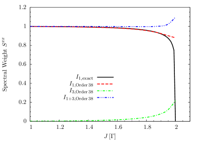
Figure 3: (Color Online) One-particle and three-particle spectral weight as function of the parameter $J$. Comparison of the exact expression for the one-particle weight (8a) with the CUT results.

Next, we investigate $S^{yy}$. This correlation is depicted in Fig. 4 in comparison to the exact result. Again, the one-particle contributions also vanish for $J\rightarrow 2\Gamma$. But the edge at the critical point is by far not as sharp as in $S^{xx}$ because more spectral weight is transferred to higher quasi-particle spaces for lower parameters $J$. The sum rule is again violated for $J>1.9\Gamma$ due to finite order errors.

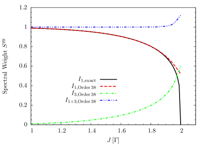
Figure 4: (Color online) One-particle and three-particle spectral weight as function of the parameter $J$. Comparison of the exact expression for the one-particle weight (8b) with the CUT results.

V.4 Equal-time structure factor

The momentum-resolved equal-time structure factor contains more information so that it is another interesting quantity

$$S^{\alpha\alpha}(Q)=\frac{1}{N}\sum\limits_{l,l^{\prime}}e^{-iQ(l-l^{\prime})}\langle\sigma_{l}^{\alpha}\sigma_{l^{\prime}}^{\alpha}\rangle.$$ (40)

For a single quasi-particle it is directly connected to the full DSF by Eq. (9) because there is no mixing between different quasi-particle spaces Knetter et al. (2001). Our first focus is $S_{1}^{xx}(Q)$. Within the CUT framework, this quantity can be computed from the effective observable $\sigma^{x}_{j,\mathrm{eff}}$ by Fourier transformation of the terms that exactly create one particle

$$S^{\alpha\alpha}_{n}(Q)=\left\langle 0\right|\sigma_{n,\mathrm{eff}}^{\alpha}(-Q)\sigma_{n,\mathrm{eff}}^{\alpha,\dagger}(Q)\left|0\right\rangle$$ (41)

where $n$ stands for the number of quasi-particles involved and $\alpha$ may take the values $x$ or $y$. In Fig. 5 we compare the CUT results to the exact expression (8a) for the parameters $J=\Gamma$, $J=1.5\Gamma$ and $J=1.9\Gamma$. The agreement is very impressive though it worsens upon approaching the critical point. For $J=\Gamma$ the DSF is essentially converged and the absolute errors are below $10^{-10}\Gamma^{-1}$. For $J=1.9\Gamma$ the error is below $10^{-3}\Gamma^{-1}$ for $Q<\pi/2$. For $Q>\pi/2$ the absolute error rises up to $10^{-1}\Gamma^{-1}$.

A closer analysis reveals that the largest absolute error occurs for all parameters at the wave vector $Q=\pi$. The DSF diverges at this point for $J\rightarrow 2\Gamma$. The relative error (not shown in the graphs) remains fairly constant over the whole Brillouin zone. Consequently our results differ from the exact ones found by Hamer et al. C. J. Hamer, J. Oitmaa, Z. Weihong and R.H. McKenzie (2006) by only about $1\%$ even close to the critical point at $J=1.9\Gamma$.

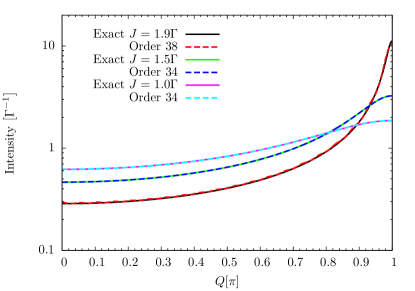
Figure 5: (Color Online) One-particle equal time structure factor $S_{1}^{xx}(Q)$ for the parameters $J=\Gamma$, $J=1.5\Gamma$ and $J=1.9\Gamma$. Comparison of the exact expression (8a) for the one-particle weight with the CUT results.

Finally, we consider $S_{1}^{yy}(Q)$. In Fig. 6 we compare the CUT results to the exact expression for the parameters $J=\Gamma$, $J=1.5\Gamma$ and $J=1.9\Gamma$. For $J=\Gamma$ the DSF is essentially converged and the absolute errors are below $10^{-10}\Gamma^{-1}$. This changes for rising parameter $J$. For $J=1.9\Gamma$ the error is below $10^{-2}\Gamma^{-1}$ for $Q<\pi/2$. For $Q>\pi/2$ the absolute error remains below $10^{-3}\Gamma^{-1}$. In contrast to the $S^{xx}$ channel, the lowest absolute error is located in the $S^{yy}$ channel at $Q\approx\pi$. This is can be easily understood because $S_{1}^{yy}(Q=\pi)$ constitutes a local minimum for all parameters $J$. Again, the relative error (not shown) remains essentially constant over the whole Brillouin zone.

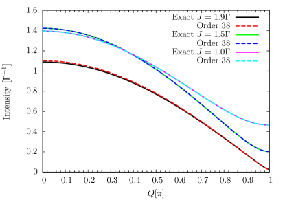
Figure 6: (Color online) One-particle equal time structure factor $S_{1}^{yy}(Q)$ for the parameters $J=\Gamma$, $J=1.5\Gamma$ and $J=1.9\Gamma$. Comparison of the exact expression (8b) with the CUT results.

VI Dynamic properties

In this section, we evaluate and present the dynamic results for the transverse field Ising model. Here, ‘dynamic’ refers to frequency dependent quantities. We deal with the dispersion in Sect. VI.1 and with the DSF in general in Sect. VI.2 and its different channels in Sects.  VI.3 ($S^{zz}$), VI.4 ($S^{xx}$) and VI.5 ($S^{yy}$).

The general DSF is an important quantity because it is directly measurable in scattering experiments. Furthermore, dynamic correlations strongly depend on the model under study and often exhibit features which reveal the microscopic interactions in the Hamiltonian. Despite the fact that the TFIM is integrable, the calculation of dynamic correlations remains a difficult and complex problem.

VI.1 Dispersion

As before we were able to reach order 256 for the CUT calculation of the Hamiltonian. In particular, we obtain the hopping matrix elements up to a range of 256. For small parameters $J$, a low order calculation is sufficient to achieve a good agreement with the exact result. Closer to the critical point this changes distinctly, see Fig. 7, which makes higher order calculations necessary. For $J=1.9\Gamma$ the absolute error of the result in order 6 is below $0.01\Gamma$ for $q<\pi/2$ and below $0.1\Gamma$ for $q>\pi/2$. For the order 32 result, it is below $10^{-4}\Gamma$ for $q<\pi/2$ and below $10^{-3}\Gamma$ for $q>\pi/2$. For $J=2\Gamma$, the error of the order 32 result is below $10^{-3}\Gamma$ for $q<\pi/2$ and below $10^{-1}\Gamma$ for $q>\pi/2$. For the order 256 result, it is below $10^{-5}\Gamma$ for $q<\pi/2$ and below $10^{-3}\Gamma$ for $q>\pi/2$.

This behavior is expected because the excitations become more and more dispersive on increasing $J$. Consequently, hopping processes over larger and larger distances become more important. To include these physical processes we need higher orders because the maximum range we can describe directly corresponds to the order of calculation (for lattice constant equal to unity). Directly at the critical point the energy gap closes and the correlation length diverges concomitantly.

The calculation of the dispersion is worst in the vicinity of the critical wave vector $q=\pi$. We stress, however, that the value directly at $q=\pi$, the energy gap of the TFIM, is calculated exactly up to numerical errors below $10^{-10}\Gamma$. This is an accidental result because the energy gap happens to be a linear function of $J$ so that it is captured correctly by any perturbative approach in linear order and beyond, compare Eq. (4).

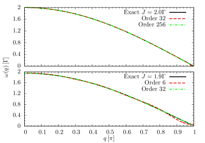
Figure 7: (Color online) Energy dispersion for $J=2.0\Gamma$ (top) and $J=1.9\Gamma$ (bottom). Comparison of the the CUT calculations to the exact results.

VI.2 Dynamic structure factor

The DSF at $T=0$ is linked to the imaginary part of the retarded Green function by the fluctuation-dissipation theorem at zero temperature Chandler (1987)

$$S^{\alpha\alpha}(\omega,Q)=-\frac{1}{\pi}\mathrm{Im}G^{\alpha\alpha}(\omega,Q).$$ (42)

At $T=0$, it is useful to write this Green function for $\omega>0$ as a resolvent

$$G^{\alpha\alpha}(\omega,Q) =\langle g|\sigma^{\alpha}(-Q)$$

$$\frac{1}{\omega-(H(Q)-E_{0})+i0^{+}}\sigma^{\alpha}(Q)|g\rangle$$ (43)

where $E_{0}$ is the ground state energy and

$$\sigma^{\alpha}(Q)=\frac{1}{\sqrt{N}}\sum\limits_{l}e^{iQl}\sigma^{\alpha}_{l}$$ (44)

is the Fourier transformed spin operator $\sigma_{l}^{\alpha}$.

In the CUT framework, we replace all operators by the effective operators and the ground state by the zero-particle state, i.e., the vacuum of quasi-particles

$$G^{\alpha\alpha}(\omega,Q) =\langle 0|S_{\mathrm{eff}}^{\alpha}(-Q)$$

$$\frac{1}{\omega-(H_{\mathrm{eff}}(Q)-E_{0})+i0^{+}}S_{\mathrm{eff}}^{\alpha}(Q)|0\rangle.$$ (45)

We evaluate the resolvent in Eq. (VI.2) by means of a Lanczos tridiagonalization yielding a continued fraction representation of the resolvent D. G. Pettifor and D. L. Weaire (1985); V. S. Viswanath and G. Müller (1994)

$$G^{\alpha\alpha}(\omega,Q)=\frac{b_{0}^{2}}{\omega-a_{0}-\frac{b_{1}^{2}}{\omega-a_{1}-\frac{b_{2}^{2}}{\ddots}}},$$ (46)

where the coefficients $a_{n}$ and $b_{n}$ are the matrix elements of the tridiagonal matrix of the effective Hamiltonian. We refer the reader to Appendices C and D where we explicitly calculate $S_{\mathrm{eff}}^{\alpha}(Q)|0\rangle$ as well as the action of the effective Hamiltonian for the Lanczos tridiagonalization. The continued fraction is terminated by a standard square-root terminator. This is appropriate for square root singularities at the band-edges.

Another piece of information that can be obtained from the sequences $\left\{a_{n}\right\}$ and $\left\{b_{n}\right\}$ are the exponents $\alpha$ and $\beta$ of the band-edge singularities, see Fig. 8. They are directly connected to the asymptotics D. G. Pettifor and D. L. Weaire (1985)

$$a_{n} =a_{\infty}+b_{\infty}\frac{\beta^{2}-\alpha^{2}}{2n^{2}}+\mathcal{O}\left(\frac{1}{n^{3}}\right)$$ (47a)

$$b_{n} =b_{\infty}+b_{\infty}\frac{1-2\alpha^{2}-2\beta^{2}}{8n^{2}}+\mathcal{O}\left(\frac{1}{n^{3}}\right).$$ (47b)

These relations allow us to obtain the band-edge singularities up to their signs by fitting

$$f(n)=C+\frac{D}{n^{2}}$$ (48)

to the continued fraction coefficients.

Figure 8: Qualitative sketch of the band-edge singularities in the DSF.

For two massive hardcore particles without interaction and with finite range hopping in one dimension the band-edge singularities are known to be $\alpha=\beta=1/2$, see for instance Refs. G. S. Uhrig and H. J. Schulz, 1996, 1998. We expect this behavior also to be true in the case of the TFIM because there is no interaction in the exact solution. In this case the relations (47a) and (47b) yield

$$a_{n} =a_{\infty}+\mathcal{O}\left(\frac{1}{n^{3}}\right)$$ (49a)

$$b_{n} =b_{\infty}+\mathcal{O}\left(\frac{1}{n^{3}}\right).$$ (49b)

We confirm this behavior in the two-particle case of the $S^{zz}$ channel in Sect. VI.3.

VI.3 $S^{zz}$ channel

Because the observable $\sigma^{z}$ stays local in the Jordan-Wigner representation of the TFIM the DSF in the $S^{zz}$ channel can be obtained analytically, see Eq. (7). The DSF in the $zz$ channel results from the two-particle continuum. Even for large parameters $J$, no weight is shifted towards four or more particle spaces. All dynamics induced by this observable is captured in the two-particle sector.

We emphasize that this fact holds as well in in the CUT treatment formulated in terms of the string operator algebra. The corresponding local operator $\sigma_{j}^{z}=O_{j,0}$ is element of the string algebra so that its effective observable after the CUT consists of a linear combination of string operators

$$\sigma_{j,\mathrm{eff}}^{z} =\sum\limits_{d}o_{j+d}O_{j+d,0}$$ (50)

$$+ \sum\limits_{d,n}\left[o_{j+d,n}^{+-}(O_{j+d,n}^{+-}+\mathrm{h.c.})+o_{j+d,n}^{++}(O_{j+d,n}^{++}+\mathrm{h.c.}\right])$$

where the maximum range $n$ is limited by the order of the calculation. We stress again that the operators $O_{j+d,0}$ and $O_{j+d,n}^{+-}$ do not create any excitations, while the operators $O_{j+d,n}^{++}$ create exactly two excitations. Thus, the vector $S_{\mathrm{eff}}^{\alpha}(Q)|0\rangle$ is only element of the zero- and of the two-particle Hilbert space. The same holds in the fermionic picture, where the operator $\sigma_{i}^{z}$ is a local density term which at most creates two fermionic excitations after the Bogoliubov diagonalization.

Concomitantly, very high orders can be reached also in the transformation of the local observable. Because we transform a non translational-invariant operator, we have to consider the positions $j+d$ and the starting site $j$ so that the number of terms increases quadratically with the order. But we are still able to achieve an order of $128$.

False color plots of the DSF obtained in this way are shown in Fig. 9 in order 128. The two-particle continuum is depicted in dependence of the total momentum $Q$ and the energy $\omega$. The overall intensity rises for larger parameters $J$. This stems from the decrease of the transverse magnetization which induces a shift of spectral weight from the zero-particle channel to the two-particle channel. Furthermore, we see that for small parameters $J/(2\Gamma)$ most of the weight is concentrated in the region $Q<\pi/2$ while the opposite behavior occurs for larger parameters $x$. Note the singularity inside the continuum on the right side of the Brillouin zone that separates two regions with low and high spectral weight, see the case $J=1.9\Gamma$. Knowing the exact expression (7) we can explain this singularity as van Hove singularity in the two-particle density-of-states. The two-particle energy $\omega(Q/2+q)+\omega(Q/2-q)$ displays a local maximum besides the global extrema as function of $q$, if $Q$ and $J$ are large enough.

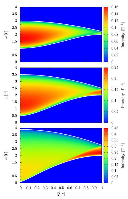
Figure 9: (Color online) The DSF $S^{zz}{(\omega,Q)}$ for the parameters $J=\Gamma$ (top), $J=1.5\Gamma$ (center) and $J=1.9\Gamma$ (bottom). The maximum range for the Lanczos algorithm is $d_{\mathrm{max}}=1000$ sites, the continued fraction was evaluated to a depth of $50$ and then terminated by the square root terminator. The color indicates the spectral density, see legend to the right. The upper and lower edge of the two-particle continuum are indicated by white lines.

We want to investigate more profoundly how the CUT calculation differs from the exact calculation by examining the DSF for fixed parameters $J$ and total momentum $Q$. Fig. 10 shows $S^{zz}{(\omega,Q)}$ for $J=1.5\Gamma$ and $J=1.9\Gamma$ and for the momenta $Q=0$, $Q=\pi/2$ and $Q=\pi$ calculated by the CUT in order 128 in comparison to the exact result. Note the excellent agreement for all parameters and momenta. The form of the DSF is very close to a half ellipse for low values of $J$ because the continued fraction coefficients converge very quickly towards their final values $a_{\infty}$ and $b_{\infty}$. For large $J$ more spectral weight is concentrated at the lower band-edge which we attribute to a complex interplay between momentum and energy conservation. For the parameters $J=1.9$ and $Q=\pi/2$, one clearly sees the singularity inside the continuum of the DSF which is the above mentioned van Hove singularity from a local maximum.

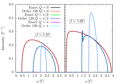
Figure 10: (Color online) DSF $S^{zz}{(\omega,Q)}$ for the parameters $J=1.5\Gamma$ (left) and $J=1.9\Gamma$ (right) for three total momenta $Q$. The maximum range for the Lanczos algorithm is $d_{\mathrm{max}}=4000$ sites, the continued fraction was evaluated to a depth of $100$ and then terminated by the square root terminator.

A detailed analysis shows that the error is lower in the middle of the continuum than at the band-edge singularities. This is expected due to the strong change of the DSF at the edges. On average, the error is below $10^{-6}\Gamma^{-1}$ even for large parameters $J$. At the band-edges the error can rise up to $10^{-3}\Gamma^{-1}$. We presume that the errors are mainly due to inaccuracies in the Lanczos tridiagonalization and due to the limited maximum range in the transformation of the observable by the CUT. Nonetheless the errors are still very small and justify our approach.

Next, we investigate how the continued fraction coefficients approach their limiting values. Thereby, we estimate the exponents of the band-edge singularities according to Eqs. (47a) and (47b). The continued fraction coefficients for the case $J=1.5\Gamma$ and total momenta $Q=0$ and $Q=\pi/2$ are shown in Fig. 11. The coefficients for the case $Q=0$ approach their limit exponentially. Therefore we know by Eqs. (47a) and (47b) that both exponents take the value $1/2$.

For the case $Q=\pi/2$, the coefficients do not converge so rapidly. We fit them for this case versus $1/n^{2}$ to check if they display terms in $\mathcal{O}(1/n^{2})$. Both coefficients oscillate around the final value which can not be described by Eqs. (47a) and (47b). This again indicates that the exponents at the band-edges are $1/2$. We also checked other momenta and they support the assumption that all exponents are $1/2$ for the two-particle case as it has to be according to the fermionic analytical results. Thus, these findings corroborate the validity of our approach and analysis.

Figure 11: (Color online) Absolute difference between the continued fraction coefficients and their final values for the case $J=1.5\Gamma$ and total momenta $Q=0$ and $Q=\pi/2$.

VI.4 $S^{xx}$ channel

In Ref. C. J. Hamer, J. Oitmaa, Z. Weihong and R.H. McKenzie, 2006 Hamer et al. derived an analytic expression for the one-particle contribution for the longitudinal structure factors. To our knowledge no data is available in the literature for higher quasi-particle contributions away from the scaling region Vaidya and Tracy (1978). Here our approach is able to provide complementary quantitative knowledge.

Similar to the two-particle case $S^{zz}{(\omega,Q)}$, the three-particle case $S_{3}^{xx}{(\omega,Q)}$ consists of a continuum of states. We are limited to a maximum order $38$ due to the complicated structure of the local observable $\sigma^{x}$ which is not part of the closed string algebra. Overview plots for the DSF obtained by the CUT are found in Fig. 12. In these plots the three-particle continuum is depicted in dependence of total momentum $Q$ and the energy $\omega$.

The total weight rises on increasing $J$ because spectral weight is transferred from the one-particle sector to the higher quasi-particle channels. The same qualitative behavior is observed for dimerized spin chains and spin ladders, and related systems K. P. Schmidt, C. Knetter and G.S. Uhrig (2004); C. Knetter, K. P. Schmidt and G.S. Uhrig (2003); T. Fischer, S. Duffe and G. S. Uhrig (2011). In addition, we notice that most of the spectral weight is concentrated at momenta $Q<\pi/2$ for small parameters $J$. The weight slowly shifts for growing $J$ similar to the $S^{zz}$ case. For $J=1.9\Gamma$, most of the spectral weight is concentrated rather strongly at the lower band-edge of the continuum. The same tendency was found in the $S^{zz}$ case as well. Still the shape of the DSF in the $S^{xx}$ case differs strongly from a semi-ellipse in contrast to the $S^{zz}$ DSF.

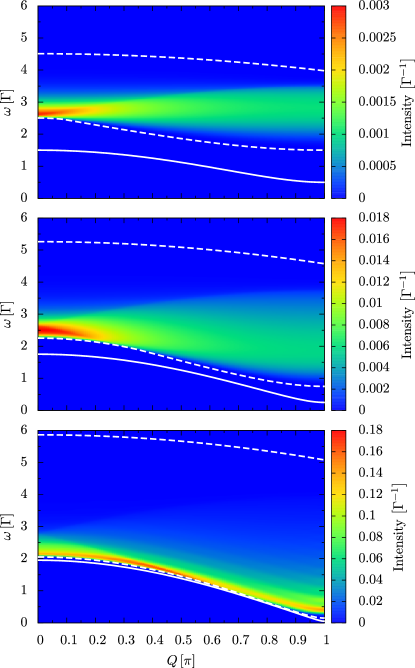
Figure 12: (Color online) The DSF $S_{3}^{xx}{(\omega,Q)}$ for the parameters $J=\Gamma$ (top), $J=1.5\Gamma$ (center) and $J=1.9\Gamma$ (bottom). The maximum range for the Lanczos algorithm is $d_{\mathrm{max}}=100$ sites, the continued fraction was evaluated to a depth of $50$ and then terminated by the square root terminator. The color indicates the spectral density, see legend to the right. The dispersion is indicated by the white solid line. The upper and lower edge of the three-particle continuum are indicated by white dashed lines. All results are computed in order 38.

A more quantitative investigation is shown in Fig. 13 where $S_{3}^{xx}$ is plotted for $J=1.9\Gamma$ and momenta $Q=0$, $Q=\pi/2$ and $Q=\pi$. It is confirmed that most of the spectral weight is concentrated at the lower band-edge for large values of $J$. For $Q=\pi$, a strong wiggling occurs which is to be attributed to the errors due to the calculation in finite order.

Figure 13: (Color online) DSF $S_{3}^{xx}{(\omega,Q)}$ for the parameter $J=1.9\Gamma$ for three chosen total momenta $Q$. The maximum range for the Lanczos algorithm is $d_{\mathrm{max}}=300$ sites, the continued fraction was evaluated to a depth of $100$ and then terminated by the square root terminator.

Next, we investigate the band-edge singularities in the three-particle case $S_{3}^{xx}{(\omega,Q)}$. As in the two-particle case, we use the relations (47a) and (47a) by fitting a $1/n^{2}$ power law to the continued fraction coefficients. An example is shown in Fig. 14

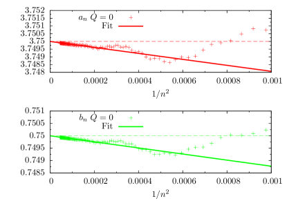
Figure 14: (Color online) Continued fraction coefficients for the case $J=1.5\Gamma$ and total momentum $Q=0$. The upper panel shows the coefficients $a_{n}$ and the lower panel shows the coefficients $b_{n}$. The limit values are indicated by horizontal lines. The red/green lines indicated linear fits in $1/n^{2}$; note the scale of the $x$-axis.

In contrast to the two-particle case, no exponential approach towards the limit values occurs. For all momenta, both $a_{n}$ and $b_{n}$ show a behavior proportional to $1/n^{2}$. We stress that the $\mathcal{O}(1/n^{3})$ terms are significant up to $1/n^{2}\approx 0.0002\,\Rightarrow n\approx 70$. The values for the band-edge singularities obtained from the fits are shown in Tab. 2.

$Q$	$\alpha$	$\beta$
0	2.5 $\pm$ 0.3	1.0 $\pm$ 0.2
$\pi/2$	3.0 $\pm$ 0.2	2.7 $\pm$ 0.2
$\pi$	3.0 $\pm$ 0.2	2.8 $\pm$ 0.1

Table 2: Exponents for the band-edge singularities of $S_{3}^{xx}{(\omega,Q)}$ for $J=1.5\Gamma$. The errors are determined from the fits using the Levenberg-Marquardt algorithm Levenberg (1944); Marquardt (1963).

For $Q=\pi$ and $Q=\pi/2$, both exponents are close to $3$ while for $Q=0$ the exponents differ and we deduce that $\alpha=2.5$ and $\beta=1$ holds. We stress, however, that the obtained exponents may still be affected by rather large numerical errors. In Ref. Kirschner, 2004, a general expression for the multi-particle band-edge singularities is derived for a simple one-dimensional model of hardcore bosons with nearest-neighbor hopping. The result reads

$$S_{n}\propto\omega^{\frac{n^{2}-3}{2}}\quad\mathrm{for}\,\,n>1,$$ (51)

, but close to the extrema of the dispersion. For the three-particle case, this yields $S_{n}\propto\omega^{3}$ which agrees well with our results for $Q=\pi$ and $Q=\pi/2$, but differs for $Q=0$. The discrepancy in the latter case may be due to the more complex structure of the dispersion in the effective Hamiltonian for the TFIM which includes longer range hopping processes.

VI.5 $S^{yy}$ channel

As in the $S^{xx}$ channel, the $S^{yy}$ channel consists of $1,3,5,\dots$ particle contributions. Overview plots for the three-particle DSF obtained by the CUT in order 38 are found in Fig. 15. In these plots, the three-particle continuum is plotted in dependence of the total momentum $Q$ and the energy $\omega$. For small $J$, the $S^{yy}$ channel looks similar to the $S^{xx}$ channel. The only difference is the absolute weight because the three-particle continuum in the $S^{yy}$ channel gains weight sooner,i.e., for smaller $J/(2\Gamma)$, than in the $S^{xx}$ channel.

For higher values of $J$, there are already qualitative differences between the $S^{xx}$ and the $S^{yy}$ channel. Most of the spectral weight is still concentrated at the lower band-edge of the continuum. No spectral weight is gained in the region of the critical wave vector $Q=\pi$ which constitutes a major difference to the $S^{xx}$ channel, see Fig. 12.

Figure 15: (Color online) DSF $S_{3}^{yy}{(\omega,Q)}$ for the parameters $J=\Gamma$ (top), $J=1.5\Gamma$ (center) and $J=1.9\Gamma$ (bottom). The maximum range for the Lanczos algorithm is $d_{\mathrm{max}}=100$ sites, the continued fraction was evaluated to a depth of $50$ and then terminated by the square root terminator. The color indicates the spectral density, see legend to the right. The dispersion is indicated by the white solid line. The upper and lower edge of the three-particle continuum are indicated by white dashed lines. All results are computed in order 38.

Scans of $S_{3}^{yy}$ at fixed $Q$ are shown in Fig. 16 for $J=1.9\Gamma$ and momenta $Q=0$, $Q=\pi/2$ and $Q=\pi$. For $Q\leq\pi/2$, most of the spectral weight is concentrated at the lower band-edge. This changes distinctly for $Q\geq\pi/2$, especially for $Q\approx\pi$. Here spectral weight is spread rather equally over frequency space. We also observe some wiggling which is due to finite order errors.

Figure 16: (Color online) DSF $S_{3}^{yy}{(\omega,Q)}$ for the parameter $J=1.9\Gamma$ for three chosen total momenta $Q$. The maximum range for the Lanczos algorithm is $d_{\mathrm{max}}=300$ sites, the continued fraction was evaluated to a depth of $100$ and then terminated by the square root terminator.

The values for the band-edge singularities obtained by fits as described before in the channels $S^{zz}$ and $S_{3}^{xx}$ are given in Tab. 3. They mostly equal those obtained for in the $S^{xx}$ channel within numerical errors. Only the case $Q=0$ differs. We deduce that $\alpha=3$ and $\beta=1$ holds for $S_{3}^{yy}$ generally.

$Q$	$\alpha$	$\beta$
0	2.9 $\pm$ 0.1	1.0 $\pm$ 0.1
$\pi/2$	2.9 $\pm$ 0.2	2.7 $\pm$ 0.2
$\pi$	2.9 $\pm$ 0.1	2.8 $\pm$ 0.2

Table 3: Exponents for the Band Edge Singularities for $S_{3}^{yy}(\omega,Q)$ for $J=1.5\Gamma$. The errors are determined from the fits using the Levenberg-Marquardt algorithm Levenberg (1944); Marquardt (1963).

VII Conclusion

Summarizing, we showed that the one-dimensional transverse field Ising model (1D TFIM) in the high field limit can be expressed in terms of string operators which form an algebra which is closed under commutation, which agrees with the previous finding by Jha and Valatin Jha and Valatin (1973). This property allowed us to solve the 1D TFIM in the high field limit to very high accuracy by continuous unitary transformations without resorting to the Jordan-Wigner transformation to non-interacting fermions. Note that the solution provided formally also covers the low field limit due to the duality of the model.

The only remaining restriction in the presented solution is the truncation in a given order $n$ in the ratio $x=J/(2\Gamma)$ of the Ising coupling $J$ to the field strength $\Gamma$. But due to the closure of the string algebra the number of terms to be tracked grows only linearly in the order $n$ so that very high orders up to $n=256$ can be achieved. Thus, accurate results for all practical purposes could be obtained. The order corresponds directly to the range of physical processes which are included if the lattice spacing is set to unity. We employed the recently developed deepCUT approach which is perturbatively correct in the targeted order and provides a robust extrapolation beyond this order H. Krull, N. A. Drescher and G. S. Uhrig (2012).

High orders are accessible for the Hamiltonian and all observables which belong to the string algebra. They cannot be obtained for observables which do not belong to the string algebra such as the longitudinal spin components. For this reason, the longitudinal components could be unitarily transformed only up to order $38$.

We gauged the results in computing various static properties such as the ground state energy, the transverse magnetization, and the one-particle contribution to the equal time structure factors $S_{1}^{\alpha\alpha}(Q)$ for $\alpha=x$ and $\alpha=y$. The first two quantities can be compared directly to the analytically accessible results via Jordan-Wigner transformation. The one-particle contribution to the equal time structure factors has been conjectured by Hamer and co-workers by series expansions and strongly underlined by the mapping to a two-dimensional classical Ising model for which the exact results are known C. J. Hamer, J. Oitmaa, Z. Weihong and R.H. McKenzie (2006).

Similarly, we computed dynamic quantities such as the one-particle dispersion and the momentum- and frequency-resolved diagonal dynamic structure factors. The dispersion and the transverse structure factor can again be gauged against the analytical result obtained in terms of non-interacting fermions. The longitudinal structure factors are much more difficult to address because their excitation operators are highly non-local in terms of the non-interacting fermions. While the one-particle contribution can be derived from the static one-particle structure factor and the exactly known dispersion there are no results for the next important three-particle contributions for general coupling $x\leq 1$. Only in the scaling region around the quantum phase transition results for the three-particle contributions in frequency domain exist Vaidya and Tracy (1978). Our results are reliable further away from the scaling region so that they are complementary to the existing information. The equation of motion approach pursued by Perk and Au-Yang Perk and Au-Yang (2009) provides information on the correlations in the time and real space domain. But so far no analysis with frequency and momentum resolution has been performed.

The presented theoretical three-particle data for the static and the dynamic structure factor provides predictions where in momentum and frequency space one can expect significant three-particle signal. This information may guide future experimental searches for many-particle contributions. Concretely, our results show that the $S^{yy}$ channel is considerably better suited for such searches than the $S^{xx}$ channel. In the $S^{xx}$ channel the single particle contributions dominates over the multi-particle contributions except very close to the quantum phase transition.

Moreover, we found that the spectral weight in the three-particle dynamic structure factors is concentrated close to the lower band-edge if the parameters are such that the system is not too far away from criticality. Further away from criticality the main response is rather featureless and hardly displays a dependence on the total momentum $Q$. Then the spectral weight is still concentrated close to the lower bandedge around $Q=0$, while it is spread out in the middle of the band around $Q=\pi$.

Our approach can be pursued further for all one-dimensional models of which the Hamilton operators can be expressed within the string algebra. Further investigations for other response functions are possible as well.

Appendix A Closure of the string algebra

Here we show that the string algebra is closed under commutation. This means that the commutator of two string operators can again be written as a linear combination of string operators. First, we show that on a chain two string operators commute if neither of their start-/end-operators are on the same site. Without loss of generality this means

$$0=\left[O_{j,n}^{\phi\epsilon},O_{l,m}^{\chi\xi}\right] ,\quad l>j,\quad l+m<j+n,$$ (52a)

$$0=\left[O_{j,n}^{\phi\epsilon},O_{l,m}^{\chi\xi}\right] ,\quad l>j,\quad l+m>j+n,$$ (52b)

$$0=\left[O_{j,n}^{\phi\epsilon},O_{l,m}^{\chi\xi}\right] ,\quad l>j+n,$$ (52c)

for $\phi,\epsilon,\chi,\xi\in\left\{+,-\right\}$. The last commutator (52c) is zero because operators acting on completely different sites always commute in a bosonic algebra. A simple calculation yields for the first commutator (52a)

$$\left[O_{j,n}^{\phi\epsilon},O_{l,m}^{\chi\xi}\right] \propto\left[\sigma_{l}^{z}\sigma_{l+m}^{z},\sigma_{l}^{\chi}\sigma_{l+m}^{\xi}\right],$$ (53a)

$$=\left[\sigma_{l}^{z}\sigma_{l+m}^{z},\sigma_{l}^{\chi}\right]\sigma_{l+m}^{\xi}$$ (53b)

$$+\sigma_{l}^{\chi}\left[\sigma_{l}^{z}\sigma_{l+m}^{z},\sigma_{l+m}^{\xi}\right],$$

$$=2\left\{(\chi)(\xi)\sigma_{l}^{\chi}\sigma_{l+m}^{\xi}-(\chi)(\xi)\sigma_{l}^{\chi}\sigma_{l+m}^{\xi}\right\},$$ (53c)

$$=0,$$ (53d)

using $\left[\sigma^{z},\sigma^{\chi}\right]=\chi 2\sigma^{\chi}$, $\sigma^{z}\sigma^{\chi}=\chi\sigma^{\chi}$ and $\sigma^{\chi}\sigma^{z}=-\chi\sigma^{\chi}$, if all operators act on the same site. Analogous calculations yield that (52b) holds as well.

The remaining contributions consist of commutators where either the start- and/or end-operators are on the same site. The start- and/or end-operators on the same site of two string operators need to be different because otherwise the identities $\sigma^{+}\sigma^{+}=\sigma^{-}\sigma^{-}=0$ imply a vanishing result. Explicit calculations yield for the non-vanishing commutators

$$\left[O_{j,n}^{\phi\epsilon},O_{j,m}^{-\phi\xi}\right] =\xi O_{j+m,n-m}^{\xi\epsilon},$$ (54)

with $m<n$ and

$$\left[O_{j,n}^{\phi\epsilon},O_{j+n,m}^{-\epsilon\xi}\right] =\epsilon O_{j,n+m}^{\phi\xi},$$ (55a)

$$\left[O_{j,n}^{\phi\epsilon},O_{j+n,0}\right] =-\epsilon 2O_{j,n}^{\phi\epsilon},$$ (55b)

$$\left[O_{j,n}^{\phi\epsilon},O_{j,n}^{-\phi-\epsilon}\right] =\frac{\phi}{2}O_{j,0}+\frac{\epsilon}{2}O_{j+n,0}.$$ (55c)

Explicit calculations for the translationally invariant string operators yield the following set of commutator relations for the case $n,m\in\mathbb{N}^{+},n<m$

$$\left[T_{n}^{++},T_{m}^{--}\right] =T_{n+m}^{+-}+T_{n+m}^{-+}-T_{m-n}^{+-}-T_{m-n}^{-+},$$ (56a)

$$\left[T_{n}^{++},T_{m}^{+-}\right] =T_{n+m}^{++}-T_{m-n}^{++},$$ (56b)

$$\left[T_{n}^{++},T_{m}^{-+}\right] =T_{n+m}^{++}-T_{m-n}^{++},$$ (56c)

$$\left[T_{m}^{++},T_{n}^{+-}\right] =T_{n+m}^{++}+T_{m-n}^{++},$$ (56d)

$$\left[T_{m}^{++},T_{n}^{-+}\right] =T_{n+m}^{++}+T_{m-n}^{++},$$ (56e)

$$\left[T_{n}^{++},T_{0}^{\phantom{-+}}\right] =-4T_{n}^{++},$$ (56f)

$$\left[T_{n}^{++},T_{m}^{++}\right] =0,$$ (56g)

and for the case $n=m$

$$\left[T_{m}^{++},T_{m}^{--}\right] =T_{2m}^{+-}+T_{2m}^{-+}+T_{0},$$ (57a)

$$\left[T_{m}^{++},T_{m}^{+-}\right] =T_{2m}^{++},$$ (57b)

$$\left[T_{m}^{++},T_{m}^{-+}\right] =T_{2m}^{++},$$ (57c)

$$\left[T_{m}^{++},T_{m}^{++}\right] =0,$$ (57d)

which are all linear combinations of string operators. Contributions with $n>m$ are also included by exchange of the arguments in the commutators. This concludes the derivation of the closure of the string algebra.

Appendix B Proof of infinite order flow equation

To prove the expression (33) we proceed in two steps. First, we show that all kinds of string operators of arbitrary range will be created during the flow. Next we show which contributions occur in the DES.

Our starting point for step one is the Hamiltonian of the TFIM in string operators in Eq. (IV). By induction we show that once we have a complete set of operators of maximum range $n$, $T_{0},T_{1}^{\pm\pm},T_{2}^{\pm\pm},\dots T_{n}^{\pm\pm}$ we can create a new complete set of operators of range $n+1$ by commutation with a string pair-creation-operator,

$$\left[T_{n}^{++},T_{1}^{--}\right] =T_{n+1}^{+-}+T_{n+1}^{-+}-T_{n-1}^{+-}-T_{n-1}^{-+},$$ (58a)

$$\left[T_{n}^{++},T_{1}^{+-}\right] =T_{n+1}^{++}-T_{n-1}^{++},$$ (58b)

$$\left[T_{n}^{--},T_{1}^{-+}\right] =-T_{n+1}^{--}+T_{n-1}^{--}.$$ (58c)

Thereby, we created the string operators of range $n+1$. Because the Hamiltonian in Eq. (IV) already comprises a complete set of range one we can deduce that all ranges $n\in\mathbb{N}^{+}$ will be created during the flow. Hence, we can conclude for the generator of the TFIM

$$\eta=\sum\limits_{n=1}^{\infty}t_{n}^{++}\left(T_{n}^{++}-T_{n}^{--}\right).$$ (59)

For step two we consider the relations in Eq. (56) and Eq. (57). We start with the contributions to the operator $T_{0}$. Such contributions are created only in the case $m=n$. For a given range $n$ there are two contributions from the commutators

$$\left[T_{n}^{++},T_{n}^{--}\right]=T_{0}+\dots,$$ (60a)

$$\left[T_{n}^{--},T_{n}^{++}\right]=-T_{0}+\dots,$$ (60b)

both with prefactor one. Note that $T_{n}^{++}$ and $T_{n}^{--}$ have the same prefactor up to a sign due to hermiticity/anti-hermiticity. Finally, these considerations yield

$$\partial_{l}t_{0}^{\phantom{+-}} =2\sum\limits_{n=1}^{\infty}\left(t_{n}^{++}\right)^{2}$$ (61)

for the flow equation for the prefactor of $T_{0}$.

Next, we consider the operator $T_{m}^{+-}$ and $T_{m}^{-+}$, respectively. They are created by two different kinds of commutators. For $k+l=m$

$$\left[T_{k}^{++},T_{l}^{--}\right]=T_{m}^{+-}+\dots,$$ (62a)

$$\left[T_{k}^{--},T_{l}^{++}\right]=-T_{m}^{+-}+\dots,$$ (62b)

and for $|k-l|=m$

$$\left[T_{k}^{++},T_{l}^{--}\right]=-T_{m}^{+-}+\dots,$$ (63a)

$$\left[T_{k}^{--},T_{l}^{++}\right]=T_{m}^{+-}+\dots,$$ (63b)

with prefactor one. Note that the operator $T_{m}^{-+}$ have the same prefactor as $T_{m}^{+-}$. These calculations yield

$$\partial_{l}t_{m}^{+-} =2\sum\limits_{k,l}^{k+l=m}t_{k}^{++}t_{l}^{++}-2\sum\limits_{k,l}^{|k-l|=m}t_{k}^{++}t_{l}^{++}.$$ (64)

Last we consider the operator $T_{m}^{++}$ and $T_{m}^{--}$, respectively. They are created by three different kinds of commutators. For $k+l=m$

$$\left[T_{k}^{++},T_{l}^{+-}\right]=T_{m}^{++}+\dots,$$ (65a)

$$\left[T_{k}^{++},T_{l}^{-+}\right]=T_{m}^{++}+\dots,$$ (65b)

for $|k-l|=m$

$$\left[T_{k}^{++},T_{l}^{+-}\right]=\mathrm{sgn}(k-l)T_{m}^{++}+\dots,$$ (66a)

$$\left[T_{k}^{++},T_{l}^{-+}\right]=\mathrm{sgn}(k-l)T_{m}^{++}+\dots,$$ (66b)

where the $\mathrm{sign}$ function stems from the different signs in the cases $\left[T_{n}^{++},T_{m}^{+-}\right]$ and $\left[T_{m}^{++},T_{n}^{+-}\right]$ in Eq. (56). Finally, the third case is given by

$$\left[T_{m}^{++},T_{0}\right]=-4T_{m}^{++}.$$ (67)

Now we can write down the complete flow equation for the prefactor $t_{m}^{++}$

$$\partial_{l}t_{m}^{++} =-4t_{m}^{++}t_{0}+2\sum\limits_{k,l}^{k+l=m}t_{k}^{++}t_{l}^{+-},$$

$$+2\sum\limits_{k,l}^{|k-l|=m}\mathrm{sgn}(k-l)t_{k}^{++}t_{l}^{+-},$$ (68a)

which concludes our derivation for the flow equation for infinite order.

Appendix C Calculation of $S_{\mathrm{eff}}^{\alpha}(Q)|0\rangle$

We start from Eq. (VI.2). To apply the Lanczos algorithm we need to calculate

$$S_{\mathrm{eff}}^{\alpha}(Q)|0\rangle.$$ (69)

We split the vector into its components of different particle number. For the two-particle structure factor the state

$$S_{\mathrm{eff}}\big{|}_{0}^{2}(Q)\left|0\right\rangle =\frac{1}{\sqrt{N}}\sum\limits_{r,d_{0},d_{1},j}e^{iQr}$$

$$\cdot s_{\mathrm{eff},j}^{d_{0},d_{1}}\left|r+d_{0},r+d_{0}+d_{1}\right\rangle,$$ (70)

with $d_{1}>0$ must be considered. The sum over $j$ addresses all operators that create an excitation at $r+d_{0}$ and another at $r+d_{0}+d_{1}$ which are different in their content of factors $\sigma^{z}_{i}$ at various sites. The index $j$ is used to distinguish them. In contrast, in a strict multi-particle representation there would be only one operator. Shifting the exponent by $d_{0}+d_{1}/2$, the center of mass, results in the expression

$$S_{\mathrm{eff}}\big{|}_{0}^{2}(Q)\left|0\right\rangle =\sum\limits_{d_{0},d_{1},j}e^{-iQ(d_{0}+d_{1}/2)}s_{\mathrm{eff},j}^{d_{0},d_{1}}$$

$$\cdot\underbrace{\frac{1}{\sqrt{N}}\sum\limits_{r}e^{iQ(r+d_{0}+d_{1}/2)}\left|r+d_{0},r+d_{0}+d_{1}\right\rangle}_{:=\left|Q,d_{1}\right\rangle},$$ (71a)

$$=\sum\limits_{d_{0},d_{1},j}\underbrace{e^{-iQ(d_{0}+d_{1}/2)}s_{\mathrm{eff},j}^{d_{0},d_{1}}}_{:=s_{\mathrm{eff},j}^{d_{0},d_{1}}(Q)}\left|Q,d_{1}\right\rangle,$$ (71b)

$$=\sum\limits_{d_{0},d_{1},j}s_{\mathrm{eff},j}^{d_{0},d_{1}}(Q)\left|Q,d_{1}\right\rangle,$$ (71c)

where we have introduced $\left|Q,d_{1}\right\rangle$ which is the Fourier transformation of a two-particle state with distance $d_{1}$.

For the three-particle structure factor the state

$$S_{\mathrm{eff}}\big{|}_{0}^{3}(Q)\left|0\right\rangle =\frac{1}{\sqrt{N}}\sum\limits_{r,d_{0},d_{1},d_{2},j}e^{iQr}s_{\mathrm{eff},j}^{d_{0},d_{1},d_{2}}$$

$$\cdot\left|r+d_{0},r+d_{0}+d_{1},r+d_{0}+d_{1}+d_{2}\right\rangle,$$ (72)

with $d_{1}>0$ and $d_{2}>0$ must be considered. Shifting the exponent by $d_{0}+2d_{1}/3+d_{2}/3$, the center of mass, results in the expression

$$S_{\mathrm{eff}}\big{|}_{0}^{3}(Q)\left|0\right\rangle =\sum\limits_{d_{0},d_{1},d_{2},j}e^{-iQ(d_{0}+2d_{1}/3+d_{2}/3)}s_{\mathrm{eff},j}^{d_{0},d_{1},d_{2}}$$

$$\cdot\underbrace{\frac{1}{\sqrt{N}}\sum\limits_{r}e^{iQ(r+d_{0}+2d_{1}/3+d_{2}/3)}\left|r+d_{0},r+d_{0}+d_{1},r+d_{0}+d_{1}+d_{2}\right\rangle}_{:=\left|Q,d_{1},d_{2}\right\rangle},$$ (73a)

$$=\sum\limits_{d_{0},d_{1},d_{2},j}\underbrace{e^{-iQ(d_{0}+2d_{1}/3+d_{2}/3)}s_{\mathrm{eff},j}^{d_{0},d_{1},d_{2}}}_{:=s_{\mathrm{eff},j}^{d_{0},d_{1},d_{2}}(Q)}\left|Q,d_{1},d_{2}\right\rangle,$$ (73b)

$$=\sum\limits_{d_{0},d_{1},d_{2},j}s_{\mathrm{eff},j}^{d_{0},d_{1},d_{2}}(Q)\left|Q,d_{1},d_{2}\right\rangle,$$ (73c)

where we introduced $\left|Q,d_{1},d_{2}\right\rangle$, which is the Fourier transformation of a three-particle state with distance $d_{1}$ between the first two particles and distance $d_{2}$ between the second two particles.

Appendix D Action of the effective Hamiltonian

To apply the Lanczos algorithm we need to know the action of the effective Hamiltonian on the two- and three-particle states, calculated in App. C. We stress that after the CUT there are no terms that violate particle-number conservation. We analyze the action of the operators $T_{0},T_{n}^{+-},T_{n}^{-+}$ separately. Starting with the simple operator $T_{0}$ yields

$$t_{0}(\infty)T_{0}\left|Q,d_{1}\right\rangle =t_{0}(\infty)T_{0}\frac{1}{\sqrt{N}}\sum\limits_{r}e^{iQ(r+d_{0}+d_{1}/2)}\left|r+d_{0},r+d_{0}+d_{1}\right\rangle,$$ (74a)

$$=t_{0}(\infty)(-N+4)\frac{1}{\sqrt{N}}\sum\limits_{r}e^{iQ(r+d_{0}+d_{1}/2)}\left|r+d_{0},r+d_{0}+d_{1}\right\rangle,$$ (74b)

$$=(E_{0}+4t_{0}(\infty))\left|Q,d_{1}\right\rangle.$$ (74c)

Next, we analyze the action of the operator $T_{n}^{+-}$

$$\sum\limits_{n}t_{n}^{+-}(\infty)T_{n}^{+-}\left|Q,d_{1}\right\rangle =\sum\limits_{n}(-1)^{n-1}t_{n}^{+-}(\infty)e^{iQn/2}\left|Q,d_{1}+n\right\rangle$$

$$+\sum\limits_{n<d_{1}}(-1)^{n-1}t_{n}^{+-}(\infty)e^{iQn/2}\left|Q,d_{1}-n\right\rangle$$ (75a)

$$+\sum\limits_{n>d_{1}}(-1)^{n}t_{n}^{+-}(\infty)e^{iQn/2}\left|Q,n-d_{1}\right\rangle,$$

and of the operator $T_{n}^{-+}$

$$\sum\limits_{n}t_{n}^{+-}(\infty)T_{n}^{-+}\left|Q,d_{1}\right\rangle =\sum\limits_{n}(-1)^{n-1}t_{n}^{+-}(\infty)e^{-iQn/2}\left|Q,d_{1}+n\right\rangle$$

$$+\sum\limits_{n<d_{1}}(-1)^{n-1}t_{n}^{+-}(\infty)e^{-iQn/2}\left|Q,d_{1}-n\right\rangle$$ (76a)

$$+\sum\limits_{n>d_{1}}(-1)^{n}t_{n}^{+-}(\infty)e^{-iQn/2}\left|Q,n-d_{1}\right\rangle.$$

Note the different signs of the second and third term due to the properties of the string operator.

Similarly to the two-particle state we examine the action of the effective Hamiltonian on the three-particle state. The simple operator $T_{0}$ yields

$$t_{0}(\infty)T_{0}\left|Q,d_{1},d_{2}\right\rangle =t_{0}(\infty)(-N+6)\left|Q,d_{1},d_{2}\right\rangle,$$ (77a)

$$=(E_{0}+6t_{0}(\infty))\left|Q,d_{1},d_{2}\right\rangle.$$ (77b)

Next, we analyze the action of the operator $T_{n}^{+-}$

$$\sum\limits_{n}t_{n}^{+-}(\infty)T_{n}^{+-}\left|Q,d_{1},d_{2}\right\rangle =\sum\limits_{n}(-1)^{n-1}t_{n}^{+-}(\infty)e^{iQn/3}\left|Q,d_{1}+n,d_{2}\right\rangle$$

$$+\sum\limits_{n<d_{1}}(-1)^{n-1}t_{n}^{+-}(\infty)e^{iQn/3}\left|Q,d_{1}-n,d_{2}+n\right\rangle$$

$$+\sum\limits_{n>d_{1}}(-1)^{n}t_{n}^{+-}(\infty)e^{iQn/3}\left|Q,n-d_{1},d_{2}+d_{1}\right\rangle$$ (78)

$$+\sum\limits_{n<d_{2}}(-1)^{n-1}t_{n}^{+-}(\infty)e^{iQn/3}\left|Q,d_{1},d_{2}-n\right\rangle$$

$$+\sum\limits_{d_{1}+d_{2}>n>d_{2}}(-1)^{n}t_{n}^{+-}(\infty)e^{iQn/3}\left|Q,d_{1}+d_{2}-n,n-d_{2})\right\rangle$$

$$+\sum\limits_{n>d_{1}+d_{2}}(-1)^{n-1}t_{n}^{+-}(\infty)e^{iQn/3}\left|Q,n-d_{1}-d_{2},d_{1})\right\rangle,$$

and of the operator $T_{n}^{-+}$

$$\sum\limits_{n}t_{n}^{+-}(\infty)T_{n}^{-+}\left|Q,d_{1},d_{2}\right\rangle =\sum\limits_{n}(-1)^{n-1}t_{n}^{+-}(\infty)e^{-iQn/3}\left|Q,d_{1},d_{2}+n\right\rangle$$

$$+\sum\limits_{n<d_{2}}(-1)^{n-1}t_{n}^{+-}(\infty)e^{-iQn/3}\left|Q,d_{1}+n,d_{2}-n\right\rangle$$

$$+\sum\limits_{n>d_{2}}(-1)^{n}t_{n}^{+-}(\infty)e^{-iQn/3}\left|Q,d_{1}+d_{2},n-d_{2}\right\rangle$$ (79)

$$+\sum\limits_{n<d_{1}}(-1)^{n-1}t_{n}^{+-}(\infty)e^{-iQn/3}\left|Q,d_{1}-n,d_{2}\right\rangle$$

$$+\sum\limits_{d_{1}+d_{2}>n>d_{1}}(-1)^{n}t_{n}^{+-}(\infty)e^{-iQn/3}\left|Q,n-d_{1},d_{1}+d_{2}-n\right\rangle$$

$$+\sum\limits_{n>d_{1}+d_{2}}(-1)^{n-1}t_{n}^{+-}(\infty)e^{-iQn/3}\left|Q,d_{2},n-d_{1}-d_{2}\right\rangle.$$

References

- Sachdev (2001) S. Sachdev, Quantum Phase Transitions (Cambridge University Press, 2001).
- Katsura (1962) S. Katsura, Phys. Rev. 127, 1508 (1962).
- Vidal (2007) G. Vidal, Phys. Rev. Lett. 98, 070201 (2007).
- H. Y. Yang and K. P. Schmidt (2011) H. Y. Yang and K. P. Schmidt, Europhys. Lett. 94, 17004 (2011).
- P. Jordan and E. Wigner (1928) P. Jordan and E. Wigner, Z. Phys. 47, 631 (1928).
- Niemeijer (1967) T. Niemeijer, Physica 36, 377 (1967).
- Pfeuty (1970) P. Pfeuty, Ann. of Phys. 57, 79 (1970).
- O. Derzhko and T. Krokhmalskii (1997) O. Derzhko and T. Krokhmalskii, Phys. Rev. B 56, 11659 (1997).
- O. Derzhko, T. Verkholyak, T. Krokhmalskii and H. Büttner (2006) O. Derzhko, T. Verkholyak, T. Krokhmalskii and H. Büttner, Phys. Rev. B 73, 214407 (2006).
- Perk (1980) J. H. H. Perk, Phys. Lett. A 79, 1 (1980).
- McCoy et al. (1983a) B. M. McCoy, J. H. H. Perk, and R. E. Shrock, Nucl. Phys. B 220, 35 (1983a).
- McCoy et al. (1983b) B. M. McCoy, J. H. H. Perk, and R. E. Shrock, Nucl. Phys. B 220, 269 (1983b).
- Müller and Shrock (1983) G. Müller and R. E. Shrock, Phys. Rev. Lett. 51, 219 (1983).
- Müller and Shrock (1984a) G. Müller and R. E. Shrock, Phys. Rev. B 29, 288 (1984a).
- Müller and Shrock (1984b) G. Müller and R. E. Shrock, Phys. Rev. B 30, 5254 (1984b).
- Müller and Shrock (1985) G. Müller and R. E. Shrock, Phys. Rev. B 31, 637 (1985).
- Perk and Au-Yang (2009) J. H. H. Perk and H. Au-Yang, J. Stat. Phys. 135, 599 (2009).
- Faddeev and Takhtajan (1981) L. D. Faddeev and L. A. Takhtajan, Phys. Lett. 85A, 375 (1981).
- Nagler et al. (1991) S. E. Nagler, D. A. Tennant, R. A. Cowley, T. G. Perring, and S. K. Satija, Phys. Rev. B 44, 12361 (1991).
- Dender et al. (1996) D. C. Dender, D. Davidović, D. H. Reich, C. Broholm, K. Lefmann, and G. Aeppli, Phys. Rev. B 53, 2583 (1996).
- Karbach et al. (1997) M. Karbach, G. Müller, A. H. Bougourzi, A. Fledderjohann, and K. H. Mütter, Phys. Rev. B 55, 12510 (1997).
- Knetter et al. (2001) C. Knetter, K. P. Schmidt, M. Grüninger, and G. S. Uhrig, Phys. Rev. Lett. 87, 167204 (2001).
- Schmidt and Uhrig (2005) K. P. Schmidt and G. S. Uhrig, Mod. Phys. Lett. B 19, 1179 (2005).
- Notbohm et al. (2007) S. Notbohm, P. Ribeiro, B. Lake, D. A. Tennant, K. P. Schmidt, G. S. Uhrig, C. Hess, R. Klingeler, G. Behr, B. Büchner, M. Reehuis, R. I. Bewley, C. D. Frost, P. Manuel, and R. S. Eccleston, Phys. Rev. Lett. 98, 027403 (2007).
- Christensen et al. (2007) N. B. Christensen, H. M. Rønnow, D. F. McMorrow, A. Harrison, T. G. Perring, M. Enderle, R. Coldea, L. P. Regnault, and G. Aeppli, Proc. Nat. Acad. Sciences 104, 15264 (2007).
- Jha and Valatin (1973) D. K. Jha and J. G. Valatin, J. Phys. A: Math. Nucl. Gen. 6, 1679 (1973).
- E. Lieb, T. Schultz and D. Mattis (1961) E. Lieb, T. Schultz and D. Mattis, Ann. Phys. (New York) 16, 407 (1961).
- Bogoliubov (1947) N. Bogoliubov, J. Phys. (USSR) 11, 23 (1947).
- Krones and Stolze (2011) J. Krones and J. Stolze, Phys. Rev. B 84, 052406 (2011).
- Lovesey (1987) S. W. Lovesey, Theory of Neutron Scattering from Condensed Matter (Oxford University Press, 1987).
- J. H. Taylor and G. Müller (1985) J. H. Taylor and G. Müller, Physica A 130, 1 (1985).
- C. J. Hamer, J. Oitmaa, Z. Weihong and R.H. McKenzie (2006) C. J. Hamer, J. Oitmaa, Z. Weihong and R.H. McKenzie, Phys. Rev. B 74, 060402 (2006).
- Wu et al. (1976) T. T. Wu, B. M. McCoy, C. A. Tracy, and E. Barouch, Phys. Rev. B 13, 316 (1976).
- Orrick et al. (2001) W. Orrick, B. Nickel, A. Guttmann, and J. Perk, J. Stat. Phys. 102, 795 (2001).
- Vaidya and Tracy (1978) H. G. Vaidya and C. A. Tracy, Physica A 92, 1 (1978).
- Wegner (1994) F. Wegner, Ann. Physik 506, 77 (1994).
- S. D. Głazek and K. G. Wilson (1993) S. D. Głazek and K. G. Wilson, Phys. Rev. D 48, 5863 (1993).
- S. D. Głazek and K. G. Wilson (1994) S. D. Głazek and K. G. Wilson, Phys. Rev. D 49, 4214 (1994).
- Mielke (1998) A. Mielke, Eur. Phys. J. B 5, 605 (1998).
- C. Knetter and G.S. Uhrig (2000) C. Knetter and G.S. Uhrig, Eur. Phys. J. B 13, 209 (2000).
- Fischer et al. (2010) T. Fischer, S. Duffe, and G. S. Uhrig, New J. Phys. 10, 033048 (2010).
- Drescher et al. (2011) N. A. Drescher, T. Fischer, and G. S. Uhrig, Eur. Phys. J. B 79, 225 (2011).
- Dusuel and Uhrig (2004) S. Dusuel and G. S. Uhrig, J. Phys. A: Math. Gen. 37, 9275 (2004).
- Heidbrink and Uhrig (2002) C. P. Heidbrink and G. S. Uhrig, Eur. Phys. J. B 30, 443 (2002).
- H. Krull, N. A. Drescher and G. S. Uhrig (2012) H. Krull, N. A. Drescher and G. S. Uhrig, Phys. Rev. B 86, 125113 (2012).
- C. Knetter, K. P. Schmidt and G. S. Uhrig (2003) C. Knetter, K. P. Schmidt and G. S. Uhrig, J. Phys. A: Math. Gen. 36, 7889 (2003).
- C. Knetter and G. S. Uhrig (2004) C. Knetter and G. S. Uhrig, Phys. Rev. Lett. 92, 027204 (2004).
- Chandler (1987) D. Chandler, Introduction to Modern Statistical Mechanics (Oxford University Press, 1987).
- D. G. Pettifor and D. L. Weaire (1985) D. G. Pettifor and D. L. Weaire, The Recursion Method and its Applications, Vol. 58 (Springer Verlag, Berlin, 1985).
- V. S. Viswanath and G. Müller (1994) V. S. Viswanath and G. Müller, The Recursion Method (Springer Verlag, Berlin, 1994).
- G. S. Uhrig and H. J. Schulz (1996) G. S. Uhrig and H. J. Schulz, Phys. Rev. B 54, R9624 (1996).
- G. S. Uhrig and H. J. Schulz (1998) G. S. Uhrig and H. J. Schulz, Phys. Rev. B 58, 2900 (1998).
- K. P. Schmidt, C. Knetter and G.S. Uhrig (2004) K. P. Schmidt, C. Knetter and G.S. Uhrig, Phys. Rev. B 69, 104417 (2004).
- C. Knetter, K. P. Schmidt and G.S. Uhrig (2003) C. Knetter, K. P. Schmidt and G.S. Uhrig, Eur. Phys. J. B 36, 525 (2003).
- T. Fischer, S. Duffe and G. S. Uhrig (2011) T. Fischer, S. Duffe and G. S. Uhrig, Europhys. Lett. 96, 47001 (2011).
- Levenberg (1944) K. Levenberg, Quarterly of Applied Mathematics 2, 164 (1944).
- Marquardt (1963) D. Marquardt, SIAM Journal on Applied Mathematics 11, 431 (1963).
- Kirschner (2004) S. Kirschner, Multi-particle spectral densities, Diplomarbeit, available at t1.physik.tu-dortmund.de/uhrig/diploma.html, Universität zu Köln (2004).