Vortex mechanics in planar nano-magnets

Abstract

A collective-variable approach for the study of non-linear dynamics of magnetic textures in planar nano-magnets is proposed. The variables are just arbitrary parameters (complex or real) in the specified analytical function of a complex variable, describing the texture in motion. Starting with such a function, a formal procedure is outlined, allowing a (non-linear) system of differential equations of motion to be obtained for the variables. The resulting equations are equivalent to Landau-Lifshitz-Gilbert dynamics as far as the definition of collective variables allows it. Apart from the collective-variable specification, the procedure does not involve any additional assumptions (such as translational invariance or steady-state motion). As an example, the equations of weakly non-linear motion of a magnetic vortex are derived and solved analytically. A simple formula for the dependence of the vortex precession frequency on its amplitude is derived. The results are verified against special cases from the literature and agree quantitatively with experiments and simulations.

The idea that particles are just stable non-linear excitations of fields is a cornerstone of modern field theoryMie1912a ; YangMills1954 ; Hooft2007 . The simplest such particle, the hedgehog, was discovered theoretically by SkyrmeS58 as a solution of non-linear field equations. Many similar configurations (topological solitons, or skyrmions) can be supported by a variety of fields, including those with a vectorial order parameter: magnetization, superfluid flow, or complex order parameters in superconductors. This makes condensed matter and, especially, magnetism a convenient setting for their study. In magnetism this subject gained new attention following direct experimental observations of magnetic vorticesSOHSO00 ; WWBPMW02 and skyrmion latticesMuhlbauerSkyrmionLattice ; yu2010realspaceobservation . Skyrmions are especially common in planar nano-magnets, where they can be concisely described by functions of complex variablesM10 , parametrized by the coordinates of their centers. Here a theoretical approach is presented for deriving the dynamical equations of motion of skyrmion’s generalized coordinates, which are equivalent (apart from the definition of the coordinates) to the Landau-Lifshitz dynamical equations for the magnetization vector fieldLL35 . It allows the application of classical mechanics to the complex non-linear problem of the dynamics of magnetic skyrmions, treating them like particles.

Magnetic textures of ferromagnetic thin films usually consist of magnetic domainsHubert_Shafer with largely uniform magnetization, separated by domain wallsHubert_book_walls , where the magnetization continuously rotates between the directions of adjacent domains. They were extensively studied in the framework of micromagnetics and are still interesting from both fundamental and applied points of view. The dynamics of these textures consists of the translation of magnetic domain walls and is traditionally described by the Thiele equationThiele1973 , which further assumes that the translation is steady. The possibility of such motion is a natural assumption for magnetic textures of infinite thin films.

In laterally confined nano-magnets the textures are very differentUP93 ; M01_solitons2 ; M10 , consisting of skyrmions (magnetic vortices and anti-vortices), some of which can be bound to the surfaceM01_solitons2 . There is no translational invariance, which makes direct application of the Thiele equation to these systems doubtful. It still can be applied to larger nano-magnetsHuber1982 ; GHKDB06 , where lateral confinement is less important, but to fully appreciate the specifics of nano-magnetism (magnetism on sub-micron scales) a different approach is needed.

Besides the Thiele equation there are other approaches to the problem of magnetization dynamics in laterally constrained magnets. One is based on volume averaging of the Landau-Lifshitz-Gilbert (LLG) equation in vector form and produces results in qualitative agreement with micromagnetic simulations and experimentsUK02 ; TCCGBT08 . But it leads to an underestimate of the texture mobilityTCCGBT08 and vortex precession frequencyUK02 , because the LLG equation is non-linear (due to the constraint on the length of the magnetization vector, masked when the equation is written in vector form) and its volume averaging (a form of linear superposition) is, generally, not justified. Consideration of spin-waves on a magnetic vortex backgroundISMW98 ; ZIPC05 does reproduce the translation of the magnetic vortex and predicts higher-energy spin-wave modes, but is limited to linear consideration of small vortex displacements only. Including higher order terms in the deviation of the magnetization from the (magnetic vortex) background is not only mathematically hard, but also bound to have difficulties reproducing the complicated non-linear motion of the multi-vortex texture, which may completely depart from the original static background. The non-uniform background also makes it difficult to deal with non-local dipolar forces, which is the reason why in many of such works (Refs ISMW98, ; ZIPC05, in particular) the dipolar interaction is replaced by a local in-plane anisotropy, making the equations partial differential (instead of integral partial differential). This approximation is justified in the limit of vanishing thickness of the nano-element, but quantitative agreement with experiments and simulations in a wide range of geometries is possible only when the magnetostatic interaction is fully accounted for.

Here an approach to magnetization dynamics in planar nano-dots is proposed. It is a collective-variable theory, capable of dealing with complex multi-vortex configurations (fully describing the relative motion and deformation of the constituent vortices). Its only approximation lies in the definition of collective variables, which are just arbitrary parameters in a complex function of a complex variable. Given such a function, the approach produces a system of ordinary differential equations (ODEs) of motion (with no integral terms even in the presence of magnetostatic interaction) for these variables. It assumes neither translational invariance nor steady-state motion and is fully capable of describing non-linear dynamics (if one can solve the resulting non-linear ODEs). The external field and other potential energy terms can be easily added without sacrificing simplicity (the dynamical equations still remain ODEs). It also allows the inclusion of phenomenological dissipation, akin to Gilbert’s damping term in the LLG equation. As an illustration, the equations of motion for linear and weakly non-linear magnetic vortex dynamics in circular nano-dots are derived and solved. As a check, the well-known analytical result for the vortex precession frequency (originally obtained by solving the Thiele equation) is then recovered in the limiting case of large dots.

The original motivation for this work comes from a recently published description of low-energy (single- and multiple-vortex) magnetic configurations in planar nano-dots of arbitrary shape in terms of functions of a complex variableM10 . The present approach can be thought of as a way to “animate” these configurations by making them move in accordance with LLG dynamics. Despite this, one may easily generalize it to other sets of trial functions without a substantial sacrifice in simplicity.

The usual starting point for consideration of magnetization dynamics is the LLG equationLL35 . It is well suited for numerical computations, but is not good for analytical ones. This is because the non-uniform effective field in the LLG approach, around which the magnetization vectors precess, depends, in turn, on the whole magnetization vector field (if the dipolar interaction is properly taken into account). This makes it a non-linear integral partial differential equation, which is extremely hard to solve analytically. Therefore, instead of the LLG equation, let us go deeper and consider, as a starting point, the kinetic Lagrangian density, which was first introduced by DöringDoering48 :

$$\tau=-\frac{M_{S}}{\gamma}\left(\cos\theta-\cos\theta_{0}\right)\frac{\partial\varphi}{\partial t},$$ (1)

where $\theta$ and $\varphi$ are the polar and azimuthal angle of the magnetic moment $\vec{M}$ in a spherical coordinate system, $t$ is time, $\gamma\simeq 1.76\times 10^{11}\mathrm{rad}/(\mathrm{s}\,\mathrm{T})$ is the gyromagnetic ratio, $M_{S}$ is the saturation magnetization, and $\theta_{0}$ is a constant. The parametrization of $\vec{M}$ via spherical angles conveniently satisfies the constraint $|\vec{M}|=M_{S}$, leaving only two of its components independent (and bounded). The system of two Euler-Lagrange equations for the extremum of the corresponding action over $\theta$ and $\varphi$ with additional time-independent potential energy terms subtracted, is equivalent to the Landau-Lifshitz equationDoering48 ; Hubert_book_walls . The equations do not depend on $\theta_{0}$, which can be used to ensure that $\tau$ is zero at the boundary of the magnet.

The collective variable approach is then similar to the Ritz methodRitz09 of solving boundary value problems: first, one selects a trial function, parametrizing a wide set of possible solutions, and then finds the values of the parameters giving the correct answer (extremalizing a certain functional, as per the variational principle). The Ritz method in its original formulation finds wide applications in micromagnetics for solving static problems. Dynamics is not much different. One may look for the extremum of action of the full Lagrangian, including the kinetic and potential energy, parametrized by a certain set of scalar parameters. The condition for this extremum produces dynamical equations for the parameters, allowing computation of their evolution in time.

While the above general recipe is applicable to an arbitrary choice of trial functions, to make further consideration more specific, let us focus on a particular very general familyM10 . Consider a cylinder, shown in Fig. 1, made of soft ferromagnetic material, with a Cartesian coordinate system, chosen in such a way that the axis $Z$ is perpendicular to the cylinder face ${\cal D}$, which is not necessarily circular.

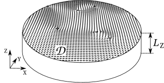
Figure 1: Illustration of a ferromagnetic cylinder with coordinate system axes (note that the present consideration is not limited to circular cylinders; the cylinder face ${\cal D}$ can have arbitrary shape). The arrows on top show a sample magnetic texture $\vec{m}(\vec{r})$ from Ref. M10, , containing vortices and anti-vortices. The positions of their centers are specified by collective coordinates.

If the cylinder is sufficiently thin, the equilibrium distribution of the magnetization vector $\vec{M}(\vec{r})$, $\vec{r}=\{X,Y,Z\}$, inside can be assumed to be independent of the coordinate $Z$. It can be conveniently parametrized by a complex function $w(z,\overline{z})$ of the complex variable $z=X+\imath Y$ (the overbar denotes the the complex conjugation, so that $\overline{z}=X-\imath Y$), expressing the normalized magnetization $\vec{m}=\vec{M}/M_{S}$ as

$$m_{X}+\imath m_{Y} = \frac{2w}{1+w\overline{w}}$$ (2)

$$m_{Z} = \pm\frac{1-w\overline{w}}{1+w\overline{w}},$$ (3)

which automatically satisfies the constraint $|\vec{m}|=1$. The sign of $m_{Z}$ controls the polarization of the vortex core: $m_{Z}=\pm 1$ at the vortex center.

In a flat cylinder the equilibrium static magnetization distributions can be represented as a combination of a soliton and a meronM10

$$w(z,\overline{z})=\left\{\begin{array}[]{ll}f(z)/c_{1}&|f(z)|\leq c_{1}\\ f(z)/\sqrt{f(z)\overline{f}(\overline{z})}&c_{1}<|f(z)|\leq c_{2}\\ f(z)/c_{2}&|f(z)|>c_{2},\end{array}\right.,$$ (4)

where $f(z)$ is an analytic [$\partial f(z)/\partial\overline{z}=0$] function of the complex variable $z$ and $c_{1}$ and $c_{2}$ are real constants.

In addition to the complex variable $z$ the function $w(z,\overline{z})$ usually depends on a number of other variables like $c_{1}$ and $c_{2}$, and others hidden inside $f(z)$. For example, the simplest translationally-invariant single magnetic vortex (Usov’s ansatzUP93 ) corresponds to

$$f_{\mathrm{U}}(z)=\frac{i(z-A)}{r_{V}},$$ (5)

with $c_{1}=1$ (absorbed into the vortex core radius $r_{V}$) and $c_{2}\rightarrow\infty$ in (4), since there are no anti-vortices. This magnetization distribution depends on the real parameter $r_{V}$ and the complex parameter $A$, which are the collective variables in this case. The parameter $A=a_{X}+\imath a_{Y}$ is the position of the vortex center. The problem, considered below, is how to find dynamical equations for these (and other similar) collective variables, assuming they are functions of time $t$, $r_{V}=r_{V}(t)$, $A=A(t)$.

The Landau-Lifshitz equation can also be written directly in complex notationSkrotskii84 . However, as discussed earlier, our starting point will be the kinetic part of the magnetic Lagrangian density (1), expressed through the collective variables and their time derivatives. In the complex notation its ingredients are

$$\cos\theta = \pm\frac{1-w\overline{w}}{1+w\overline{w}}$$ (6)

$$\exp(\imath\varphi) = \sqrt{\frac{w}{\overline{w}}}$$ (7)

$$\frac{\partial\varphi}{\partial t} = -\frac{\imath}{2}\frac{\partial}{\partial t}\ln\frac{w}{\overline{w}},$$ (8)

so that (1) can be rewritten as

$$\tau = \mp\frac{M_{S}}{\gamma}{\mathrm{Im}}\frac{1-w\overline{w}}{1+w\overline{w}}\frac{\dot{w}}{w},$$ (9)

where the dot over a variable denotes the time derivative and $w(z,\overline{z},t)$ from (4) depends on time $t$ via the collective variables in the trial function $f(z)$. The meron part of (4), as per our selection of $\theta_{0}=\pi/2$, gives no contribution to the kinetic Lagrangian, because $|w(z,\overline{z})|=1$ inside it, and therefore $\tau\sim m_{Z}\sim\cos\theta=0$.

To derive the dynamical equations the total Lagrangian is needed, which is the Lagrangian density integrated over the particle volume

$$T=\int_{{\cal D}\times L_{Z}}\tau\,{\mathrm{d}}^{3}\vec{r}=L_{Z}\int_{{\cal D}_{S}}\tau\,{\mathrm{d}}^{2}\vec{r},$$ (10)

where $L_{Z}$ is the cylinder’s thickness and ${\cal D}_{S}$ is the part of the cylinder’s face, occupied by soliton (4), for which $|f(z)|<c_{1}$ or $|f(z)|>c_{2}$. It can be simplified for arbitrary $f$ in (4) by noting that

$$\frac{\partial}{\partial t}\ln\frac{4w(t)\overline{w}(t^{\prime})}{(1+w(t)\overline{w}(t^{\prime}))^{2}}=\frac{1-w(t)\overline{w}(t^{\prime})}{1+w(t)\overline{w}(t^{\prime})}\frac{1}{w(t)}\frac{\partial w(t)}{\partial t}$$ (11)

where the variable $t^{\prime}$ is considered independent and does not take part in the differentiation. Interchanging the ${\mathrm{Im}}$ operation and the time derivative with the area integral (which is possible because the area element is real and integration is a linear operation) we arrive at the following expression for the total kinetic Lagrangian

$$T=\mp\frac{M_{S}L_{Z}}{\gamma}\left.{\mathrm{Im}}\frac{\partial}{\partial t}\!\!\int_{{\cal D}_{S}^{\prime}}\!\!\!\!\!\ln\frac{4\,w(z,t)\overline{w}(\overline{z},t^{\prime})}{(1+w(z,t)\overline{w}(\overline{z},t^{\prime}))^{2}}\,{\mathrm{d}}^{2}z\right|_{t^{\prime}\rightarrow t},$$ (12)

where for the purpose of calculating the area integral and differentiating it is assumed that all the collective variables inside $\overline{w}$ and the definition of the integration region ${\cal D}_{S}^{\prime}$ (note the prime) depend on the new independent time variable $t^{\prime}$, whereas inside $w$ they still depend on $t$ (only after differentiation is $t^{\prime}$ replaced by $t$). It was also noted that inside the soliton ${\cal D}_{S}$ the function $w$ is analytic and does not depend on $\overline{z}$, while its conjugate $\overline{w}$ does not depend on $z$. This formula can be checked directly. It can be further simplified if there are no boundary-bound vortices and anti-vortices. In this case it is possible to integrate (12) by parts, making use of Greene’s formula

$$\frac{1}{2\imath}\oint_{\partial{\cal D}}u(z,\overline{z})\,{\mathrm{d}}z=\iint_{\cal D}\frac{\partial u(z,\overline{z})}{\partial\overline{z}}\,{\mathrm{d}}^{2}z,$$ (13)

for any reasonably good function $u$, which yields

$$T=\pm\frac{M_{S}L_{Z}}{\gamma}\left[{\mathrm{Im}}\frac{\partial}{\partial t}\int_{{\cal D}_{S}^{\prime}}\overline{z}\frac{1-w\overline{w}}{1+w\overline{w}}\frac{1}{\overline{w}}\frac{\partial\overline{w}}{\partial\overline{z}}\,{\mathrm{d}}^{2}z\right]_{t^{\prime}\rightarrow t},$$ (14)

where the function arguments are omitted, but it is still assumed that all the collective variables inside $w$ depend on $t$ and all of them inside $\overline{w}$ and the definition of the region ${\cal D}_{S}^{\prime}$ depend on $t^{\prime}$.

The expression (12) (and (14) for the case of solitons fully contained inside the particle) is the main result of this paper. To derive the equations of motion for the collective variables $x_{i}(t)$, entering the trial function $f(\{x_{i}\},z)$, it is now sufficient to write down the full Lagrangian:

$$L(\{\dot{x}_{i}\},\{x_{i}\})=T(\{\dot{x}_{i}\},\{x_{i}\})-U(\{x_{i}\}),$$ (15)

where $U$ is the potential energy (including exchange, magnetostatic, and, possibly, other energy terms); and use it to derive the system of Euler-Lagrange equations

$$\frac{\,{\mathrm{d}}}{\,{\mathrm{d}}t}\frac{\partial L}{\partial\dot{x_{i}}}-\frac{\partial L}{\partial x_{i}}=0,$$ (16)

which extremize the corresponding action. This allows problems of (multi-) vortex dynamics to be treated as problems of classical mechanics. It is also worth noting that apart from restrictions, implied by a particular choice of $f$, in defining the collective variables $x_{i}$, the above consideration involves no approximations and corresponds to the solution of the LLG equation exactly. This is especially easy to see by considering a discrete magnet with each spin parametrized by the spherical angles $\theta_{ijk}$ and $\varphi_{ijk}$ and introducing discrete analogs of the static interactions (exchange, dipolar, etc) between the spins with finite differences instead of spatial derivatives. When all these spherical angles for each spin are chosen as independent variables, the equations of motion (16) in the continuum limit (when the number of spins goes to infinity, while the magnet volume is constant) coincide with the Landau-Lifshitz equation for $\theta(\vec{r},t)$ and $\varphi(\vec{r},t)$.

Let us now proceed with examples.

First, to illustrate that, as in classical mechanics, this theory may suffer from poor selection of trial functions, consider the dynamics of uniformly displaced magnetic vortex (5) with $r_{V}=\mathrm{const}$ and $A=A(t)$. One may readily check that all three expressions for the kinetic Lagrangian (10), (12), and (14) yield 0 in this case. This means that the Euler-Lagrange equations (16) reduce to conditions of static equilibrium, or (in the case of the potential energy, consisting of the exchange and magnetostatic terms) that such an undeformed vortex stays in the center of the cylinder. This is similar to the conclusion from micromagnetics that moving domain walls always have a different profile from that of stationary onesSchlomann73 . In some sense, one may say that such a modification of a magnetic texture (of a domain wall or a magnetic vortex) is the way in which it “remembers” that it is moving.

Let us now turn to a more complex trial function, describing vortex displacement without the formation of magnetic charges on the cylinder’s sideM01_solitons2 , which is a particular case of a more general class of trial functionsM10

$$f(z)=\imath\frac{z-(A+\overline{A}z^{2})}{r_{V}},$$ (17)

where again $r_{V}=\mathrm{const}$ and $A=A(t)=a_{X}(t)+\imath a_{Y}(t)$, $|A|<1/2$, is a complex pair of collective coordinates. The vortex center, where $f(z_{C})=0$, is not exactly at $z_{C}=A$, as in the case of a uniformly displaced vortex, but rather at $z_{C}=(1-\sqrt{1-4A\overline{A}})/(2\overline{A})$. While it is possible to change variables and write the equations of motion for $z_{C}(t)$ directly, let us illustrate one of the powers of the present approach, which is a great freedom in selecting the parametrization, and write them for $A(t)$. Also note that here the parameter $a$ in the original expression of Ref. M01_solitons2, is substituted by $-\imath A$, which makes the vortex center displacements coincide in phase with the complex parameter $A$. That is, real $A$ correspond now to real $z_{C}$. This again is a matter of convenience and does not change anything, since the parametrization can be arbitrary. The total Lagrangian up to the second order in $|A|$ from (14) and (15) with full account for the vortex core shape deformation is

$${\cal L}\!=\!\pm\kappa_{2}\left(a_{X}(t)\dot{a}_{Y}(t)\!-\!a_{Y}(t)\dot{a}_{X}(t)\right)-k_{2}\left(a_{X}^{2}(t)\!+\!a_{Y}^{2}(t)\right),$$ (18)

where ${\cal L}=L/(\mu_{0}M_{S}^{2}\pi L_{Z}R^{2})$ and $k_{2}$ are dimensionless and $\kappa_{2}=[1+r_{V}^{4}(4\ln\!2-3)]/(\gamma\mu_{0}M_{S})$ has units of seconds; $k_{2}$ is the second order expansion coefficient of the potential energy (consisting of exchange and dipolar terms). A constant zero-order potential energy term, equal to the equilibrium energy of the centered vortex, was omitted because it has no influence on dynamics of $a(t)$. The equations of motion (16) are

$$\kappa_{2}\dot{a}_{X}(t)\pm k_{2}a_{Y}(t) = 0,$$

$$\kappa_{2}\dot{a}_{Y}(t)\mp k_{2}a_{X}(t) = 0,$$ (19)

which, for initial conditions $a_{X}(0)=a_{0}$, $a_{Y}(y)=0$, have the following solution:

$$a_{X}(t) = a_{0}\cos(\omega t),$$

$$a_{Y}(t) = \pm a_{0}\sin(\omega t),$$ (20)

corresponding to the circular motion of the vortex around the dot center with frequency $\omega=\omega_{0}=k_{2}/\kappa_{2}$. It is important to note that the direction of vortex motion is not arbitrary. It depends on its core polarization, but not its chirality, since $T$ and $U$ are independent of the sign of $w$ or $f$. The vortices with $m_{Z}=-1$ at the center rotate clockwise, and the vortices with $m_{Z}=1$ counterclockwise. This is in full agreement with the simulations and experiments of Ref. Choe2004, , but in disagreement with its conclusions, since vortex chirality (included in “handedness”) plays no role in determining the direction of vortex rotation. This also allows us to guess that the vortex core polarization in the simulation of Ref. UK02, was positive, which is natural to assume, but was not specified by the authors. A similar polarization of the core can be guessed from Fig. 2 in Ref. GHKDB06, , but with significant uncertainty, since it is masked by low resolution of the measurement in the $Y$ direction, as discussed therein.

To make a more rigorous quantitative confirmation of the present theory, let us compute the rotation frequency of the magnetic vortex in the limit of large flat circular dots with $L_{Z}\ll R$ and $R\gg L_{E}$, where $L_{E}=\sqrt{C/\mu_{0}M_{S}^{2}}$ is the exchange length, $C$ is the exchange stiffness, and $R$ is the dot’s radius. In this case $r_{V}\ll 1$, and $\kappa_{2}\simeq 1/(\gamma\mu_{0}M_{S})$. The second order expansion of the energy of the vortex (17) with the vortex core neglected was published in Ref. MG02_JEMS, . If the exchange contribution of order $L_{E}/R\ll 1$ is also neglected in that expansion, the coefficient $k_{2}$ in large dots is fully determined by the energy of the volume magnetic charges MG02_JEMS . Converting to SI units, for the precession frequency we get

$$\nu = \frac{k_{2}}{2\pi\kappa_{2}}=\frac{\gamma\mu_{0}M_{S}}{\pi}\!\!\!\int\limits_{0}^{\infty}\frac{f_{\mathrm{MS}}(kg)}{k}\left[\int\limits_{0}^{1}\!rJ_{1}(kr)\,{\mathrm{d}}r\right]^{2}\!\!\!\!\,{\mathrm{d}}k,$$ (21)

$$\nu \simeq \gamma\mu_{0}M_{S}g\frac{2(2G-1)}{6\pi^{2}}$$ (22)

where $f_{\mathrm{MS}}(x)=1-(1-e^{-x})/x$, $g=L_{Z}/R\ll 1$ and $G\simeq 0.915\,966$ is Catalan’s constant. This expression [apart from measurement units and the value of the numerical constant in (22), which is exact here] coincides with the expression for the vortex frequency, obtained in Ref. GHKDB06, on the basis of the Thiele equation and quantitatively confirmed there by experiments on large dots. It is worth noting that in Ref. GHKDB06, different terms in the equation of motion correspond to different models: the dynamical term with time derivatives comes from the Thiele equation for uniform steady translation of magnetic texture, while the potential energy term assumes the non-uniform mode of vortex displacement from Ref. MG02_JEMS, . This is, strictly speaking, not consistent and works only because in large dots $r_{V}\ll 1$ and the dynamical term $\kappa_{2}\rightarrow 1$ becomes insensitive to the vortex core shape deformation. The derivation of the vortex precession frequency above is fully consistent and uses the same trial function for both the kinetic and potential energy terms.

Real magnets inevitably dissipate the energy of moving spins in the form of heat. But the Lagrangian formalism in its pure form does not include dissipation. It is added externally via the Rayleigh dissipation function $D$

$$D=\frac{1}{2}\sum_{i}\sum_{j}D_{ij}\dot{x_{i}}\dot{x_{j}},$$ (23)

which is then included into the right hand side of the Euler-Lagrange equations (16) as an additional term $-\partial D/\partial\dot{x_{i}}$. The matrix $D_{ij}$ consists of phenomenological dissipation coefficients. Judging from the abstract of the unpublished report by GilbertGilbert55 it is possible to speculate that the Lagrangian formalism was also his starting point and his dissipative term (whose full microscopic justification is still an open problemKambersky2007 ) has similar origins. Thus, $D_{ij}$ must be related to Gilbert’s phenomenological dissipation constant. This relation is, probably, best established by considering the energy balance in the system, but let us leave it for now as an open problem and treat $D_{ij}$ as independent phenomenological parameters. A choice of $D=d[\dot{a}_{X}(t)^{2}+\dot{a}_{Y}(t)^{2}]$ changes the solution (20) into

$$a_{X}(t) = a_{0}e^{-dk_{2}t/(d^{2}+\kappa_{2}^{2})}\cos\left[k_{2}t\kappa_{2}/(d^{2}+\kappa_{2}^{2})\right],$$

$$a_{Y}(t) = \pm a_{0}e^{-dk_{2}t/(d^{2}+\kappa_{2}^{2})}\sin\left[k_{2}t\kappa_{2}/(d^{2}+\kappa_{2}^{2})\right].$$ (24)

As one can see, as in the case of a linear oscillator, the vortex precession frequency starts to depend (slightly) on a (small) damping coefficient.

Finally, let us consider weakly non-linear vortex dynamics by taking into account the kinetic and potential energy terms, corresponding to the fourth order in $|A|$. Continuing the expansion of the kinetic Lagrangian (14) with the trial function (17) leads to the following expression:

$${\cal L} = \pm\{\kappa_{2}+\kappa_{4}[a_{X}^{2}(t)\!+\!a_{Y}^{2}(t)]\}\left[a_{X}(t)\dot{a}_{Y}(t)\!-\!a_{Y}(t)\dot{a}_{X}(t)\right]$$ (25)

$$-k_{2}\left[a_{X}^{2}(t)\!+\!a_{Y}^{2}(t)\right]-k_{4}\left[a_{X}^{2}(t)\!+\!a_{Y}^{2}(t)\right]^{2},$$

where $\kappa_{4}=2-r_{V}^{2}\{23+r_{V}^{2}[(6061-6397r_{V}^{2})/8-1152(1-r_{V}^{2})\ln 2]\}/(\gamma\mu_{0}M_{S})$ like $\kappa_{2}$ has units of seconds and $k_{4}$ is the next potential energy expansion coefficient. The corresponding equations of motion become non-linear, but they are solved exactly by (20) with

$$\omega=\frac{k_{2}+2a_{0}^{2}k_{4}}{\kappa_{2}+2a_{0}^{2}\kappa_{4}}\simeq\omega_{0}+2\frac{k_{4}\kappa_{2}-k_{2}\kappa_{4}}{\kappa_{2}^{2}}a_{0}^{2}+O(a_{0}^{4}).$$ (26)

As in other non-linear oscillators, the vortex rotation frequency becomes dependent on the rotation amplitude. Derivation of the expressions for $k_{2}$ and $k_{4}$ in the general case with full account for vortex core deformation is rather cumbersome and, together with the analysis of their dependence on the dot dimensions, will be the subject of another forthcoming presentation. Nevertheless, preliminary versions of these expressions are attached in the form of a MATHEMATICA file as a Supplemental Materialsuppfrequency . They can be used to compute vortex precession frequencies for various dot geometries, not covered here.

Limitations of the presented approach follow from its strengths. The results and the procedure are simple, but are just as good as the selected trial function. This is similar to the applications of the Ritz method to static problems of micromagnetics. Comparing the results obtained with different trial functions for a particular problem allows the one giving the most realistic description to be chosen. The quantitative basis for such a comparison can be the total action, corresponding to the evolution of the system between two known states. There are complications, however, due to the fact that the Lagrangian formalism prescribes that the action is stationary, but not necessarily minimal. Thus, development of a firm basis for comparison of different trial functions in the Lagrangian formalism might be an interesting possibility for future research with potential benefits across different branches of physics. In any case, more trial functions are considered, closer are the best ones to the exact analytical solution. Luckily, the family of trial functions from Ref. M10, is huge and can be further generalizedMG04 ; M06 , which facilitates such a competition. Vortex/anti-vortex pair nucleation is another problem, which requires a separate treatment. New vortices (changes in the topological charge) always come into the element through its boundary, a process well described by the considered family of trial functions in both the single-M01_solitons2 ; MG02_JEMS and multiple-M10 vortex cases. Vortex-antivortex annihilation is simple and corresponds to cancellation of monomials in the numerator and denominator of a rational complex trial functionM10 . Vortex-antivortex pair nucleation (without change in the total topological charge), however, introduces branching in the trial functions, where at some point in time and space additional monomials in the numerator and denominator of the rational function appear and spread out. While further evolution of the nucleated vortex-antivortex pair can be described by the presented approach directly, their initial nucleation requires the above-mentioned rigorous comparison between trial functions to detect when a trial function with more vortices and anti-vortices should replace the original one. Such branching points will have to be introduced into the dynamical process externally by showing that the total action of the process with nucleation and further evolution of the nucleated pair somewhere along the trajectory is lower than that with continued evolution of the original number of vortices. Consideration of branching might require an introduction of graph techniques similar to Feynman’s diagramsFeynman1949 .

Despite its limitations, the presented Lagrangian approach to linear and non-linear magnetic vortex dynamics can be directly applied to many interesting and useful problems of magnetism, such as magnetic vortex resonance in particles of various shapes (and influence of the particle shape on its frequency); the dynamics of vortex nucleation, when the “C”-shaped magnetization state transforms into a vortex dynamically; the dynamics of charged finite domain walls in nano-strips, which are well described by complex trial functionsM10 ; externally driven non-linear resonance; and chaos in unsaturated nano-magnets.

In conclusion, several equivalent alternative expressions for the kinetic Lagrangian (9), (10), (12), and (14) of an arbitrary trial function $f$, defining collective variables in (possibly multi-vortex) magnetic texturesM10 in flat nano-elements are derived. They allow non-linear equations of motion to be obtained for these variables similar to the ones in classical Lagrangian mechanics. Apart from the collective variable definition, this theory is exact and involves no additional approximations beyond those of the Landau-Lifshitz-Gilbert equation. It is validated here by considering magnetic vortex precession in a cylindrical nano-dot. In the limit of large flat dots its frequency coincides with experimental data and known theoretical estimations, based on the Thiele equationGHKDB06 . The question of the direction of the vortex rotation is elucidated. It is found to depend on vortex core polarization only and not on its chirality. Also, analytical solutions for vortex rotation in a dissipative magnet are derived (24); its frequency is decreased by damping. Finally, weakly non-linear rotation of the vortex is considered, allowing the relation (26) between its frequency and amplitude to be established via potential energy expansion coefficients. The expressions for the kinetic Lagrangian in (18) and (25) for the trial function (17) can be reused in other calculations, including evaluation of the time-dependent external field, spin torque, and other potential energy terms. One may expect them to be as simple as the examples above.

I would like to thank Vladimir N. Krivoruchko for reading the manuscript and many valuable suggestions.

References

- (1) G. Mie, Annalen der Physik 342, 511 (1912), ISSN 1521-3889
- (2) C. N. Yang and R. L. Mills, Phys. Rev. 96, 191 (Oct 1954)
- (3) G. ’t Hooft, in Philosophy of Physics, Part A., edited by J. Butterfield and J. Earman (Elsevier, 2007) pp. 661–730
- (4) T. H. R. Skyrme, Proc. Roy. Soc. A 247, 260 (1958)
- (5) T. Shinjo, T. Okuno, R. Hassdorf, K. Shigeto, and T. Ono, Science 289, 930 (2000)
- (6) A. Wachowiak, J. Wiebe, M. Bode, O. Pietzsch, M. Morgenstern, and R. Wiesendanger, Science 298, 577 (2002)
- (7) S. Mühlbauer, B. Binz, F. Jonietz, C. Pfleiderer, A. Rosch, A. Neubauer, R. Georgii, and P. Böni, Science 323, 915 (2009)
- (8) X. Yu, Y. Onose, N. Kanazawa, J. Park, J. Han, Y. Matsui, N. Nagaosa, and Y. Tokura, Nature 465, 901 (2010)
- (9) K. L. Metlov, Phys. Rev. Lett. 105, 107201 (2010)
- (10) L. D. Landau and E. M. Lifshitz, Physik. Z. Sowjetunion 8, 153 (1935)
- (11) A. Hubert and R. Schäfer, Magnetic Domains. The Analysis of Magnetic Microstructures (Springer, Berlin, 1998)
- (12) A. Hubert, Theorie der Domänenwände in geordneten Medien (Springer, Berlin-Heidelberg-New York, 1974)
- (13) A. A. Thiele, Phys. Rev. Lett. 30, 230 (1973)
- (14) N. A. Usov and S. E. Peschany, J. Magn. Magn. Mater. 118, L290 (1993)
- (15) K. L. Metlov, “Two-dimensional topological solitons in soft ferromagnetic cylinders,” (2001), arXiv:cond-mat/0102311
- (16) D. L. Huber, Phys. Rev. B 26, 3758 (1982)
- (17) K. Y. Guslienko, X. F. Han, D. J. Keavney, R. Divan, and S. D. Bader, Phys. Rev. Lett. 96, 067205 (2006)
- (18) N. Usov and L. Kurkina, J. Magn. Magn. Mater. 242–245 (2), 1005 (2002)
- (19) O. A. Tretiakov, D. Clarke, G.-W. Chern, Y. B. Bazaliy, and O. Tchernyshyov, Phys. Rev. Lett. 100, 127204 (2008)
- (20) B. A. Ivanov, H. J. Schnitzer, F. G. Mertens, and G. M. Wysin, Phys. Rev. B 58, 8464 (1998)
- (21) C. E. Zaspel, B. A. Ivanov, J. P. Park, and P. A. Crowell, Phys. Rev. B 72, 024427 (2005)
- (22) W. Döring, Z. Naturforschung 3a, 373 (1948)
- (23) W. Ritz, J. Mathematik 135, 1 (1909)
- (24) G. V. Skrotskii, Sov. Phys. Usp. 27, 977 (1984)
- (25) E. Schlömann, Appl. Phys. Lett. 19, 274 (1971)
- (26) S.-B. Choe, Y. Acremann, A. Scholl, A. Bauer, A. Doran, J. Stöhr, and H. A. Padmore, Science 304, 420 (2004)
- (27) K. L. Metlov and K. Y. Guslienko, J. Magn. Magn. Mater. 242–245, 1015 (2002)
- (28) T. Gilbert, Phys. Rev. 100, 1243 (1955)
- (29) V. Kamberský, Phys. Rev. B 76, 134416 (2007)
- (30) See Supplemental Material for Mathematica code computing potential energy expansion coefficients and vortex precession frequency.
- (31) K. L. Metlov and K. Y. Guslienko, Phys. Rev. B 70, 052406 (2004)
- (32) K. L. Metlov, Phys. Rev. Lett. 97, 127205 (2006)
- (33) R. P. Feynman, Phys. Rev. 76, 749 (1949)