Non-adaptive pooling strategies for detection of rare faulty items

Abstract

We study non-adaptive pooling strategies for detection of rare faulty items. Given a binary sparse $N$-dimensional signal $x$, how to construct a sparse binary $M\times N$ pooling matrix $F$ such that the signal can be reconstructed from the smallest possible number $M$ of measurements $y=Fx$? We show that a very low number of measurements is possible for random spatially coupled design of pools $F$. Our design might find application in genetic screening or compressed genotyping. We show that our results are robust with respect to the uncertainty in the matrix $F$ when some elements are mistaken.

I Introduction

Group testing [1, 2], also known as pooling in molecular biology, is designed to reduce the number of tests required to identify rare faulty items. In the most naive setting each item is tested separately and the number of tests is equal to the number of items. If, however, only a small fraction of the items are faulty, then the number of tests can be decreased significantly by creating “pools”, i.e. by including more than one item in one test and allowing each item to take part in several different tests. The main problem is how to design these pools such that their number is the smallest possible while allowing for a tractable, and robust to noise, reconstruction procedure.

In adaptive group testing the new pools are designed using the results of previous pools. However, many experimental situations require a non-adaptive testing where all pools must be specified without knowing the outcomes of other pools. Mainly two kinds of tests are relevant for practical applications. In Boolean group testing, each test outputs negative if it does not contain a faulty item and positive if it contains at least one faulty item. In linear group testing, each test outputs the number of faulty items. In practical applications the experimental constraints often require that the size of each pool is relatively small and one item does not belong to too many pools. In this paper we analyse the non-adaptive (single stage) pooling with linear tests and limited size of each pool.

A number of recent works have discussed a close relation between non-adaptive pooling with linear tests and compressed sensing [3, 4, 5, 6, 7, 8, 9, 10]. Here, we follow this direction of works and build on recent advances in compressed sensing that used spatially coupled design of measurements and permitted to decrease the number of measurements down to the information theoretical limit [11, 12, 13].

Our results are meant to find applications in various currently relevant problems e.g. genetic screening [4] or compressed genotyping [7]. In these applications, genes of several individuals are mixed together and one measures how many of the genes in a given pool are ”faulty”, e.g. related to certain genetic problem. This is usually done by introducing markers that attach to these faulty genes. The main source of noise in such experiments is that the marker does not attach, i.e. whereas one thought that a given gene belonged to a given pool, in reality it did not. We shall investigate the robustness of our results under this type of noise.

II Setting and related works

The non-adaptive pooling for detection of rare faulty items that we investigate is defined as follows: Consider a sparse binary $N$-dimensional vector $x$. Its components (items) are denoted by $x_{i}$, $i=1,\dots,N$. The vector is sparse: only $\rho N$ of the components are $x_{i}=1$ (faulty) and the others are $x_{i}=0$ (correct), with $\rho\ll 1$. A pool $a$ is a subset of components $a\subset\{1,\dots,N\}$. We denote $F_{ai}=1$ if component $i$ belongs to pool $a$ and $F_{ai}=0$ otherwise. The result of a pool/test

$$y_{a}=\sum_{i\in a}x_{i}=\sum_{i}F_{ai}x_{i}$$ (1)

is the number of faulty items in the pool. The goal is to design a smallest possible number $M$ of pools such that the vector $x$ can be reconstructed in a tractable way from the results of these pools $y=(y_{1},\dots,y_{M})$. In practice the result of a pool becomes often unreliable if the pool contains many items and also if one item belongs to many pools, because the sample corresponding to one item then needs to be split into many small pieces. We are hence interested in the case where the size of every pool $K_{a}$ is small (compared to $N$) and every item belongs to only a small number $L_{i}$ of pools.

This problem is reminiscent of compressed sensing [14, 15] which is designed to measure signals directly in their compressed form. In fact our problem is compressed sensing with the additional constraint that the signal is binary and with a sparse binary measurement matrix $F_{ai}$. We also consider matrix uncertainty: some elements assumed to be $F_{ai}\!=\!1$ are in fact $F_{ai}\!=\!0$ with probability $p$. The field of low-density parity check (LDPC) error correcting codes [16] provides information about sparse measurement matrices with which tractable reconstruction can be achieved. Indeed, the only difference between non-adaptive group testing with linear tests and LPDC is that the algebra is over integers in group testing instead of $GF(2)$ in LDPC. The spatially coupled pooling design we study here was first discovered and validated in the field of error correcting codes [17, 18, 19, 20].

The reconstruction algorithm that is most commonly used in compressed sensing and that has been also discussed several times for reconstruction in group testing and pooling experiments [3, 5, 6] is based on a linear relaxation of the problem to real signal components $0\leq x_{i}\leq 1$. One then minimizes the $\ell_{1}$-norm of the signal under the constraints $y=Fx$. This is a convex problem that can be solved efficiently using linear programing. In what follows we will use the $\ell_{1}$ reconstruction as a reference benchmark to demonstrate the improvement that can be achieved using our pooling design and the belief propagation based reconstruction.

The problem of non-adaptive group testing with linear tests, but with no constraints on the sparsity of the matrix $F$, is also known as the coin weighting problem [21, 22]. A detailed review of previous results can be found in [21]. It was shown [23] that, in the limit that interests us where $N\to\infty$, reconstruction is not possible with less than $M=(2\log{2})N/\log{N}$ tests. On the other hand a successful deterministic construction of the measurement matrix, together with a polynomial reconstruction algorithm, was found with $M=(2\log{2})N[1+o(1)]/\log{N}$ [24] measurements. As far as we know, however, the problem with a small (constant) number of items in every pool, as treated here, is still open.

Note that when the number of faulty items $R$ is much smaller than $N$, then another line of works should be considered. The best polynomial time non-adaptive algorithms known for the coin weighting problem then need $M=R\log_{2}{N}$ measurements [25]. Our approach is thus useful only in regimes where the number of faulty items is larger than $R>2(\log{2})^{2}N/\log^{2}{N}$. Another problem that is closely related to non-adaptive pooling as considered here is the sparse code division multiple access (CDMA) method [26, 27]; with the difference that the signal $x$ is not sparse and that there is usually a considerable Gaussian additive noise on the measurement vector $y$. The goal in CDMA is not to minimize the number of measurements $M$ (the number of chips), but to support the largest possible amount of noise. Spatial coupling was investigated for (dense) CDMA in [28, 29].

III Spatially coupled design of pools

The first design of pools (${\cal D}_{r}$) that we consider is based on a random construction. Each pool $a$ contains $K$ items. Each item $i$ belongs to $L$ pools. The assignment of items into pools is chosen uniformly out of all such possible ones. An example of a such random pooling matrix is plotted in Fig. 1 left.

The second design of pools (${\cal D}_{s}$), for which the total number of tests needed for successful reconstruction will be considerably smaller, is the “seeded” or “spatially-coupled” design, illustrated in Fig. 1 right. First, we divide the $N$ items into $B$ equally sized blocks. Pools are also divided into $B$ blocks, the first of them (the “seed”) being larger than the others. We will fix to $L$ the degree of all items, to $K_{s}$ the degree of pools in the first block, and to $K_{f}$ the degrees of pools in the other $B-1$ blocks. The size of the first block is then $M_{s}\!=\!NL/(K_{s}B)$, and that of the other blocks $M_{f}\!=\!NL/(K_{f}B)$. The overall under-sampling ratio is then $\alpha\!=\!L/(K_{s}B)+(B-1)L/(K_{f}B)$. When deciding connections between items and pools, we first connect randomly each pool to items in the block with the same index. Then we apply the following rewiring procedure: with probability $J$ for each edge (i.e. connection between an item and a pool), we chose randomly another edge whose item is in one of the $w$ previous blocks (and that has not been rewired yet) and switch the two edges. The details of this rewiring procedure do not change our results as long as a fraction of about $J$ of new connections is created up to distance $w$.

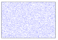
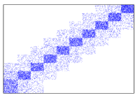
Figure 1: Left: Random pooling design, each blue point corresponds to an item $i$ belonging to a pool $a$. We took $N\!=\!2000$ items, $M\!=\!700$ pools, each item participates in $L\!=\!7$ pools, and each pool has $K\!=\!20$ items. Right: Seeded (or spatially coupled) design of pools, with $N\!=\!2000$ items, $M\!=\!490$ pools, $B\!=\!10$ blocks with $K_{s}\!=\!20$, $K_{f}\!=\!30$, $J\!=\!0.2$ and $w\!=\!2$.

IV Upper and lower bounds for number of pools

A simple lower bound on the number of necessary measurements $M$ can be obtained as follows: To reconstruct exactly the $N$-component signal of $R=\rho N$ non-zero components each possible configuration of the signal $x$ should correspond to a distinct result of the pools $y$. In other words the number of possible outcomes of the measurements must be larger than the number of possible signals. If $K$ denotes the number of items in each test this gives ${N\choose R}\leq(K+1)^{M}$. In the limit of large systems, and constant density of faulty items $\rho$ this gives $\alpha_{\rm LB}=H(\rho)/\log{(K+1)}$, where we use the entropy function $H(\rho)=-\rho\log{\rho}-(1-\rho)\log(1-\rho)$. Note that this lower bound holds also for adaptive pooling design.

We also derived a first moment upper bound on the critical ratio above which reconstruction is in principle possible for the random design (${\cal D}_{r}$). Calling $\cal N(\epsilon)$ the number of vectors $x$ compatible with the measurements $y$ at distance $1-\epsilon$ from the original signal, one obtains:

$$\mathbb{E}({\cal N(\epsilon)})\!\!\! = \!e^{N\Phi(\rho,\epsilon)}=e^{N[\alpha\log{P(\epsilon,K,\rho)}+H(\epsilon,\rho)]},\!$$ (2)

$$\text{where }H(\epsilon,\rho)\!\!\! = \!-\epsilon\rho\log{\epsilon\rho}-2(1-\epsilon)\rho\log{(1-\epsilon)\rho}$$

$$\!\!\!-(1-2\rho+\epsilon\rho)\log{(1-2\rho+\epsilon\rho)}-H(\rho),$$

$$\text{and }P(\epsilon,K,\rho)\!\!\! = \!\!\!\sum_{a=0}^{\frac{K}{2}}\frac{K!\left[1-2\rho(1-\epsilon)\right]^{K-2a}[(1-\epsilon)\rho]^{2a}}{(a!)^{2}(K-2a)!}\,.$$

When $\Phi(\rho,\epsilon)$ is negative everywhere except in the vicinity of $\epsilon\!=\!1$ then the linear system $y=Fx$ has only one solution that corresponds to the signal to be reconstructed. This leads to a threshold value $\alpha_{\rm UB}$ above which reconstruction is in principle possible. As we will see this upper bound is very close to the actual threshold. With $K\to\infty$, one can show that $\alpha_{\rm UB}=2\frac{H(\rho)}{\log K}$. For dense matrices $F$ with $K=N$, this is a tight bound, as mentioned in the context of coin weighting.

V Signal recovery algorithms

Knowing the set of tests or pools, i.e. the binary matrix $F$, and the measurement results $y$, one wants to reconstruct the signal. In compressed sensing the algorithms that achieve exact reconstruction with a smallest possible number of measurement are based on Bayesian inference, see [11, 12]. We thus adopt the same strategy here.

The probability distribution of observing measurements $y$ given the signal $x$ and set of pools $F$ is given as

$$P(y|x,F)=\prod_{a=1}^{M}{\sum_{i\in a}x_{i}\choose y_{a}}(1-p)^{y_{a}}p^{(\sum_{i\in a}x_{i}-y_{a})}$$ (3)

To estimate $P(x|y,F)$, with the use of Bayes rule $P(x|y,F)=P(y|x,F)P(x|F)/P(y|F)$, we need to assume some knowledge of statistical properties of the signal $x$. Denoting the fraction of non-zero elements $\rho$ we use a prior

$$P(x)=\prod_{i=1}^{N}\left[(1-\rho)\delta(x_{i})+\rho\delta(x_{i}-1)\right]$$ (4)

In compressed sensing it was argued [12] that for pooling matrices with random elements this assumption works as well for iid signal components as for correlated signals. Of course if an additional knowledge about the correlations in the signal were available it could be exploited and the performance improved further. We shall, however, not assume any such additional knowledge. The value of $x_{i}$ that minimizes the number of errors is obtained as the value that is more probable according to the marginal distribution for that element

$$\mu(x_{i})=\sum_{\{x_{j}\}_{j\neq i}}P(x|y,F).$$ (5)

To estimate these marginals we use the canonical belief propagation (BP) algorithm [30]. Following the usual derivation we introduce for each non-zero matrix element $F_{ai}$ two messages, $\chi^{i\to a}$ and $\psi^{a\to i}$, which are two-component vectors (normalized to $\chi^{i\to a}_{0}+\chi^{i\to a}_{1}=1$ and $\psi^{a\to i}_{0}+\psi^{a\to i}_{1}=1$), and we write iterative update equations for these as

$$\chi^{i\to a}_{x_{i}} = \frac{\rho^{x_{i}}(1-\rho)^{1-x_{i}}\prod_{b\in\partial i\backslash a}\psi^{b\to i}_{x_{i}}}{\rho\prod_{b\in\partial i\backslash a}\psi^{b\to i}_{1}+(1-\rho)\prod_{b\in\partial i\backslash a}\psi^{b\to i}_{0}}\,,$$ (6)

$$\psi^{a\to i}_{x_{i}} = \frac{1}{Z^{a\to i}}\sum_{B=y_{a}-x_{i}}^{K-x_{i}}{B+x_{i}\choose y_{a}}(1-p)^{y_{a}}p^{B+x_{i}-y_{a}}$$ (7)

$$\sum_{{\{{x_{j}}\}_{j\in\partial a\backslash i},\sum_{j}x_{j}=B}}\,\,\prod_{j\in\partial a\backslash i}\chi^{j\to a}_{x_{j}}\,.$$

In the iterative BP algorithm we initialize $\psi_{1}$ and $\chi_{1}$ as random numbers from the interval $(0,1)$ and update equations (6-7) till convergence. Note that the argument in equation (7) depends only on the sum of variables, it can thus be updated with the use of a convolution in $(K_{a}-1)^{2}/2$ steps (compared to the naive $2^{K_{a}-1}$ steps). Once convergence is reached the BP estimates of the marginal probabilities are computed by:

$$\chi^{i}_{x_{i}}=\frac{\rho^{x_{i}}(1-\rho)^{1-x_{i}}\prod_{a\in\partial i}\psi^{a\to i}_{x_{i}}}{\rho\prod_{b\in\partial i\backslash a}\psi^{a\to i}_{1}+(1-\rho)\prod_{a\in\partial i}\psi^{a\to i}_{0}}\,.$$ (8)

The BP inference of the item $i$ is then $x_{i}^{*}=1$ is $\chi^{i}_{1}>\chi^{i}_{0}$ and $x_{i}^{*}=0$ otherwise.

The iteration of message updates, starting from random messages, is the BP algorithm. It turns out that BP can also be used to analyse the optimal Bayes inference. For the purpose of this analysis one initializes BP messages to values corresponding to the true signal, and iterates the equations until convergence. In some region of parameters this will reach a different fixed point than the iterations of randomly initialized messages. The fixed point that corresponds to the result that would be achieved by the (exponentially costly) optimal Bayesian inference procedure is the one having the largest log-likelihood $\Phi$. The BP estimate of the log-likelihood, also called Bethe free energy, is given by

$$\Phi = \sum_{i}\log Z_{i}-\sum_{a}(K_{a}-1)\log Z_{a}\,,$$ (9)

$$Z_{i} = \rho\prod_{b\in\partial i\backslash a}\psi^{a\to i}_{1}+(1-\rho)\prod_{a\in\partial i}\psi^{a\to i}_{0}\,,$$

$$Z_{a} = \sum_{B=y_{a}}^{K}{B\choose y_{a}}\left(\frac{1}{p}-1\right)^{y_{a}}p^{B}\sum_{\begin{subarray}{c}\{{x_{j}}\}_{j\in\partial a}\\ \sum_{j}x_{j}=B\end{subarray}}\prod_{j\in\partial a}\chi^{j\to a}_{x_{j}}$$

In most practical situations the fraction of ”faulty” items $\rho$ is not known in advance. In such cases it can be learnt via expectation maximization learning, by iterating the following expression $\rho_{\rm new}=\sum_{i=1}^{N}\chi^{i}_{1}/N$, where the r.h.s. is evaluated using the previously estimated value of $\rho$.

VI Performance and phase diagrams

VI-A Noiseless case

Let us first investigate reconstruction of the signal for the random design ${\cal D}_{r}$. We are interested in the smallest possible ratio $\alpha_{c}=M_{c}/N$ for which exact reconstruction is still possible in the large $N$ limit. With the BP algorithm, exact reconstruction is possible if and only if $\alpha>\alpha_{BP}$. The threshold (or “phase transition”) $\alpha_{BP}$ is plotted in Fig. 3. We compare this value to the smallest possible ratio $\alpha_{\ell_{1}}$ for which the standard convex optimization approach, where one minimizes $|x|_{\ell_{1}}$ subject to $y=Fx$ and $0\leq x_{i}\leq 1$, provides exact reconstruction. We see in Fig. 3 that $\alpha_{\ell_{1}}$ is only slightly larger than $\alpha_{BP}$ for all range of $L$.

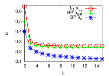
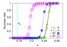
Figure 2: Left: The limit of performance for BP ($\alpha_{BP}$), $\ell_{1}$ minimization ($\alpha_{\ell_{1}}$) and the Bayes optimal inference ($\alpha_{c}$) for random design of pools. The values are obtained as averages over $20$ instances with $N=10^{4}$ items and density of faulty items $\rho=0.1$. Right: Fraction of exactly reconstructed signals using BP and $\ell_{1}$ reconstruction with random and seeded pools for $N=10^{4}$, $L=7$ and $\rho=0.1$. Data obtained from $100$ random instances. The seeded matrix has $B=20$ blocks, the first block (seed) has $K_{s}=20$, and following blocks have $K_{f}>20$ corresponding to different total values of $\alpha$. Fraction $J=0.4$ of links are connected to $w=2$ previous blocks.

Using the method explained in previous section, we have investigated the performance of Bayes optimal approach by evaluating the Bethe free energy $\Phi$. BP messages initialized on the true signal are fixed point in the absence of noise, corresponding to $\Phi=0$. Randomly initialized BP reaches the same fixed point at large values of $\alpha$, at $\alpha_{BP}$, $\Phi$ jumps discontinuously to negative values, meaning that there is no other signal with density $\rho$ satisfying all the tests. The log-likelihood then grows as $\alpha$ decreases and becomes positive at $\alpha_{c}$ below which there are other signals of density $\rho$ satisfying the tests and hence the true signal is undetectable. Above $\alpha_{c}$ the exactly evaluated Bayes-optimal inference would hence be able to reconstruct exactly the signal. The value of $\alpha_{c}$ is also plotted in Fig. 3 and we see that both $\ell_{1}$ and BP for random design of pools ${\cal D}_{r}$ are considerably suboptimal.

Using seeded pooling design improves BP performance by moving the ratio $\alpha$ above which BP is able to reconstruct exactly the signal down to the Bayes-optimal threshold $\alpha_{c}$. Several works have argued that quite generically when the system size $N$, the number of block $B$ and the interaction range $w$ go to infinity (in this order) BP with spatially coupled design is able to saturate the threshold $\alpha_{c}$ [18, 19, 20, 11, 12]. This statement applies also to our case. Here we investigate the performance of BP for seeded pooling design with realistic values of parameters $N$, $B$, $w$. In Fig. 2 right we plot the fraction of instances in which the signal was reconstructed exactly by $BP$ and $\ell_{1}$ for the random pooling design ${\cal D}_{r}$, and for the seeded design ${\cal D}_{s}$, with a set of parameters specified in Table I. Whereas $\ell_{1}$ performs basically the same for both designs, the performance of BP improves considerably in the seeded pooling scheme ${\cal D}_{s}$, for realistic values of the parameters. In Fig. 3 we summarize all our results for the noiseless case with $L=7$, and with a varying fraction of faulty items $\rho$. Let us also note that the Bayes-optimal transition for seeded matrices is not exactly equal to the one for random matrices, the two are, however, so close that the difference is not distinguishable in Fig. 3.

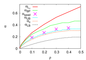
Figure 3: Lines are for random pooling design. From top: performance limit $\alpha_{\ell_{1}}$ for $\ell_{1}$, performance limit $\alpha_{BP}$ for BP, first moment upper bound on the Bayes-optimal inference, Bayes-optimal inference transition, and information theoretic lower bound. Number of items is $N=10^{5}$, each item is in $L=7$ pools. Data points mark the best performance we achieved with seeded matrices with $B=20$ and $w=2$, other parameters are listed in Table I.

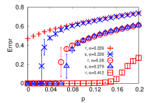
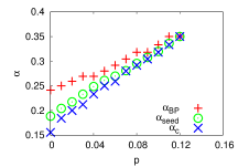
Figure 4: Left: Error (fraction of wrongly-reconstructed items) as function of noise strength $p$ for BP with random matrices and seeded matrices with $N=5\times 10^{4}$, $\rho=0.1$, $L=7$, and different $\alpha$ values, each point is averaged over $20$ instances. Seeded matrices have $B=10$ blocks, parameters are listed in Table I. Right: Spinodal, static transition and critical values for seeded matrices with $N=5\times 10^{4},\rho=0.1,L=7$. Seeded matrices have $B=20$ blocks, and parameters are listed in Table I.

VI-B Noisy case

We investigate now the robustness of our results to measurement-matrix noise. We denote by $p$ the probability that a matrix element $F_{ai}=1$ was in fact $F^{\rm true}_{ai}=0$, i.e. item $i$ did not contribute to the result of the test $a$. With nonzero values of $p$ and large system size $N\to\infty$ exact reconstruction is never possible, there is always a nonzero probability $p^{L}$ that a faulty item was never included in any measurement. However, for realistic sizes and small values of $p$ we may still obtain exact or close-to-exact reconstruction.

In the left part of Fig. 4 we plot the average error (fraction of wrongly reconstructed items) as a function of the noise strength $p$. We see that there is a critical value of $p$ above which the performance deteriorates significantly. This value is larger for the seeded pooling design than for the random pooling design. In the right part of Fig. 4 we then plot the critical values of ratio $\alpha$ as a function of noise strength $p$ for the random pooling design $\alpha_{BP}$, for the best seeded pooling design $\alpha_{\rm seed}$ that we found with realistic parameters, and for the Bayes optimal reconstruction $\alpha_{c}$. For $\alpha>0.35$ (for $\rho=0.1$, $L=7$) there is no longer a value of $p$ where the performance deteriorates sharply, instead the transition is smooth. Such a phase diagram is qualitatively similar to the one of compressed sensing with other types of noises, see e.g. [13, 31, 32].

TABLE I:

Parameters of seeded matrices in Fig. 3
$\rho$	$K_{s}$	$K_{f}$	$J$		$\rho$	$K_{s}$	$K_{f}$	$J$
0.1	20	39	0.1		0.2	15	27	0.1
0.3	13	22	0.1		0.4	11	21	0.1
Parameters of seeded matrices in Fig. 4 left
$\alpha$	$K_{s}$	$K_{f}$	$J$		$\alpha$	$K_{s}$	$K_{f}$	$J$
0.226	20	33	0.1		0.279	19	26	0.1
Parameters of seeded matrices in Fig. 4 right
$p$	$K_{s}$	$K_{f}$	$J$		$p$	$K_{s}$	$K_{f}$	$J$
0	20	39	0.1		0.01	18	36	0.2
0.02	16	34	0.3		0.03	19	31	0.3
0.04	18	29	0.3		0.05	24	27	0.3
0.06	15	27	0.4		0.07	14	26	0.4
0.08	19	24	0.3		0.09	19	23	0.4
0.1	20	22	0.4		0.11	20	21	0.4
0.12	20	20	0.4

VII Conclusion

We have studied non-adaptive pooling strategies for detection of rare faulty items. We have shown that the belief-propagation reconstruction algorithm, together with a seeded (spatially-coupled) design of the pools, leads to the best-known performance so far in the sense that it minimizes the number of measurements necessary for exact reconstruction in the noiseless case. Our results are very close to Bayes optimality and robust with respect to measurement noise corresponding to a faulty knowledge of the pools.

It is quite possible that this pooling design and its reconstruction algorithm will find applications in genetic screening. We note that our work can be extended to the case when the non-zeros items in the signal are real-valued. In this case the BP algorithm needs to be replaced by an AMP type of algorithm [33]. We are currently investigating this case for sparse measurement matrices.

References

- [1] D. Du and F. Hwang, Combinatorial group testing and its applications. World Scientific Publishing Company Incorporated, 1993.
- [2] ——, Pooling Design and Nonadaptive Group Testing. Singapore: World scientific, 2006.
- [3] A. Gilbert, M. Iwen, and M. Strauss, “Group testing and sparse signal recovery,” in Proc. of 42nd Asilomar Conf. on Signals, Systems, and Computers, 2009, pp. 1059 – 1063.
- [4] A. A. Y. Erlich, N. Shental and O. Zuk, “Compressed sensing approach for high throughput carrier screen,” in 47th Annual Allerton Conference on Communication, Control, and Computing, 2009. Allerton 2009., 2009, pp. 539 –544.
- [5] A. A. N. Shental and O. Zuk, “Rare-allele detection using compressed se(que)nsing,” 2009, arXiv:0909.0400.
- [6] ——, “Identification of rare alleles and their carriers using compressed se(que)nsing,” Nucleic Acids Research, vol. 38, 2010.
- [7] Y. Erlich, A. Gordon, M. Brand, G. Hannon, and P. Mitra, “Compressed Genotyping,” IEEE Trans. on Inform. Theory, vol. 56, pp. 706–723, 2010.
- [8] R. M. Kainkaryam, “Pooling designs for high-throughput biological experiments,” Ph.D. dissertation, University of Michigan, 2010.
- [9] B. Narayanaswamy, “Sparse measurement systems: Applications, analysis, algorithms and design,” Ph.D. dissertation, Carnegie Mellon University, 2011.
- [10] R. Mourad, “Designing pooling systems for high-throughput identifcation of biological interactions using compressed sensing,” Master’s thesis, American University of Beirut, 2012.
- [11] F. Krzakala, M. Mézard, F. Sausset, Y. Sun, and L. Zdeborová, “Statistical physics-based reconstruction in compressed sensing,” Phys. Rev. X, p. 021005, 2012.
- [12] D. L. Donoho, A. Javanmard, and A. Montanari, “Information-theoretically optimal compressed sensing via spatial coupling and approximate message passing,” in Proc. of the IEEE Int. Symposium on Information Theory (ISIT), 2012., 2011.
- [13] F. Krzakala, M. Mézard, F. Sausset, Y. Sun, and L. Zdeborová, “Probabilistic reconstruction in compressed sensing: algorithms, phase diagrams, and threshold achieving matrices,” Journal of Statistical Mechanics: Theory and Experiment, vol. 2012, no. 08, p. P08009, 2012.
- [14] E. J. Candès and T. Tao, “Decoding by linear programming,” IEEE Trans. Inform. Theory, vol. 51, p. 4203, 2005.
- [15] D. L. Donoho, “Compressed sensing,” IEEE Trans. on Inform. Theory, vol. 52, p. 1289, 2006.
- [16] R. G. Gallager, “Low-density parity check codes,” IEEE Trans. Inform. Theory, vol. 8, pp. 21–28, 1962.
- [17] A. Jimenez Felstrom and K. Zigangirov, “Time-varying periodic convolutional codes with low-density parity-check matrix,” Information Theory, IEEE Transactions on, vol. 45, no. 6, pp. 2181 –2191, 1999.
- [18] M. Lentmaier, A. Sridharan, J. D. J. Costello, and K. S. Zigangirov, “Iterative decoding threshold analysis for LDPC convolutional codes,” IEEE Trans. Inf. Theory, vol. 56, 2010.
- [19] M. Lentmaier, D. G. M. Mitchell, G. P. Fettweis, and D. J. Costello, Jr., “Asymptotically good LDPC convolutional codes with AWGN channel thresholds close to the Shannon limit,” in Proc. 6th Int. Symp. on Turbo Codes and Iterative Inf. Processing, 2010.
- [20] S. Kudekar, T. Richardson, and R. Urbanke, “Threshold saturation via spatial coupling: Why convolutional ldpc ensembles perform so well over the bec,” in Information Theory Proceedings (ISIT),, 2010, pp. 684–688.
- [21] N. H. Bshouty, “Optimal algorithms for the coin weighing problem with a spring scale,” in Conference on Learning Theory, 2009.
- [22] G. D. Marco and D. R. Kowalski, “Searching for a subset of counterfeit coins: Randomization vs determinism and adaptiveness vs non-adaptiveness,” Random Struct. Alg., 2012.
- [23] Erdős and A. Rényi, “On two problems of information theory,” Publ. Math. Inst. Hung. Acad. Sci., vol. 8, 1963.
- [24] B. Lindstrőm, “On a combinatory detection problem i,” Mathematical Institute of the Hungarian Academy of Science, vol. 9, 1964.
- [25] ——, “On b2-sequences of vectors,” Number Theory, vol. 4, 1972.
- [26] J. Raymond and D. Saad, “Sparsely spread cdma—a statistical mechanics-based analysis a,” Journal of Physics A: Mathematical and Theoretical, vol. 40, p. 12315, 2007.
- [27] D. Guo and C.-C. Wang, “Multiuser detection of sparsely spread cdma,” Selected Areas in Communications, IEEE Journal on, vol. 26, no. 3, pp. 421 –431, april 2008.
- [28] C. Schlegel and D. Truhachev, “Multiple access demodulation in the lifted signal graph with spatial coupling,” 2011, iEEE IT.
- [29] K. Takeuchi, T. Tanaka, and T. Kawabata, “Improvement of bpbased cdma multiuser detection by spatial coupling,” 2011, coRR, vol. abs/1102.3061.
- [30] J. Yedidia, W. Freeman, and Y. Weiss, “Understanding belief propagation and its generalizations,” in Exploring Artificial Intelligence in the New Millennium. San Francisco, CA, USA: Morgan Kaufmann, 2003, pp. 239–236.
- [31] J. Barbier, F. Krzakala, M. Mézard, and L. Zdeborová, “Compressed sensing of approximately-sparse signals: Phase transitions and optimal reconstruction,” in Proc. 50th Annual Allerton Conf. on Commun., Control, and Comp., 2012.
- [32] F. Krzakala, M. Mézard, and L. Zdeborová, “Compressed sensing under matrix uncertainty: Optimum thresholds and robust approximate message passing,” 2013, arXiv:1301.0901 [cs.IT].
- [33] D. L. Donoho, A. Maleki, and A. Montanari, “Message-passing algorithms for compressed sensing,” Proc. Natl. Acad. Sci., vol. 106, no. 45, pp. 18 914–18 919, 2009.