Analysing the Transverse Structure of the Relativistic Jets of AGN

Abstract

This paper describes a method of fitting total intensity and polarization profiles in VLBI images of astrophysical jets to profiles predicted by a theoretical model. As an example, the method is used to fit profiles of the jet in the Active Galactic Nucleus Mrk 501 with profiles predicted by a model in which a cylindrical jet of synchrotron plasma is threaded by a magnetic field with helical and disordered components. This fitting yields model Stokes $Q$ profiles that agree with the observed profiles to within the $1-2\sigma$ uncertainties; the $I$ model and observed profiles are overall not in such good agreement, with the model $I$ profiles being generally more symmetrical than the observed profiles. Consistent fitting results are obtained for profiles derived from 6 cm VLBI images at two distances from the core, and also for profiles obtained for different wavelengths at a single location in the VLBI jet. The most striking success of the model is its ability to reproduce the spine–sheath polarization structure observed across the jet. Using the derived viewing angle in the jet rest frame, $\delta^{\prime}\simeq 83^{\circ}$, together with a superluminal speed reported in the literature, $\beta_{app}=3.3$, yields a solution for the viewing angle and velocity of the jet in the observer’s frame $\delta\simeq 15^{\circ}$ and $\beta\simeq 0.96$. Although these results for Mrk501 must be considered tentative, the combined analysis of polarization profiles and apparent component speeds holds promise as a means of further elucidating the magnetic field structures and other parameters of parsec-scale AGN jets.

1 Introduction

At radio wavelengths, the jets of active galactic nuclei (AGNs) emit synchrotron radiation which is characterised by appreciable linear polarization, the plane of polarization being perpendicular to the sky projection of the source magnetic field. The polarization structure of jets provides information about the structure of their magnetic fields, which in turn influence their evolution and emission properties. Magnetic field structures in AGN jets are of great importance, for instance, they affect jet stability. A knowledge of magnetic field structure is required in order to translate radio images into jet structure and also provides constraints on jet formation models. Despite much observational effort the magnetic field structures of AGN are not yet well understood.

Three types of observational results inform our present thinking about the magnetic field structures in parsec-scale jets. First, there is a tendency for polarization angles to lie either parallel or perpendicular to the jet. A tendency for BL Lac objects and quasars to display magnetic polarization directions respectively perpendicular and parallel to the jets has long been known (e.g. Gabuzda et al. 1992; Cawthorne et al. 1993), and modern surveys (Lister & Homan 2005) have confirmed these general trends. In quasars, there is a broad distribution of misalignments but such differences are often reduced when Faraday rotation is taken into account (e.g. Hutchison et al. 2001). This type of polarization structure requires an axisymmetric magnetic field; a helical magnetic field is one example, although the production of apparent jet magnetic fields that are either parallel or perpendicular to the jet direction is not a unique property of helical fields.

Secondly, transverse Faraday rotation gradients have been reported across a number of AGN jets (e.g. Asada et al. 2002, Gabuzda et al. 2004). These results, though somewhat controversial (e.g. Zavala & Taylor 2010), suggest the existence of a toroidal magnetic field component.

Thirdly, a significant number of AGN jets possess obvious asymmetries in total intensity and linear polarization or other transverse structures that are reminiscent of those revealed in the helical field simulations of Laing (1981). Note that the presence of transverse Faraday rotation gradients does not provide any information about whether or not the poloidal field component is ordered. Generally, speaking, it is only the asymmetry of the transverse intensity and polarization profiles that can distinguish observationally between a helical field (with an ordered poloidal field component) and a toroidal field (with a disordered poloidal field component).

These observational results lead to the main question addressed in this paper: can a helical magnetic field explain the observed intensity and polarization profiles of parsec-scale AGN jets?

Of course, asymmetries in the transverse profiles could also be attributed to physical asymmetries, such as pressure gradients or other forms of jet asymmetry. However, a helical magnetic field threading the jet of an AGN could potentially describe the observations without requiring special conditions in the jet environment. The main advantage of such models is that they can produce the observed transverse structures while avoiding physical asymmetries which might cause the jet to deflect or possibly destabilise.

In recent years, Laing et al. (e.g. 2006a, 2006b, 2008) have also investigated whether ordered magnetic fields are present in the jets of FR1 radio galaxies on scales much larger than those investigated in this paper. The synchrotron emission from various magnetic-field configurations was calculated based on three-dimensional models, with the aberration calculations done via numerical integration for the correct spectral indices. These theoretical results were compared to the observed total intensity and polarized emission from several FR1 sources, via fitting to two-dimensional brightness distributions containing more than 1000 independent pixels. This work indicates that the polarization data for larger-scale jets are compatible with, but do not require, the presence of an ordered toroidal component; at least some kiloparsec-scale observations seem to be inconsistent with the presence of a strong, ordered, large-scale poloidal component, as is expected on theoretical grounds (e.g. Begelman et al. 1984), suggesting that large-scale helical fields may be ruled out in some cases. However, a transition from a helical field configuration on parsec scales to an ordered toroidal (+ disordered poloidal) field configuration on kiloparsec scales is plausible, so that a lack of support for the presence of a helical field component on kiloparsec scales need not imply the same for parsec scales.

The present paper describes an approach to fitting model jet total intensity and polarization profiles to observed profiles taken across VLBI jets. The observed jet profiles for the BL Lac object Mrk501 are considered as an example, using a model with a cylindrical jet threaded by a helical magnetic field, as in Laing (1981). The method presented here provides a new means to search for evidence for a helical magnetic-field component in parsec-scale jets, that does not depend on measurements of Faraday rotation gradients, whose reliability can be difficult to determine in some cases. The method yields estimates of the viewing angle and helical-field pitch angle in the jet rest frame, which can be used to derive the corresponding quantities in the observer’s frame when combined with observations of the apparent speeds of jet components.

2 Helical Magnetic Field Models

Laing (1981) investigated three different helical magnetic field models, which can be used to predict the total intensity and polarization profiles across a jet using only two parameters, the helical pitch angle $\gamma$ and the jet’s angle to the line of sight $\delta$, both defined in the co-moving frame; it is assumed that the velocity of the jet remains constant across the jet width. In applying these models to the parsec-scale jets of several AGNs, Papageorgiou (2005) found the best agreement between observed and model profiles arose for the third of these models, in which a helical magnetic field of constant pitch angle threads a cylindrical jet. It is therefore this model that is the focus of the present work.

Because the quantity $\sin{2\chi}$ is antisymmetric, where $\chi$ is the electric vector position angle (EVPA), the contributions to the integral of $U$ along the line of sight made by the far and near sides of the helical field cancel, so that this integral is zero; therefore, the polarization distribution across the cylinder corresponds fully to $Q$ (Laing 1981), with

$$\chi=\left\{\begin{array}[]{l l}90^{\circ}&\quad\mbox{if $Q>0$}\\ 0^{\circ}&\quad\mbox{if $Q<0$}\\ \end{array}\right.$$

In other words, the integrated magnetic vector position angle is transverse for $Q>0$ and longitudinal for $Q<0$. The derivation of Stokes $I$ and $Q$ for this model can be found in Laing (1981). Note that there is a typographical error in his final equation for $Q(x)$ in his Appendix A — the sign of the second term is incorrect, and the correct expression is

$$Q(x)=\frac{p_{0}f}{\sin{\delta}}[a(\sin^{2}{\gamma}-\cos^{2}{\gamma}\sin^{2}{\delta})-b\sin{2\gamma}\sin{2\delta}\\ -c\sin^{2}{\gamma}(1+\cos^{2}{\delta})].$$ (2.1)

The analysis of Papageorgiou (2005) showed that this helical-field model produced profiles that are considerably more strongly polarized than observed. The model was therefore modified by introducing a disordered (tangled) magnetic field component (see, e.g., Burn 1966). This requires a third model parameter, the degree of entanglement, $f$, defined as the fraction of the magnetic field energy density in tangled form:

$$\frac{\langle B_{T}^{2}\rangle}{\langle B_{H}^{2}\rangle}=\frac{f}{1-f}$$ (2.2)

where $\langle B_{T}^{2}\rangle$ and $\langle B_{H}^{2}\rangle$ are proportional to the magnetic energy densities of the tangled and helical magnetic field components. Increasing the degree of entanglement in the field (i.e. increasing $f$) reduces the degree of asymmetry of the total intensity profiles predicted by the model in addition to decreasing the degree of polarization.

Making the same assumptions as Laing (1981) (spectral index $\alpha$ = 1, where $S\propto\nu^{-\alpha}$, and constant electron density throughout the cylinder), profiles for total intensity ($I(x)$) and polarized intensity ($Q(x)$) across the jet can be derived analytically:

$$I(x)=\frac{2}{3}CB_{T}^{2}\frac{\sqrt{R^{2}-x^{2}}}{\sin\delta}+(1-f)I_{L}(x)$$ (2.3)

$$Q(x)=(1-f)Q_{L}(x)$$ (2.4)

where $I_{L}(x)$ and $Q_{L}(x)$ are the line-of-sight integrated Stokes parameters for Laing’s helical-field model, $x$ is distance from the jet axis (projected on the sky) and $R$ is the radius of the jet cylinder. For $Q$ positive and negative, the EVPA is parallel to and normal to the jet direction, respectively.

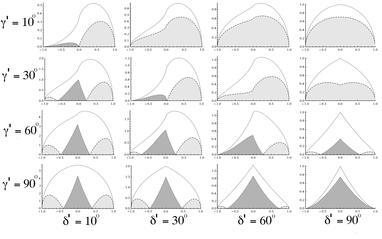
Figure 1: Transverse structure produced by the model considered, for various viewing angles, $\delta^{\prime}$, and helix pitch angles, $\gamma^{\prime}$. Solid lines correspond to total intensity, dark grey regions to longitudinal polarization (EVPAs aligned with the jet) and light grey regions to transverse polarization (EVPAs orthogonal to the jet).

The model described so far describes only the emission mechanism in the rest frame of the jet. If the jet is relativistic then, although the overall levels of flux density will be changed by the Doppler effect and aberration, the transverse profiles will remain unchanged provided that the jet’s velocity is constant across its width.

The Stokes parameters $I$ in the observer’s frame (unprimed) are related to those in the rest frame of the jet (primed) by

$$I(\delta)=I^{\prime}(\delta^{\prime})D^{a}$$ (2.5)

where $\delta$ is the viewing angle in the observer’s frame, $\delta^{\prime}$ is the viewing angle in the rest frame of the jet, $D=[\Gamma(1-\beta\cos\delta)]^{-1}$ is the Doppler factor ($\Gamma$ is the Lorentz factor and $\beta$ the jet velocity divided by the speed of light) and the value of $a$ is $2+\alpha$, where $\alpha$ is the spectral index (Scheuer and Readhead, 1979; Rybicki and Lightman 1979, Chapter 4). Strictly speaking, Equation (2.5) refers to the intensity, $I_{\nu}$, from a continous, optically thin jet, but also applies to the flux density per unit length from a cylindrical jet. The Stokes parameters $Q$ and $U$ transform in precisely the same way.

If the velocity is constant across the width of the cylindrical jet, the Doppler factor is the same for every point in the jet. Therefore, in this case, the Doppler factor will affect only the overall level of the intensity, not the shapes of the $I$, $Q$ or $U$ profiles. More precisely, the jet profiles $I(x)$, $Q(x)$ and $U(x)$ viewed at angle $\delta$ in the observer’s frame will be identical in shape to the profiles $I^{\prime}(x)$, $Q^{\prime}(x)$ and $U^{\prime}(x)$ viewed at angle $\delta^{\prime}$ in the jet rest frame. Because the fits were obtained by comparing only the shapes of the $Q$ and $I$ profiles, without using the absolute intensities of these profiles, the resulting fitted profiles correspond directly to the pitch angle and the viewing angle in the rest frame of the jet. Further, the profiles of the polarization angle and the fractional polarization will be identical in the two frames. To be explicit, a prime is used to denote quantities in the rest frame of the jet, and absence of a prime to denote quantities in the rest frame of the observer.

Although the viewing angles in the observer’s frame are likely to be small, of the order of $1/\Gamma$, where $\Gamma$ is the jet Lorentz factor, the rest-frame viewing angles will be much larger, and it is these rest-frame values that we have derived from our profile fits and quote in the text and tables below.

This is essentially the approach taken by Claussen-Brown, Lyutikov and Kharb (2009), except that they use a force-free magnetic field configuration (and a Gaussian jet profile) defined in the jet’s rest frame, whereas a simple helical field threading a uniform jet has been used here. This choice was made because the objective of this work is precisely to look for observational signatures of a helical field component, rather than to look for additional features that will inevitably be present in more sophisticated models. (Note that Claussen-Brown et al. (2009) quote observer-frame viewing angles, but these can only be given in terms of the (unknown) Lorentz factor.)

Zakamska, Begelman and Blandford (2008) consider a relativistic MHD jet with a toroidal magnetic field. The main difference between this model and Laing’s is the existence of a poloidal field component in Laing’s. A purely toroidal field configuration can give rise to ‘spine–sheath’ polarization structure and systematic transverse Faraday-rotation gradients, but not to asymmetric transverse intensity and polarization structure; therefore, it is of interest to try to investigate such asymmetric structures using the model presented here.

Broderick and Loeb (2009) and Broderick and McKinney (2010) consider theoretical simulations of transverse Faraday rotation measure gradients produced by helical jet magnetic fields. The latter simulations, in particular, directly demonstrate the generation of a helical field and associated Faraday-rotation gradients due to the combination of the rotation of the jet base and the jet outflow. These fully relativistic simulations show that the resulting transverse Faraday-rotation gradients can sometimes prove to be more complex than is predicted by simple helical-field models; however, their origin remains the toroidal component of an essentially helical jet magnetic field.

While detailed models for relativistic jets and their magnetic fields have been investigated in these and other studies, the least model-dependent way to seek evidence for a helical field component is to is to use results for a purely helical field; this amounts to focusing on the basic features of transverse jet profiles rather than aiming to describe them in detail in the face of many unknown parameters. If high-quality, high-resolution data become available for jet profiles, then it may become feasible to investigate more detailed models.

3 Model Predictions

For convenience, the most notable features predicted by this model (Laing 1981), visible in the sample grid of profiles of total and polarized intensity for a range of $\gamma^{\prime}$ and $\delta^{\prime}$ values given in Fig. 1, are summarised here.

1. Except for purely toroidal magnetic fields ($\gamma^{\prime}=90^{\circ}$) or viewing angles (in the rest frame of the jet) perpendicular to the cylinder axis ($\delta^{\prime}=90^{\circ}$), the distributions of total and polarized intensity are usually asymmetric. These asymmetries arise because the change in the sky-projected magnetic-field direction occurs most rapidly along the helical field line on the side of the jet where the angle between the field and the line of sight is smallest. This results in a greater level of polarization cancellation along the line of sight on one side of the jet than the other. The profile asymmetries are clearly seen in cases where neither the helical pitch angle nor the viewing angle equals 90^∘ in Fig. 1.

2. Displacements between the total intensity profile maxima and polarized intensity profile maxima are common.

3. The fractional polarization varies considerably across the profile.

4. The polarized intensity distribution can have one, two or three local maxima, and the orientation of the projected magnetic field can be either longitudinal, transverse or a combination of both within a given profile.

Further examination of the polarization profiles produced by this model shows that 4 different magnetic field distributions are possible, as can be seen in Fig. 1.

1. Longitudinal all across the jet; e.g., $\gamma^{\prime}=10^{\circ}$ and $\delta^{\prime}=30^{\circ}$

2. Longitudinal on one side and transverse on the other; e.g., $\gamma^{\prime}=30^{\circ}$ and $\delta^{\prime}=30^{\circ}$

3. Longitudinal at the edges and transverse at the centre; e.g., $\gamma^{\prime}=30^{\circ}$ and $\delta^{\prime}=10^{\circ}$

4. Transverse all across; e.g., $\gamma^{\prime}=90^{\circ}$ and $\delta^{\prime}=90^{\circ}$

Configuration 2 only occurs when $\gamma^{\prime}=\delta^{\prime}$ and configuration 4 only occurs when $\gamma^{\prime}=\delta^{\prime}=90^{\circ}$. These special cases would not often be expected in nature. However, the effects of finite resolution, in which the true jet profile is convolved with a Gaussian beam, increase the range of parameter values for which configurations 2 and 4 are observed [See Figure 2, adapted from Papageorgiou (2005)].

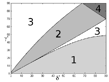
Figure 2: Effect of finite resolution on the observed magnetic field configurations. Convolution was performed using a Gaussian beam with a FWHM one quarter the size of the intrinsic jet width. Region numbers correspond to the configuration types listed in Section 3.

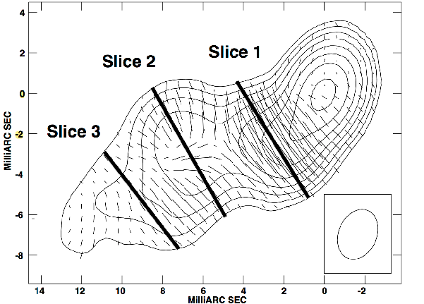
Figure 3: 6cm Polarization Map of Mrk501 for February 1997 (Pushkarev et al. 2005). The polarization sticks are proportional to the polarized intensity. The three lines across the jet show the transverse slices that were analysed. The peak intensity is 0.52 Jy/beam, and the contour levels are 0.60, 1.25, 2.5, 5.0, 10.0, 20.0, 40.0, and 80.0% of the peak.

4 Comparison Method

Table 1: Best fit Parameters for 6cm Mrk501 Slices (Epoch February 1997)

Slices	$\gamma^{\prime}$	$\delta^{\prime}$	$f$	Intrinsic Jet Width
Slice 1	$41^{\circ}\pm 3^{\circ}$	$81^{\circ}\pm 3^{\circ}$	$0.70\pm 0.05$	3.1 mas
Slice 2	$53^{\circ}\pm 1^{\circ}$	$80^{\circ}\pm 2^{\circ}$	$0.40\pm 0.05$	5.7 mas
Slice 3	$47^{\circ}\pm 1^{\circ}$	$90^{\circ}\pm 2^{\circ}$	$0.00\pm 0.10$	4.8 mas

Papageorgiou (2005) did not carry out any formal model fitting, and matched the observed and model profiles using a number of simple criteria. This approach was time consuming, and did not necessarily result in the best fit in a ‘least-squares’ sense. This technique has been improved upon here by generating a database of theoretical profiles to enable a quantitative comparison of the observed and model profiles. To generate such a database an estimate of the intrinsic jet width must first be made. This was done by generating a series of jet profiles of increasing width, which were then convolved with the observing beam. The intrinsic jet width was then taken to be that for which the convolved $I$ profile best matched that observed. Both Gaussian and top-hat model profiles produced similar results. Since the jet width determined in this way is only an estimate, several trial values were used, as is described in Section 5.

The model transverse profiles were generated for a jet with angular width determined as described above and convolved with a Gaussian beam corresponding to the observing beam, varying the values of $\delta^{\prime}$, $\gamma^{\prime}$ and $f$. The best-fit model was taken to be the model giving the smallest residual $\chi^{2}$ between the observed and theoretical profiles:

$$\chi^{2}=\frac{Q_{max}}{I_{max}}\displaystyle\sum\limits_{n=1}^{N}\frac{(I_{n}-I_{n}^{0})^{2}}{\sigma_{I}^{2}}+\displaystyle\sum\limits_{n=1}^{N}\frac{(Q_{n}-Q_{n}^{0})^{2}}{\sigma_{Q}^{2}}$$ (4.1)

where $N$ is the total number of data points, $I_{n}$ and $Q_{n}$ are the $n$th observed total and polarized intensity datapoints respectively, $I_{n}^{0}$ and $Q_{n}^{0}$ are the the $n$th model total and polarized intensity model values respectively, and $I_{max}$ and $Q_{max}$ are the maximum values of the observed total and polarized intensity respectively. The $I$ profiles are downweighted compared to the $Q$ profiles by the factor $Q_{max}/I_{max}$. This factor is close to 0.10 for most of the profiles, and effectively gives the $Q$ and $I$ profiles comparable weights in the fitting, while also ensuring that the polarization structure of the best fit matches the observed polarization structure. In effect, we are ignoring the higher signal-to-noise ratios of the $I$ data, which is justifiable because the real errors that dominate the $I$ image are not due to noise, but instead to mapping errors associated with CLEAN, and there is no reason to believe these should be much smaller than those for $Q$. The results of the fitting do not depend critically on the specific value of this weighting factor. The values of $\sigma_{I}$ and $\sigma_{Q}$ are given by the formulas recently proposed by Hovatta et al. (2012), which are based on Monte Carlo simulations, and include contributions associated with thermal noise and with uncertainty introduced by the CLEAN process; the contribution of residual D-term uncertainty to $\sigma_{Q}$ is negligible for our case, far from the total intensity peak. The thermal-noise component was determined in regions far from the region of source emission.

As the number density of electrons and the magnetic field strength along the slice are unknown, the database profiles were scaled so that the maximum total intensities of the observed and model profiles are equal. Matching the total flux densities of the observed and calculated $I$ profiles would be more accurate; however, doing this would drastically increase the computational time required to complete the comparisons, as each theoretical profile would have to be numerically integrated. In addition, convolution with a beam to mimic the effects of finite resolution removes most of the asymmetries in the theoretical $I$ profiles. As a result, most of the observed $I$ profiles are roughly Gaussian in shape. Thus, the scaling factors corresponding to matching the observed and theoretical profile maxima or the observed and theoretical total fluxes are very similar, justifying our approach.

It is not possible to reliably apply standard statistical approaches to estimating the uncertainties in the resulting parameters without having well determined uncertainties in the fitted quantities — $\sigma_{I}$ and $\sigma_{Q}$. Unfortunately, estimation of the uncertainties associated with values in individual pixels of the $I$ and $Q$ images is not straightforward, since the imaging process is complex and the values in neighbouring pixels will be correlated, due to convolution with the CLEAN beam. Our $\sigma_{I}$ and $\sigma_{Q}$ estimates should typically correspond to uncertainties in individual pixels that are correct to within a factor of a few; nevertheless, these estimates may not be good enough to yield fully accurate $\chi^{2}$ values. Therefore, although the calculated $\chi^{2}$ values can certainly be used to compare the profiles correspond to yielded by different sets of model parameters and identify a set of parameters yielding a best fit, the $\chi^{2}$ values cannot be used to evaluate the overall goodness of the fits obtained; an alternative method used to obtain estimates of the uncertainties in the fitted parameters in Section 5 is described below.

This method was applied to profiles for slices along which the EVPA was either parallel or perpendicular to the jet direction. The Stokes parameters $Q$ and $U$ are defined such that $Q$ is positive and $U=0$ when the EVPA is parallel to the jet.

5 Markarian 501 (Mrk 501)

Table 2: Best fit Parameters for Mrk 501 Slice 2 at 3 different wavelengths

Wavelength	$\gamma^{\prime}$	$\delta^{\prime}$	$f$	Epoch	Intrinsic Jet Width
4 cm	$53^{\circ}\pm 1^{\circ}$	$83^{\circ}\pm 2^{\circ}$	$0.40\pm 0.20$	February 1997	5.5 mas
6 cm	$53^{\circ}\pm 1^{\circ}$	$80^{\circ}\pm 2^{\circ}$	$0.40\pm 0.05$	February 1997	5.7 mas
13 cm	$54^{\circ}\pm 1^{\circ}$	$86^{\circ}\pm 2^{\circ}$	$0.35\pm 0.05$	May 1998	21.6 mas
18 cm	$54^{\circ}\pm 1^{\circ}$	$81^{\circ}\pm 2^{\circ}$	$0.60\pm 0.05$	May 1998	22.9 mas

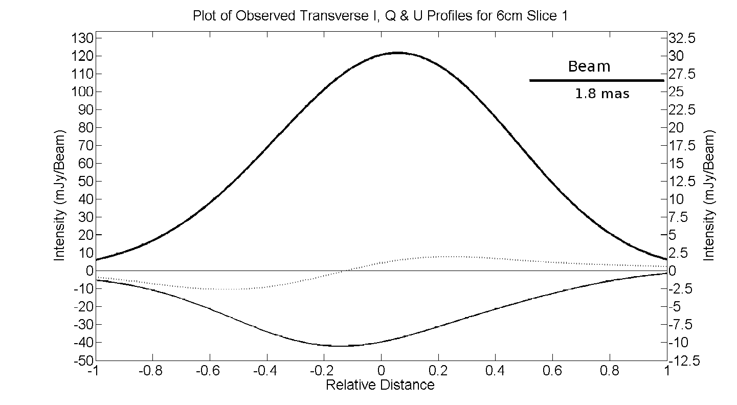
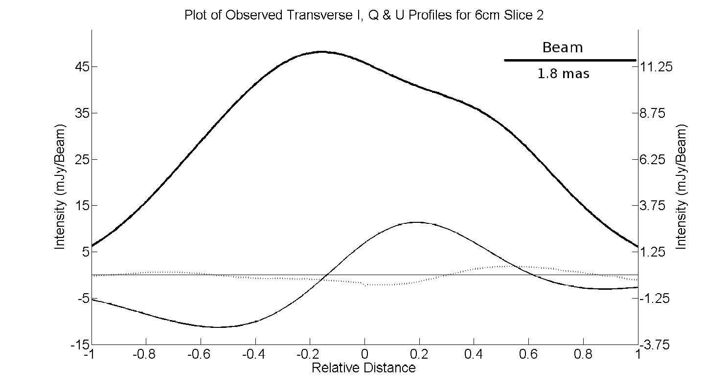
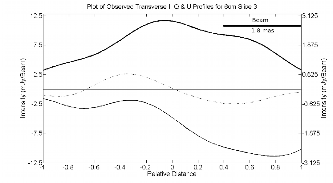
Figure 4: Observed $I$ (solid), $Q$ (dashed) and $U$ (dotted) profiles for Slices 1, 2 and 3 (top to bottom) of the 6 cm Mrk501 map (see Fig. 3). The scale for the $I$ profile is given along the left-hand vertical axis and the scale for the $Q$ and $U$ profiles along the right-hand vertical axis. The beam is 1.8 mas along the slice and 2.4 mas transverse to the slice.

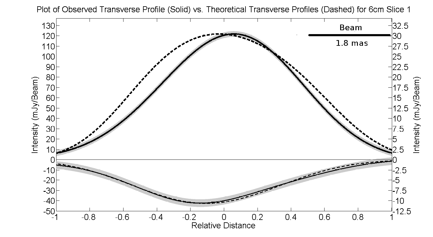
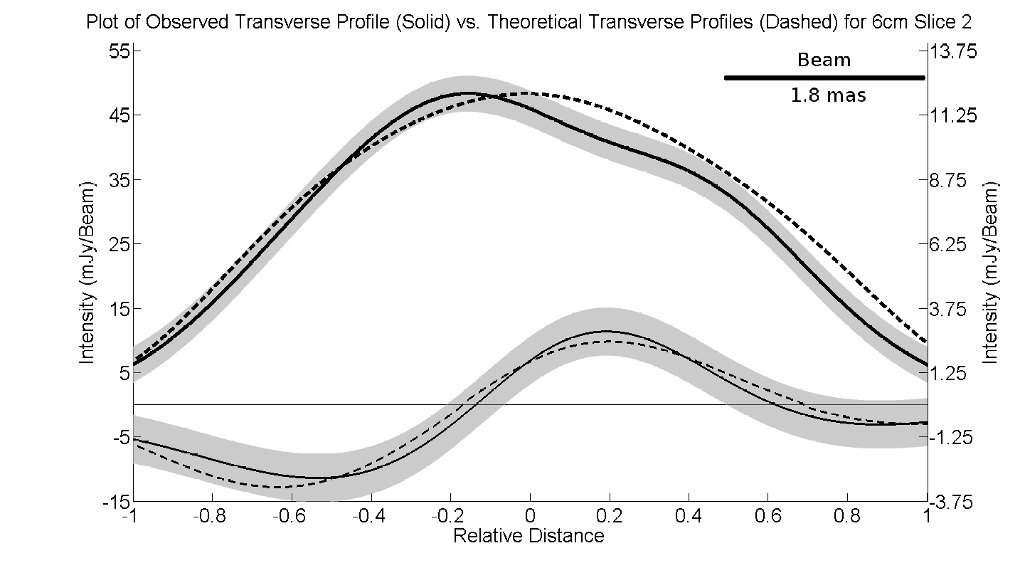
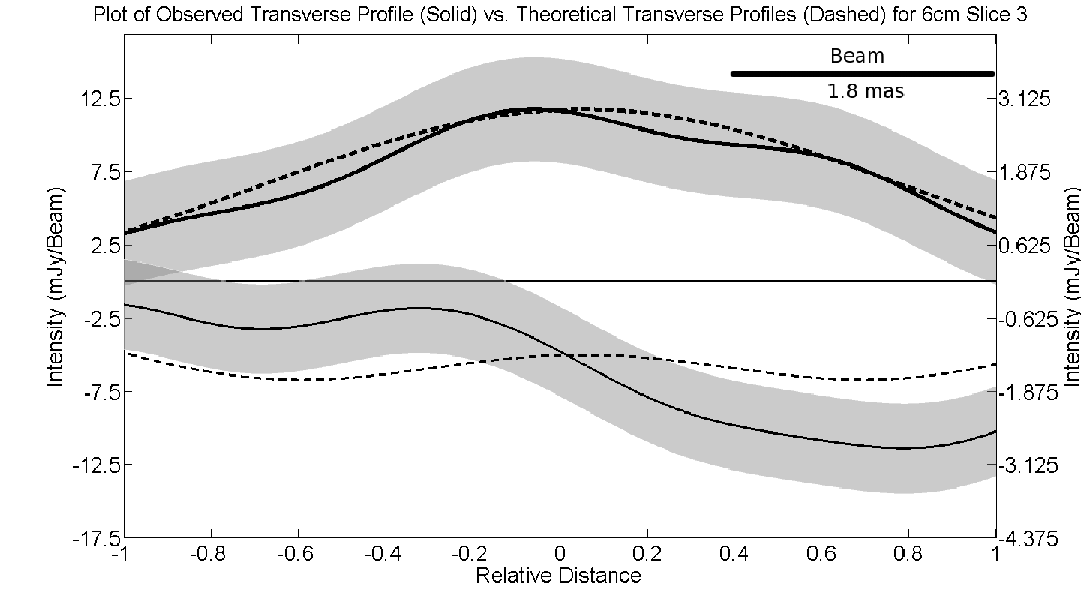
Figure 5: Plots of observed and best-fit model $I$ and $Q$ profiles for Slices 1, 2 and 3 (top to bottom) of the 6 cm Mrk501 map (see Fig. 3). The observed profiles are solid and the best-fit profiles dashed; the gray shaded areas surrounding the observed profiles correspond to the range of the $1\sigma$ uncertainties for $Q$ and the $3\sigma$ uncertainties for $I$. The scale for the $I$ profile is given along the left-hand vertical axis and the scale for the $Q$ profile along the right-hand vertical axis. The beam is 1.8 mas along the slice and 2.4 mas transverse to the slice.

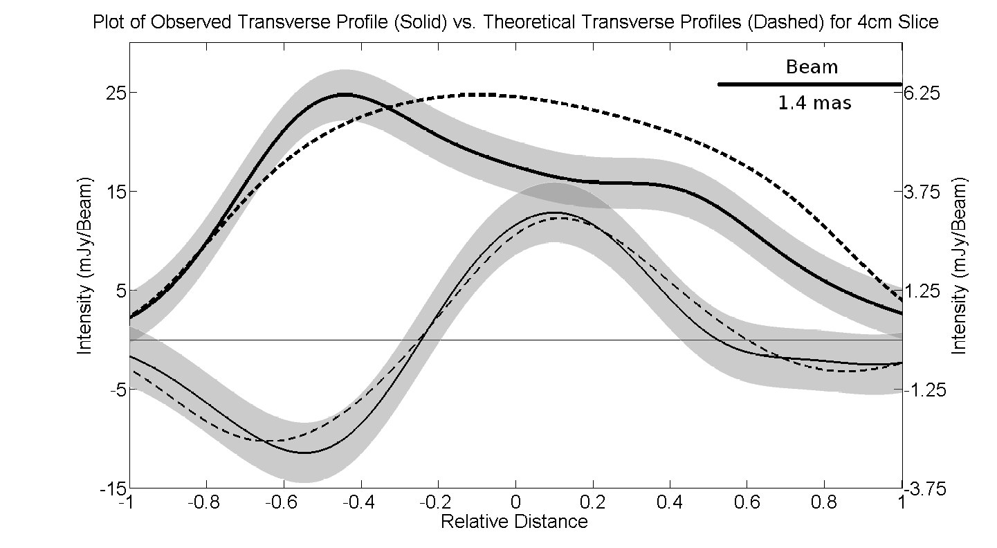
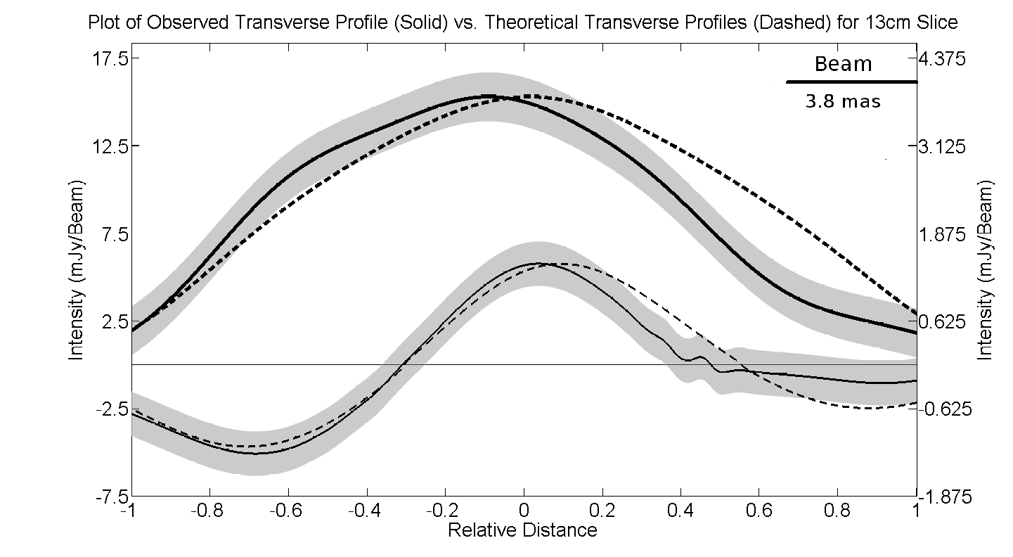
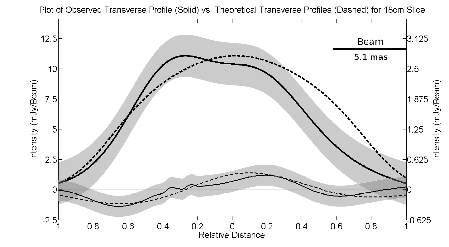
Figure 6: Plots of observed and best-fit model $I$ and $Q$ profiles for 4 cm (top), 13 cm (middle) and 18 cm (bottom) slices taken in the same region as Slice 2 (see Fig. 3). The observed profiles are solid and the best-fit profiles dashed; the gray shaded areas surrounding the observed profiles correspond to the range of the $1\sigma$ uncertainties for $Q$ and the $3\sigma$ uncertainties for $I$. The scale for the $I$ profile is given along the left-hand vertical axis and the scale for the $Q$ profile along the right-hand vertical axis. The beam sizes along and transverse to the slice are 1.4 mas and 1.6 mas (4 cm), 3.8 mas and 2.8 mas (13 cm) and 5.1 mas and 3.8 mas (18 cm), respectively.

An ideal VLBI jet for an analysis based on the method described in Section 4 would be one that is straight, well resolved and shows clearly visible transverse $I$ and $Q$ structure, with $U$ small compared to $Q$. Well-resolved VLBI jets are rare, however, and most VLBI jets contain some bends (though many of these are most likely small bends amplified by projection). Thus, VLBI jets displaying clear transverse structure, especially in polarization, were sought, with the aim of determining whether profiles across such jets could plausibly be represented using the helical field model outlined in Section 2. This requires measuring these profiles away from bends, along directions orthogonal to the local jet direction.

The well known active galaxy Mrk 501 (1652+398), which has been classified as a BL Lac object with redshift $0.034$ (de Vaucouleurs et al, 1991), has been chosen for this initial study. The jet of Mrk 501 is almost certainly relativistic, as is shown by its one-sidedness; however, the shapes of the observed jet intensity and polarization profiles should be unaffected by this relativistic motion. Piner et al. (2010) have found apparent component speeds significantly less than the speed of light in the Mrk 501 jet. At first sight, this would suggest a non-relativistic jet, at variance with the one-sidedness of the jet (unless the VLBI jet were intrinsically one-sided). In the context of the standard model for VLBI jets, it seems far more likely that these low component speeds represent either relativistic motion at a very small angle to the line of sight or pattern speeds that do not directly reflect the speeds of the emitting plasma. In fact, a possible detection of superluminal motion with $v=(3.3\pm 0.3)c$ based on 43 and 86-GHz VLBI images has been reported for this source (Piner et al. 2009). The most detailed multi-wavelength studies of Mrk 501 have been carried out by Giroletti et al. (2004, 2008). They derived constraints on the intrinsic speed of the jet $\beta$ and angle of the jet to the line of sight in the observer’s frame $\delta$ on various scales, finding $\delta\leq 27^{\circ}$ and $\beta\geq 0.88$, but with high values $\beta>0.95$ allowed only for $10^{\circ}<\delta<27^{\circ}$. They also found evidence for limb brightening in total intensity on somewhat larger scales than those studied here, which they attributed to transverse velocity structure of the jet. In particular, they proposed that the jet has a a fast spine and a slower sheath, as suggested by Laing (1996), with the two experiencing different degrees of Doppler boosting. The observed limb brightening could also have other origins, such as an enhancement in the synchrotron emission coefficient at the edges of the jet due to interaction of outer layers of the jet with the surrounding medium, or a helical magnetic field confined to a thin shell (e.g. Laing 1981).

Our selection of Mrk 501 for our analyses is motivated by the fact that VLBI images of this AGN show a variety of transverse structures that could potentially be associated with a helical jet magnetic field, most notably a fairly clear ‘spine–sheath’ polarization structure, corresponding to configuration 3 of Fig. 2 (e.g. Pushkarev et al. 2005). In addition, being at a relatively low redshift, the VLBI jet of Mrk 501 is relatively well resolved, compared to VLBI jets in more distant AGNs.

Fig. 3 shows a 6 cm total intensity map of this source with the polarization position-angle sticks superimposed, constructed from the same data as those of Pushkarev et al. (2005), from February 1997. Near the core, the EVPAs are predominantly perpendicular to the jet direction, maintaining this orientation as the jet direction begins to change about 6 mas from the core. Beyond this region, the EVPAs are perpendicular to the jet near the two edges and parallel in the centre, forming the spine–sheath polarization structure referred to above. The observational results of Giroletti et al. (2004, 2008) on comparable scales to those studied here are broadly similar to those presented in Fig. 3, though at higher resolution, so that the transverse asymmetry is more apparent.

The choice of distances along the jet at which to analyse the transverse profiles is constrained by the need to find places where the EVPAs are either parallel or perpendicular to the jet (i.e., where $U$ is close to close to zero all across the jet), and the $Q$ profiles have sufficiently high signal-to-noise. The profiles to be analyzed were constructed at locations where these conditions are satisfied, far from positions where the jet bends. A further constraint on choice of position arises due to the fact that the jet is essentially unresolved in the immediate vicinity of the core.

The three 6 cm slices chosen for analysis are marked on Fig. 3. The profiles were sampled using the AIPS task ‘SLICE’, then compared to the database of model profiles (each convolved with the Gaussian observing beam) as described in Section 4, and the values of $\gamma^{\prime}$, $\delta^{\prime}$ and $f$ resulting in the best fit (minimum residual) identified (given in Table 1). The intervals between adjacent values of $\gamma^{\prime}$, $\delta^{\prime}$ and $f$ in the database were $1^{\circ}$, $1^{\circ}$ and $0.05$, respectively.

The observed $I$ (solid), $Q$ (dashed) and $U$ (dotted) profiles for the three 6 cm slices are shown in Fig. 4. The left and right sides of the horizontal axis in this figure correspond to the North and South sides of the Mrk 501 jet. Recall that the Stokes parameters are defined such that $Q$ is positive and $U$ is zero for a polarization $E$ field parallel to the jet. $U$ must be small (much less than $Q$) for the model used to be valid; the plots show that this condition is satisfied for the three slices chosen.

The observed (solid) and best-fit model (dashed) profiles $I$ and $Q$ for the three slices are shown in Fig. 5. Here also, the left and right sides of the horizontal axis correspond to the North and South sides of the Mrk 501 jet. The $I$ and $Q$ curves in Fig. 5 are easily distinguishable, as the $Q$ curves are much smaller in amplitude; the intensity scale for $I$ is shown to the left and that for $Q$ to the right. The shaded bands around the $I$ and $Q$ profiles in Fig. 5 correspond to $3\sigma$ and $1\sigma$ uncertainties respectively, estimated in accordance with the approach of Hovatta et al. (2012). Unconstrained fits for slice 3 yielded best-fit parameters corresponding to an opposite sense of the helicity of the magnetic field, compared to slices 1 and 2; this corresponds to the fact that $Q$ changes from negative to positive across slice 2, but becomes more negative across slice 3 (Fig. 4). Since such a change in helicity between slices 2 and 3 is physically implausible, we obtained fits to slice 3 constraining the sense of the helicity of the magnetic field to be the same as for slices 1 and 2; this is the fit shown in Fig. 5 (and given in Table 1). The best-fit model $Q$ profiles for slices 1 and 2 lie within $1\sigma$ of the observed $Q$ profile, while the best-fit $Q$ profile for slice 3 lies within $2\sigma$ of the observed profile. The model and observed $I$ profiles for slices 1 and 2 differ by more than $3\sigma$ over sustantial fractions of these profiles, with the model profile being more symmetrical than the observed profile; the fitted and observed $I$ profiles for slice 3 agree to within about $2\sigma$.

Since the intrinsic (or unconvolved) angular jet width was estimated using the procedure outlined in Section 4, the fitting procedure was repeated for a series of intrinsic jet widths centered on the values used above and listed in Table 1. Changing the intrinsic jet width had only a very minor effect on the best fit $\gamma^{\prime}$ and $\delta^{\prime}$ values while having a more pronounced effect on the degree of entanglement. However, in general, as the intrinsic jet width varied from its estimated value, the $\chi^{2}$ value of the best fit profiles increased. While the intrinsic jet width that minimised the $\chi^{2}$ value for a given slice is not exactly that found by fitting the $I$ profile, the two never differed by more then $10\%$. Values differing by more than $15\%$ yielded very large values of $\chi^{2}$.

As was noted above, the uncertainties in the fitted parameters cannot be estimated reliably using standard statistical techniques, since the values of $\sigma_{I}$ and $\sigma_{Q}$ used are only estimated uncertainties. Instead, estimates of the parameter uncertainties were derived by carrying out Monte Carlo simulations, as follows. Infinite resolution model maps corresponding to model parameters corresponding to those inferred for the Mrk501 jet were generated, and the Fourier transforms of these maps sampled at the set of baselines corresponding to the observations. This effectively yielded model visibilities at the set of UV baselines that were actually observed. Noise consistent with the noise levels observed in the images was then added. The resulting ‘noisy’ model data were imaged in AIPS in the usual way, profiles were taken across the resulting maps and these profiles were subject to the same fitting process as the real observed profiles. The resulting best-fit parameters were then compared to the parameters used to generate the model maps to estimate the uncertainty in the fitting process. This was carried out for 200 Monte Carlo realizations of the model data, and the distribution of derived uncertainties used to estimate the corresponding $1\sigma$ uncertainties, listed in Tables 1 and 2.

The line-of-sight angles, $\delta^{\prime}$, for the first two slices in Table 1 agree to within a degree, and differ by less than $1\sigma$, as expected if the intrinsic bends in this region of the jet are small. The value of $\delta^{\prime}$ for slice 3 differs by about $10^{\circ}$ ($\delta^{\prime}=90^{\circ}$), which corresponds to about $3.5\sigma$; however, as was pointed out above, it was necessary to constrain the fit for slice 3 to have the same sense of helicity as slices 1 and 2. Therefore, we do not feel confident that the change in viewing angle implied by the nominal (constrained) best fit for slice 3 is significant.

The fitting results indicate a somewhat higher value of $\gamma^{\prime}$ for slice 2 than for slice 1, with this difference being about $4\sigma$, suggesting that the variation in $\gamma^{\prime}$ between the slices may be real. In this case, this suggests that the appearance of a spine–sheath polarization structure at the position of slice 2 could be due to a (relatively small) change in the helical pitch angle. The value of $\gamma^{\prime}$ for slice 3 lies between the values for the other two slices; formally, $\gamma^{\prime}$ for slice 3 differs from the value for slice 2 by about $3.5\sigma$, and from the value for slice 1 by slightly less than $2\sigma$.

The values of $f$ appear to decline with distance from the core, from $0.7$ at slice 1 to $0.4$ at slice 2. This trend may continue for slice 3 ($f=0$), although this is unclear due to the uncertainty associated with slice 3 discussed above. The difference between slices 1 and 2 appears to be significant: the two $f$ values differ by approximately $4\sigma$; physically, this represents a decrease in the disordered component of the magnetic field with distance from the core in the region of the jet sampled.

The fitting procedure was repeated for slice 2 using images at wavelengths of 4 cm for February 1997 (data of Pushkarev et al. 2005) and $13$ cm and 18 cm for May 1998 (data of Croke et al. 2010). The results are given in Table 2 and shown in Fig. 6. It is clear that the observations at these other wavelengths yield consistent best-fit parameter values; the values of $\gamma^{\prime}$, $\delta^{\prime}$ and $f$ essentially all agree to within $1\sigma$, with the largest differences not exceeding about $2\sigma$.

Fits were also obtained for Slices 1, 2 and 3 using Model B of Laing (1981), which consists of a cylinder of fixed radius containing a randomly orientated magnetic field with no radial component. The only parameter in this model is the viewing angle. This model can produce a region of transverse field at the jet axis surrounded by regions of longitudinal field, but the profiles produced by this model are completely symmetric. Because Model B also produced profiles that are considerably more strongly polarized than is observed, we included the degree of entanglement $f$ in these models as well. Figure 7 shows the best-fit profiles for the three slices for the 6cm image of Mrk501. The model fits for slices 1 and 2 are clearly considerably poorer than those in Fig. 5. In contrast to Fig. 5, where the model and observed $Q$ profiles agree to within $1\sigma$ everywhere, the differences between the model and observed $Q$ profiles in Fig. 7 exceed $1\sigma$ essentially everywhere, with the differences exceeding $3\sigma$ along most of the profiles. The fit for Model B for slice 3 is very similar to the corresponding fit for the helical-field model in Fig. 5. Thus, while Model B of Laing (1981) can provide a comparably good fit for slice 3, it does not provide a viable alternative to the polarization structure across the other two slices.

6 Spectral Index

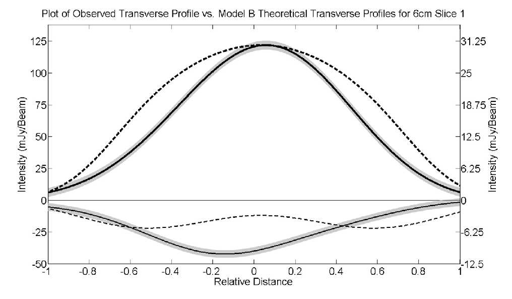
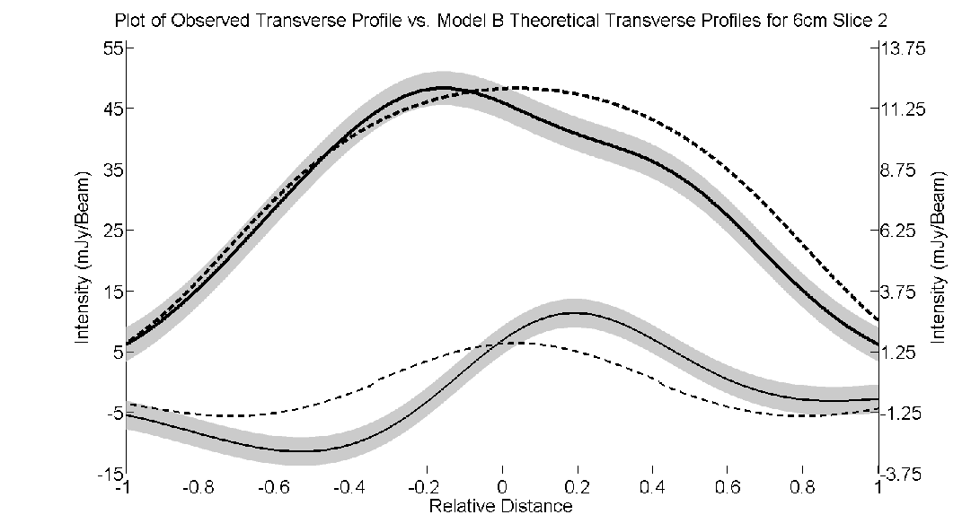
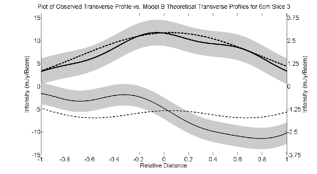
Figure 7: Plots of observed and best-fit model $I$ and $Q$ profiles for 6 cm slices 1, 2 and 3 obtained for Model B of Laing (1981). The observed profiles are solid and the best-fit profiles dashed; the gray shaded areas surrounding the observed profiles correspond to the range of the $1\sigma$ uncertainties for $Q$ and the $3\sigma$ uncertainties for $I$. The scale for the $I$ profile is given along the left-hand vertical axis and the scale for the $Q$ profile along the right-hand vertical axis. The beam is 1.8 mas along the slice and 2.4 mas transverse to the slice.

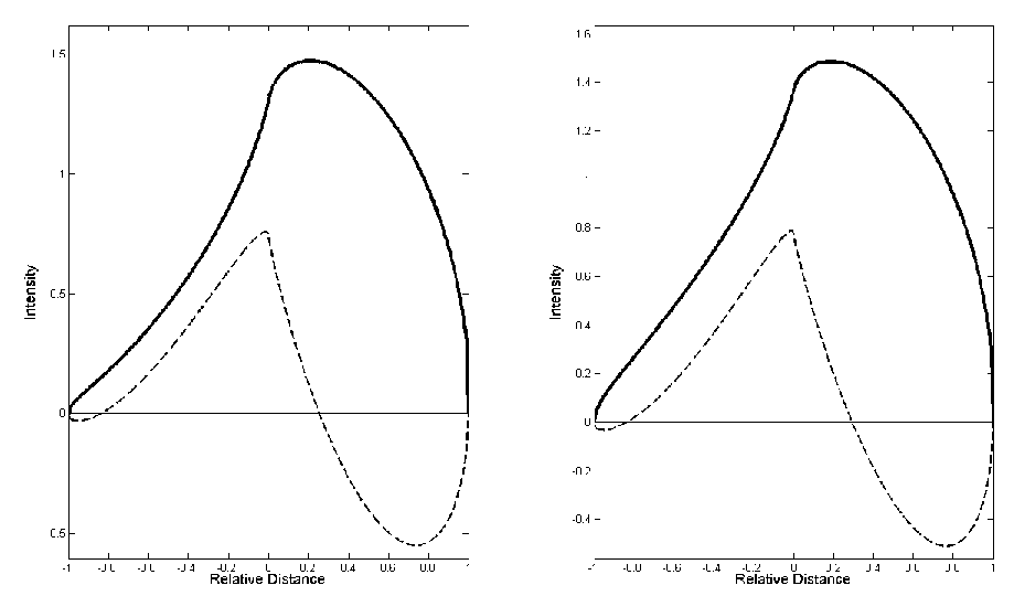
Figure 8: Theoretical profiles generated numerically for $\gamma^{\prime}=60^{\circ}$, $\delta^{\prime}=40^{\circ}$ and $f=0$. The left and right profiles were determined for $\alpha=1.0$ and $\alpha=0.5$, respectively. The magnetic-field orientation is perpendicular to the polarization orientation.

A spectral index ($\alpha$) of unity was assumed throughout the jet in order to make the equations that govern this model analytically solvable. However, observations of the spectral indices in the jets of AGN have shown that this value is typically $\simeq 0.5$. This gives rise to concerns about the trustworthiness of the fits obtained assuming $\alpha=1.0$. To investigate this, model profiles were obtained numerically for two other spectral indices.

Profiles for both $I$ and $Q$ were determined numerically by integrating equations A1 and A2 from Laing (1981) using the Gauss-Kronrod quadrature (Kronrod, A.S., 1964). This method was required as the functions governing both $I$ and $Q$ have singularities at one of their limits.

Figure 8 shows the effect of variations in the spectral index on the $I$ and $Q$ profiles. The left and right hand plots show profiles for jets with $\alpha=1$ and $\alpha=0.5$ respectively, and the same values of $\gamma$, $\delta$ and $f$. The differences between these profiles are very small. The positions where the polarization angle changes by 90^∘ are slightly different. In addition, the amount of longitudinal polarization has increased slightly, while the amount of transverse polarization has decreased. This second difference results in the configuration map for $\alpha=0.5$ being slightly different to that for $\alpha=1$ (compare Fig. 2 and 9).

The effect of changing spectral index on the best fit model values of $\gamma^{\prime}$, $\delta^{\prime}$ and $f$ was examined using slices through the 13 cm images at the location of Slice 2 in Fig. 3. Model databases were then generated numerically using values of $\alpha=0.507$ (the average value of $\alpha$ across the slice) and $\alpha=0.248$ (the minimum value of alpha across the slice, representing the maximum deviation from unity) and the FWHM of the beam used in creating the 13 cm map. These databases were then used to obtain new best-fit parameters for the 13 cm slice. The results are shown in Table 3. The differences in the best fit parameters are extremely small with the $\gamma^{\prime},\delta^{\prime}$ and $f$ values for the two numerically calculated best-fit profiles ($\alpha=.508$ and $\alpha=.248$) and the analytically calculated best-fit profile (for $\alpha=1.0$) all coinciding within the 1$\sigma$ errors.

Table 3: Best fit Parameters for 13 cm Mrk501 Slice for three values of $\alpha$

$\alpha$	$\gamma^{\prime}$	$\delta^{\prime}$	$f$
1.000	$54^{\circ}\pm 1^{\circ}$	$86^{\circ}\pm 2^{\circ}$	$0.35\pm 0.05$
0.507	$53^{\circ}\pm 3^{\circ}$	$85^{\circ}\pm 2^{\circ}$	$0.40\pm 0.05$
0.248	$53^{\circ}\pm 1^{\circ}$	$84^{\circ}\pm 2^{\circ}$	$0.40\pm 0.05$

7 Comparison with Results from Faraday Rotation profiles

As described earlier, the fractional polarization from the helical field model is generally lower on the side of the jet where the field lines are closest to the line of sight. If the magnetic field threading the Faraday rotating medium is comoving with the jet and is threaded by the same magnetic field, the magnitude of the Faraday rotation measure will be highest on the side of the jet where the field lines are closest to the line of sight, i.e., on the side with the lower fractional polarization. It is therefore of interest to check whether the transverse polarization and Faraday-rotation profiles observed for the Mrk 501 jet are consistent with this picture. In particular, Gabuzda et al. (2004) reported the detection of a transverse Faraday rotation measure (RM) gradient across the Mrk 501 jet, based on 2+4+6 cm VLBA polarization observations, and interpreted this as evidence for a helical magnetic field associated with this jet. Croke et al. (2010) subsequently reported a transverse RM gradient in the same sense based on 4+6+13+18 cm VLBA polarization observations.

Taylor & Zavala (2010) have recently questioned the validity of reported transverse RM gradients, and proposed a number of criteria for the reliable detection of such gradients, namely that there be (i) at least three “resolution elements” (taken to mean three beamwidths) across the jet, (ii) a change in the RM of at least three times the typical error $\sigma$, (iii) an optically thin synchrotron spectrum at the location of the gradient, and (iv) a monotonic, smooth (within the errors) change in the RM from side to side. The more recent Monte Carlo simulations of Hovatta et al. (2012) suggest that a more reasonable limit for the distance spanned by the RM values comprising the gradient is two beamwidths if the RM values differ by at least $3\sigma$, and as little as 1.5 beamwidths in the case of higher signal-to-noise ratios.

As part of their study, Taylor & Zavala (2010) consider several RM maps based on multi-wavelength 2–4 cm VLBA data, searching for RM gradients specifically in regions where the RM distributions span more than three beamwidths. On this basis, they report an absence of significant transverse RM gradients in the Mrk 501 jet, based on profiles taken roughly 10 mas from the core, and therefore call into question the earlier results of Gabuzda et al. (2004) and Croke et al. (2010). We do not wish to analyze this discrepancy between the results of Gabuzda et al. (2004) and Croke et al. (2010), on the one hand, and Taylor & Zavala (2010), on the other hand, in full detail here. However, for transparency, we will make some remarks concerning this, as a justification for our further consideration of the results of Gabuzda et al. (2004) below.

The transverse RM gradient reported by Gabuzda et al. (2004) essentially satisfies the last three criteria of Taylor & Zavala (2010), but not the first; however, because the gradient spans approximately 1.7 beamwidths, it marginally satisfies the modified criterion of Hovatta et al. (2012). The gradient reported by Croke et al. (2010) spans roughly four beamwidths across the jet, and satisfies all four criteria of Taylor & Zavala (2010). Note that the profile considered by Taylor & Zavala (2010) is further from the core than the region considered by Gabuzda et al. (2004), where the magnitude of the RM values would be expected to be lower; the region considered by Croke et al. (2010) overlaps with the region of the profile of Taylor & Zavala (2010), but the data of the former study were considerably more sensitive to small amounts of Faraday rotation, since they included observations at the longer wavelengths of 13 and 18 cm.

Thus, while the resolution of the images of Gabuzda et al. (2004), analyzed in the same general region as our own profiles, may not represent conclusive proof of a uniform transverse RM gradient, their results can reasonably be considered at least tentative evidence for a Faraday-rotation gradient across the Mrk 501 jet, particularly in light of the subsequent, better-resolved results of Croke et al. (2010). Therefore, we feel justified in using these results as a working hypothesis. We emphasize that we are interested here only in the very crude question of whether there seems to be a higher typical RM magnitude on one or the other side of the VLBI jet, and whether this is consistent with the side predicted by our simple model.

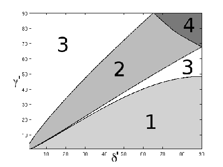
Figure 9: Magnetic-field configuration map analogous to Fig. 2 for $\alpha=0.5$ after convolution with a Gaussian beam with a FWHM one-quarter the size of the profile to mimic the effects of finite resolution. The region numbers correspond to the configuration types listed in Section 3.

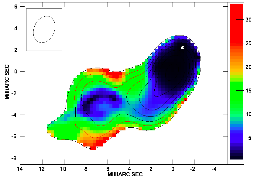
Figure 10: 6 cm total intensity contours given in Fig. 3 superposed with a colour image of the distribution of the degree of polarization. The increase in the degree of polarization toward the edges of the jet, also reported by Pushkarev et al. (2005), is clearly visible. The locations of the highest degrees of polarization do not coincide with those expected for curvature-induced polarization.

In the regions of the jet considered here, comparing the two sides of the jet, the Northern side (corresponding to the left-hand sides of the plots in Figs. 5–6) generally displays higher fractional polarization, i.e., more negative values of $Q/I$. It follows that the Faraday rotation measures on the Northern side of the jet, RM_N, are expected to be smaller in magnitude than those on the Southern side, RM_S. This is consistent with the observational results of Gabuzda et al. (2004), based on the same 2–6 cm VLBA data considered here: $\textrm{RM}_{N}=-55\pm 20$ rad/m², $\textrm{RM}_{S}=130\pm 20$ rad/m². The effect of the measured Galactic rotation measure in the direction toward Mrk 501 [$+42$ rad/m², Rusk (1988)] was subtracted from the observed polarization angles before the Faraday rotation map was constructed, so that the residual observed rotation measure should correspond to Faraday rotation occurring in the vicinity of the AGN. If the Galactic rotation measure is instead taken to be the value typical of the region within a few degrees of Mrk 501 in the catalog of Taylor, Stil and Sunstrum (2009), $\simeq+20$ rad/m², these two values become $\textrm{RM}_{N}\simeq-35$ rad/m², $\textrm{RM}_{S}\simeq 150$ rad/m².

We can crudely estimate the expected quantitative difference between the magnitudes of the Faraday rotation measures on either side of the jet if the Faraday rotating material is concentrated in a relatively thin shell in outer layers of the jet using Eq. (2) of Laing (1981): for $\gamma^{\prime}=40^{\circ}$ and $\delta^{\prime}=80$, this indicates a difference of about 35%, somewhat smaller than the observed value of about $60-75\%$.

Considering this one case, and given the limited transverse resolution of the rotation-measure image of Gabuzda et al. (2004), it could be a coincidence that the model considered correctly predicts the side of the jet that should have the higher Faraday rotation. However, our analysis here illustrates the sort of comparison that could, in principle, usefully be carried out once profile-fitting results for a greater number of AGNs are available. Of course, the sign of the Faraday rotation measures cannot be predicted by our model, as the polarization profiles do not depend on the polarity of the magnetic field.

8 Derivation of $\delta$ and $\beta=v/c$ in the Observer’s Frame

The line of sight angle $\delta^{\prime}$ in the rest frame of the jet is related to the corresponding angle in the observer’s frame, $\delta$, by

$$\sin\delta^{\prime}=\frac{\sin\delta}{\Gamma[1-\beta\cos\delta]}$$ (8.1)

where $\Gamma$ is the Lorentz factor for the motion and $\beta=v/c$ (Rindler 1990).

In addition, the apparent speed of a component moving along the jet can be written

$$\beta_{app} = \frac{\beta\sin\delta}{1-\beta\cos\delta}$$ (8.2)

$$= \Gamma\beta\sin\delta^{\prime}$$ (8.3)

$$= (\beta^{-2}-1)^{-1/2}\sin\delta^{\prime}$$ (8.4)

It follows that, if $\beta_{app}$ is known from component motion and $\delta^{\prime}$ is known, for example, from profile fitting such as that carried out in this paper, Equation (8.4) can be rearranged to give

$$\beta=\left[1+\frac{\sin^{2}\delta^{\prime}}{\beta_{app}^{2}}\right]^{-1/2}$$ (8.6)

The profile fitting has indicated $\delta^{\prime}\simeq 83^{\circ}$ for the Mrk 501 jet. Taking this together with the superluminal motion reported by Piner et al. (2009), $\beta_{app}=3.3$, gives $\beta\simeq 0.96$ and $\delta\simeq 15^{\circ}$. Using the range of $\delta^{\prime}$ values given by the various profile fits, $80^{\circ}-86^{\circ}$, does not change the resulting values of $\delta$ by more than $1^{\circ}$. These results are consistent with the conclusion of Giroletti et al. (2004), based on completely different information, that $\delta\leq 27^{\circ}$ and $\beta\geq 0.88$, with $\beta>0.95$ allowed only for $10^{\circ}<\delta<27^{\circ}$. Although these particular results are somewhat uncertain, since the relevant superluminal motion corresponds to a weak feature whose position is difficult to determine precisely, this illustrates the potential of this approach. Note as well that using the more typical subluminal speeds obtained for the jet of Mrk 501, e.g. $\beta_{app}\simeq 0.47$ (Piner et al. 2010), implies angles to the line of sight $\delta\simeq 60^{\circ}$ and $\beta\simeq\beta_{app}$, which are not reasonable, since they cannot provide the observed one-sided VLBI structure. This implies that the very low component speeds typically observed in Mrk 501 are incompatible with its observed polarization structure, and so must represent pattern speeds rather than physical speeds (in other words, they do not represent highly relativistic motion viewed at a very small angle).

The approach taken in this section is similar to that used by Canvin et al. (2005) on kiloparsec scales, in that both analyses fit a jet model to the observed profile in order to determine the angle between the jet axis and the line of sight in the rest frame of the flow. One advantage of applying this technique on parsec scales is that it is possible to obtain constraints on the underlying flow speed fairly directly using observations of superluminal components, whereas, in the kiloparsec case, more indirect estimate must be used, such as the jet–counterjet brightness ratio.

9 Discussion

In general, the procedure described above has yielded good fits to the polarization data for Mrk 501. The deviations between the model and observed $Q$ values for slices 1 and 2 are less than the estimated $1\sigma$ uncertainties for the observed $Q$ profiles, while the discrepancies for the somewhat uncertain slice 3 are less than $2\sigma$ (Hovatta et al. 2012). The model has thus successfully reproduced the main features of the observed polarization. The total intensity fits were much less successful, with the model profiles generally being appreciably more symmetrical; differences between the observed and model $I$ profiles were within $2\sigma$ for the 6-cm Slice 3, but frequently exceed $3\sigma$ for the other slices considered. Whether this discrepancy between the model and observed $I$ profiles is due to other factors giving rise to asymmetry in the observed $I$ profiles or unsuitability of the model is not clear. For this reason, the results presented here should be considered tentative.

Formally good model fits were not expected using the procedures described in this paper; the main goal was to determine whether a simple helical-field model such as that considered here is able to qualitative reproduce the shapes of the observed profiles, particularly in $Q$. In fact, there are many reasons why it would be unreasonable to expect a formally good fit to both $I$ and $Q$. The structure of the jet may differ in many ways from the simple structure used here. For example, any deviation from perfect cylindrical symmetry, or an emissivity that changes with distance from the jet axis, would introduce features that could not be reproduced by the model. Some such physical deviations may be responsible for the double–peaked $I$ structure in the $3.6$ cm profile in Fig. 6, which is poorly represented by the model. Attempting to introduce further parameters into the model would result in fits that were much more poorly constrained by the data. Given the simplicity of the model used, its ability to reproduce the $Q$ profiles so well is striking.

Thus, the most important result of our profile fitting is that even the simple helical-field model considered here can reproduce most of the qualitative features of the polarization profiles, lending support to the hypothesis that a helical magnetic-field component is present in the jet of Mrk 501 on parsec scales.

9.1 Curvature-Induced Polarization?

Given the observed bends in the jet of Mrk 501, it is natural to ask whether the observed polarization structure is associated with curvature of the jet. As the jet bends, the jet plasma is squeezed and stretched at the inside and outside edges, respectively. If, as seems to be the case here, the magnetic field is highly disordered, but with a mean value of $<B_{long}^{2}>$ greater than $<B_{perp}^{2}>$, where $B_{long}$ and $B_{perp}$ are the magnetic fields along and perpendicular to the jet, then squeezing the plasma along the jet axis will increase $<B_{perp}^{2}>$, reducing the degree of polarization, while stretching the plasma in this same direction will have the opposite effect. This effect would increase/decrease the degree of polarization at the outside/inside edges of jet bends.

To investigate this, we constructed a map of the degree of polarization $m$ at 6 cm, shown in Fig. 10. The observed fractional polarization is greatest at the edges of the jet (reaching values $\simeq 25-30\%$), as is expected for curvature-induced polarization. However, the locations of highest fractional polarization are on the inside edges of local bends in the jet (the northern side of the jet between slices 1 and 2, and the southern side of the jet beyond slice 2), whereas curvature-induced polarization should be highest on the outside edges of these bends. Therefore, we find no evidence that the longitudinal polarization observed at the edges of the Mrk 501 jet is primarily induced by the curvature of the jet as it bends.

10 Conclusions

A method for comparing model and data profiles for total intensity and polarization in astrophysical jets has been described and demonstrated. The method has been used to compare observed profiles of the parsec-scale jet of Mrk 501 with the predictions of a model in which a cylindrical jet is permeated by a magnetic field with a uniform helical component and a disordered component.

The jet of Mrk 501 shows several characteristics that are consistent with a helical jet magnetic field, most strikingly the spine–sheath transverse polarization structure observed in the region of our Slice 2. The best model fits obtained correspond to pitch angles in the jet rest frame $\gamma^{\prime}\simeq 40-50^{\circ}$ and viewing angles in the jet rest frame $\delta^{\prime}\simeq 83^{\circ}$. These fits describe the polarization structure well, though the total intensity fits are generally poorer. However, given the extremely simple nature of the helical-field model, for example its rigid cylindrical symmetry and uniformity of emission, its success in reproducing the general features of the $Q$ profiles is noteworthy, and suggests that further comparisons, using higher resolution data and data for other sources, would be worthwhile.

The best fit values of the line-of-sight angle are very similar for all the analyzed 4 cm, 6 cm, 13 cm and 18 cm slices across the Mrk 501 jet, within the estimated $1\sigma$ uncertainties (apart from the fitted viewing angle for the somewhat more uncertain slice 3, which differs from the other values by $2-3\sigma$). This suggests that, as expected, the large apparent changes in jet direction are in fact very small bends that are greatly amplified by projection. The fitted pitch angle increases from the first to the second 6 cm slice, bringing about the observed transition in polarization structure (from configuration 1 to configuration 3 as described in Fig. 2). The fraction of energy in the disordered magnetic-field component seems to decrease with distance along the jet.

Together with the tentative superluminal speed reported by Piner et al. (2009), the estimate for the viewing angle in the jet rest frame obtained through the profile fitting, $\delta^{\prime}\simeq 83^{\circ}$, enables determination of the viewing angle and jet velocity in the obsever’s frame, $\delta\approx 15^{\circ}$ and $\beta\approx 0.96$. Although these values are somewhat uncertain in the case of Mrk 501, since this superluminal velocity was determined for a weak feature whose position is only poorly defined, the joint analysis of transverse polarization profiles and apparent superluminal speeds provides a new tool for disentangling $\delta$ and $\beta$. The jet of Mrk 501 must be fairly close to the line of sight, yet carrying out this analysis for the typically subluminal speeds observed in the Mrk 501 VLBI jet yields viewing angles of about $60^{\circ}$; this essentially demonstrates that these subluminal motions must represent pattern speeds in a much more highly relativistic flow, rather than highly relativistic motion viewed at a very small angle.

Calculation of $I$ and $Q$ profiles for the helical-field model is greatly simplified if the spectral index $\alpha$ is assumed to be unity. Whilst this is almost certainly incorrect (observed values are usually $\simeq 0.5$) the assumption that $\alpha=1$ has been shown to have very little impact on the profiles, and hence on the values of the best-fit model parameters.

The results demonstrate that this method provides a new approach to studying the magnetic fields in parsec-scale jets. We are in the process of identifying other AGN jets that are well resolved and straight, display clear transverse polarization structure, and possess reliable component speed measurements, which we hope will prove fruitful subjects of analyses similar to those carried out here.

11 Acknowledgments

Funding for this research was provided by the Irish Research Council for Science Engineering and Technology (IRCSET). We would also like to thank Andreas Papageorgiou for his previous work in this area and for useful discussions, and the anonymous referees for comments which we believe have helped make the paper more complete and clear.

References

- Asada et al. (2002) Asada K., Inoue M., Uchida Y., Kameno S., Fujisawa K., Iguchi S. and Mutoh M. 2002, PASJ, 54, 39
- Broderick & Loeb (2009) Broderick, A. E. and Loeb A. 2009, ApJ, 703, L108
- Broderick & McKinney (2010) Broderick, A. E. and McKinney J. C. 2010, ApJ, 725, 750
- Burn (1966) Burn B. J. 1966, MNRAS, 133, 67.
- Canvin et al. (2005) Canvin J. R., Laing R. A., Bridle A. H. and Cotton W. D. 2005, MNRAS, 363, 1223
- Cawthorne et al. (1993) Cawthorne T. V., Wardle J. F. C., Roberts D. H. and Gabuzda D. C. 1993, ApJ, 416, 496
- Clausen-Brown et al. (2011) Clausen-Brown E., Lyutikov M. and Kharb P. 2011, MNRAS, 415, 2081
- de Vaucouleurs et al (1991) de Vaucouleurs G, de Vaucouleurs A, Corwin H. G. Jr., Buta R. J., Paturel G. and Fouqué P. 1991, Third Reference Catalogue of Bright Galaxies (New York: Springer)
- Gabuzda et al. (1992) Gabuzda D. C., Cawthorne T. V., Roberts D. H. and Wardle J. F. C. 1992, ApJ, 388, 40
- Gabuzda, Murray and Cronin (2004) Gabuzda D. C., Murray E. and Cronin P. J. 2004, MNRAS 351, L89.
- Gabuzda et al. (2008) Gabuzda, D. C., Vitrishchak, V. M., Mahmud, M. and O’Sullivan, S. P. 2008, MNRAS, 384, 1003
- Giroletti et al. (2004) Giroletti M, Giovannini G, Feretti L., Cotton W. D., Edwards P. G., Lara L., Marscher A. P., Mattox J. R., Piner B. G. and Venturi, T. 2004, ApJ, 600, 127
- Giroletti et al. (2008) Giroletti M, Giovannini G, Cotton W. D., Taylor G. B., Perez–Torres M. A., Chiaberge M. and Edwards P. G. 2008, A&A, 488, 905
- Hovatta et al. (2012) Hovatta T., Lister M. L., Aller M. F., Aller H. D., Homan D. C., Kovalev Y. Y., Pushkarev A. B. and Savolainen T. 2012, AJ, in press (arXiv: 1205.6746)
- Hutchison et al. (2001) Hutchison J. M., Cawthorne T. V. and Gabuzda D. C. 2001, MNRAS, 321, 525
- Kronrod, A.S. (1964) Kronrod A. S. 1964, Doklady Akad. Nauk SSSR 154, 283.
- Laing R.A. (1981) Laing R. A. 1981, ApJ, 248, 87
- Laing R.A. (1996) Laing R. A. 1996, in Energy Transport in Radio Galaxies and Quasars, Ed. P. E. Hardee, A. H. Bridle and J. A. Zensus, ASP Conf. Series 100, p. 241
- Laing et al. (2008) Laing R. A., Bridle A. H., Parma P., Ferreti L., Giovannini G., Murgia M. and Perley R. A. 2008, MNRAS, 386, 657
- Laing et al. (2006a) Laing R. A., Canvin J. R. and Bridle A. H. 2006, Astron. Nachr., 327 (5/6), 523
- Laing et al. (2006b) Laing R. A., Canvin J. R., Bridle A. H. and Hardcastle M. J. 2006, MNRAS, 372, 510
- Lister & Homan (2005) Lister M. L. and Homan D. C. 2005, AJ, 130, 1389
- Papageorgiou (2005) Papageorgiou A. 2005, PhD Thesis, University of Central Lancashire
- Piner et al. (2009) Piner B. G., Pant N., Edwards P. G. and Wijk K. 2009, ApJ, 690, L31.
- Piner et al. (2010) Piner B. G., Pant N. and Edwards P. G. 2010, ApJ, 723, 1167.
- Pushkarev et al (2005) Pushkarev A. B., Gabuzda D. C., Vetukhnovskaya Y. N. and Yakimov V. E. 2005, MNRAS, 356, 859
- Rusk (1988) Rusk R. 1988, PhD Thesis, University of Toronto
- Taylor et al. (2009) Taylor A. R., Stil J.M. and Sunstrum C. 2009, ApJ, 702, 1230.
- Taylor & Zavala (2010) Taylor G. B. and Zavala R. 2010, ApJ, 722, L183
- Zakamska et al. (2008) Zakamska N. D., Begelman M. C. and Blandford R. D. 2008, ApJ, 679, 990