Influence of vibrational modes on the quantum transport through a nano-device

Abstract

We use the recently proposed scattering states numerical renormalization group (SNRG) approach to calculate $I(V)$ and the differential conductance through a single molecular level coupled to a local molecular phonon. We also discuss the equilibrium physics of the model and demonstrate that the low-energy Hamiltonian is given by an effective interacting resonant level model. From the NRG level flow, we directly extract the effective charge transfer scale $\Gamma_{\rm eff}$ and the dynamically induced capacitive coupling $U_{\rm eff}$ between the molecular level and the lead electrons which turns out to be proportional to the polaronic energy shift $E_{p}$ for the regimes investigated here. The equilibrium spectral functions for the different parameter regimes are discussed. The additional phonon peaks at multiples of the phonon frequency $\omega_{0}$ correspond to additional maxima in the differential conductance. Non-equilibrium effects, however, lead to significant deviations between a symmetric junction and a junction in the tunnel regime. The suppression of the current for asymmetric junctions with increasing electron-phonon coupling, the hallmark of the Franck-Condon blockade, is discussed with a simple framework of a combination of (i) polaronic level shifts and (ii) the effective charge transfer scale $\Gamma_{\rm eff}$.

I Introduction

In the quest for size-reduced and possible low-power consuming electronic devices the proposalAviram and Ratner (1974) of using molecular junctions for electronics has sparked a large interest in understanding the influence of molecular vibrational modes onto the electron charge transfer through a molecule. In the simplest building block of molecular electronics, a molecule is connected to two leads. The non-linear current through such a device can be controlled by an external gate tuning the molecular levels.Chen et al. (1999); Donhauser et al. (2001) In some cases a sudden drop of the current has been observed with increasing bias voltageChen et al. (1999) which translates into a negative differential conductance. Also, hysteretic behavior of the I(V) curveLi et al. (2003) has been reported when sweeping the voltage with a very small but finite rate. It has been suggested that such a reduction of conductance and the hysteretic behaviour might originate in conformational changes in these complex molecules.Donhauser et al. (2001) Vibrational coupling has also been found of importance in break junctionsTal et al. (2008) and suspended carbon nanotube quantum dots. Sapmaz et al. (2005, 2006); Pop et al. (2005); Leturcq et al. (2009) An excellent reviewGalperin et al. (2007) by Galperin et al. summarizes comprehensively the different theoretical approaches and experimental findings.

The theoretical description of such molecular junctions focuses only on those molecular levels and vibrationals modes which are relevant for the transport. In its simplest versionGalperin et al. (2005, 2004, 2007) a single level coupled to a local Holstein phonon has been considered. Typically rate equationsKoch and von Oppen (2005) or Keldysh-Green function approachesGalperin et al. (2007); Koch et al. (2011) have been applied to this problem. One either expand the self-energy in powers of the electron-phonon coupling in the weak-electron phonon coupling regimeGalperin et al. (2007) or start from the exact solution of the local problem using the Lang-Firsov transformationLang and Firsov (1962) and expand in powers of the tunneling matrix element.Koch et al. (2011) The polaron formation on a molecular wire as a mechanism for negative differential resistanceSapmaz et al. (2005, 2006); Pop et al. (2005) which has been proposed uses a simple mean-field approximation.Galperin et al. (2005) Using the imaginary-time formalism,Han and Heary (2007); Han et al. (2012) however, the I-V curve of single orbital molecular junction does not show phononic site peaks.Han (2010) Whether this result prevails when the fit-functionHan (2010) for the electronic self-energy is replaced by the exact solution remains an open question. Recently, the iterative path-integral approach has also been successfully appliedHützen et al. (2012) to calculate quantum transport for moderate and high temperatures compared to the charge-transfer rate $\Gamma_{0}$.

In this paper, we will briefly review the known physics of such a polaronic model from a renormalization group perspective. The low-energy Hamiltonian of the minimal model for molecular devices is given by a effective interacting-resonant level model:Schlottmann (1980); Mehta and Andrei (2006); Eidelstein et al. (2013) a considerably large Coulomb repulsion $U_{\rm eff}$ is dynamically generated which governs the zero-bias transport as function of the gate voltageEidelstein et al. (2013) as well as the shape of the spectral functions, as we will demonstrate in our paper. We will present a detailed scaling analysis of the renormalized charge-transfer rate $\Gamma_{\rm eff}$ and $U_{\rm eff}$ in the weak to intermediate coupling regime which covers a complementary regime of the once studied recently by Eidelstein et al.Eidelstein et al. (2013) We extend the discussion of the equilibrium properties to the single-particle spectral functions which governs the transport in the tunneling regime. Using the scattering states numerical renormalization group (SNRG)Anders (2008a); Schmitt and Anders (2010, 2011) we present the non-perturbative results for I-V characteristics of the model far from equilibrium at low temperature augmenting recent studies of other non-perturbative approaches to larger temperatures.Hützen et al. (2012)

Focusing on a single vibrational mode,Galperin et al. (2007); Koch and von Oppen (2005); Härtle and Thoss (2011); Hützen et al. (2012); Eidelstein et al. (2013) the equilibrium physics of two extreme limits have been well understood.

In the adiabatic limit, where the phonon frequency is the smallest energy scale of the problem a small electron-phonon coupling yields a reduction of the phonon frequency by particle-hole excitations. In leading order, the correction to the electronic self-energy is quadratic in the coupling constant. This limit has been pioneered by Caroli et al.Caroli et al. (1971); *Caroli72 in the context of tunnel junctions and applied to molecular junctions using the self-consistent Born approximation.Galperin et al. (2004)

In the opposite limit for very small tunneling rates $t_{\alpha}$, one starts from the exact solution of the local problem, $t_{\alpha}=0$, by applying a Lang-Firsov transformation.Lang and Firsov (1962); Mahan (1981) A displaced phonon with an unrenormalized phonon frequency $\omega_{0}$ and a polaron with a shifted single-particle energy is formed locally. When tunneling, the electron has to be extracted from the polaronic quasi-particle which can be done at many difference excitation energies differing by multiples of the phonon frequency. Each pole of the single-particle Green function contributes only with a fractional weight to the spectra.Mahan (1981) If the phonon energy $\omega_{0}$ is large compared to the electron energy scales, the bosonic mode can be considered in its ground state, which leads to an exponential renormalization of the tunneling matrix element $t_{\alpha}\to t_{\alpha}\exp(-g^{2}/2)$, where $g=\lambda_{ph}/\omega_{0}$ and $\lambda_{ph}$ denotes the electron-phonon interaction strength. In this anti-adiabatic limit, the strong electron-phonon coupling yields a polaronic shift of the single particle level and, depending on the bare parameters, a reduction of the tunneling rate. This leads to the Franck-Condon blockade in quantum transport.Koch and von Oppen (2005); Galperin et al. (2007); Leturcq et al. (2009); Hützen et al. (2012)

In the limit of vanishing charge transfer rates, i. e. $(\Gamma_{0}/\omega_{0}),(\Gamma_{0}/\lambda_{ph})\ll 1$, the I-V characteristic exhibits rather sharp steplike features which are a reminiscence of the exact solution of the local spectral functionLang and Firsov (1962); Mahan (1981) as recently obtained using kinetic Leijnse and Wegewijs (2008) equation, equation of motion decoupling schemesFlensberg (2003) or master equationsHärtle and Thoss (2011) or a Keldysh Green functionHärtle et al. (2011) approach. Within such an approach negative differential resistance is found in regimes which are complementary to our scattering states NRG approach used in this paper. Such steplike features with negative differential resistance have been observed in suspended carbon nanotube experiments.Sapmaz et al. (2005, 2006)

The problem becomes more difficult in the crossover regime between the adiabatic and the non-adiabatic regime. Often simple rate equations or self-consistent Born approximationGalperin et al. (2007) fail to describe the proper renormalization of the parameters. Recently, Wilson’s numerical renormalization group (NRG) approachWilson (1975); Bulla et al. (2008) has been adapted to this problem.Hewson and Meyer (2002) A thorough studyEidelstein et al. (2013) has demonstrated the power of this non-perturbative approach to reveal the interplay between the different energy scales of the problem in the crossover regime. An extended anti-adiabatic regime has been identified where the bare charge transfer rate $\Gamma_{0}$ exceeds the phonon frequency but remains below the polaron shift $E_{p}=g^{2}\omega_{0}$. The scaling behaviour of renormalized charge transfer rate $\Gamma_{\rm eff}$ was obtained as function of the $g$ and the polaron shift $E_{p}$.

Galperin et al.Galperin et al. (2005) discuss the possibility of polaron formation on a molecular wire as a mechanism for negative differential resistance (NDR) uses a simple mean-field approximation. Such hysteresis arise for branch cuts of the the non-linear equations at sufficiently larger coupling. It remains unclear whether this effect survives in the exact solution of the problem. A prominent example of a false hysteresis in the I-V characteristics is the conserving GW-approximation to Anderson model out of equilibrium as shown in a paper by Spataru et al. Spataru et al. (2009) In a recent paper it has been proposedAlbrecht et al. (2012) that bistability signatures in non-equilibrium charge transport through molecular quantum dots might be linked to subtle differences in the initial conditions.

I.1 Plan of the Paper

The paper is organized as follows. We start with a definition of the model considered in this paper and relate our form of the electron-phonon coupling to choices in the literature in Sec. II.1. Decoupling the local level from the two leads, the local dynamics can be solved exactly by the well-known Lang-Firsov transformationLang and Firsov (1962) summarized in Sec. II.2. We briefly review the numerical renormalization group (NRG) approach to quantum impurities and the scattering states NRG used for the quantum-transport calculations in the Secs. II.3 and II.4.

The Sec. III is devoted to present the equilibrium NRG results. We extract the parameters of the effective low-energy Hamiltonian in the regime $\omega_{0}>\Gamma_{\rm eff}$ which is given by an interacting resonant level model (IRLM). After summarizing the technical details how to extract the effective parameter directly from the NRG level flow, we discuss the scaling properties of $\Gamma_{\rm eff}$ and $U_{\rm eff}$ as function of the bar model parameters in Sec. III.3.

The equilibrium spectral function already reveals important information for the quantum-transport since it is proportional to the transfer-matrix in the tunneling regime. Therefore, we present equilibrium spectral functions for symmetric and asymmetric junctions as well as benchmarks for our non-equilibrium Green function algorithm in Sec. IV.

Sec. V is devoted to the results for the non-equilibrium quantum transport. We present our data for symmetric and asymmetric junctions for different phonon frequencies and junction asymmetries. We comment on the observation of the Franck-Condon blockade physics and the recovery of the tunneling limit. We conclude with a short discussion and an outlook in Sec. VI.

II The Anderson-Holstein model

II.1 Definition of the model

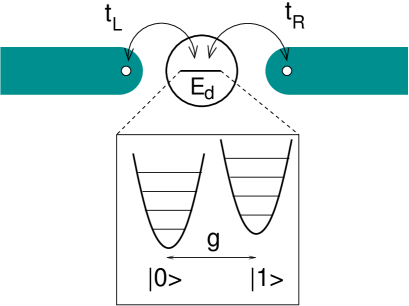
Figure 1: (Color online.) Minimal model of a single-molecular level with energy $E_{d}$ coupled to two leads with tunneling matrix elements $t_{L}$ and $t_{R}$. Depending on the local charge configuration $|0\rangle$ or $|1\rangle$, the Holstein phonon ground state is shifted. The relative displacement between the two configuration is given by the dimensionless electron phonon coupling $g=\lambda_{ph}/\omega_{0}$. The phononic excitations for a fixed charge are multiples of the oscillator energy $\omega_{0}$.

The minimal, non-trivial model for molecular-electronics Galperin et al. (2007); Hützen et al. (2012) comprises a single spinless level whose charge is coupled locally to a single Holstein phonon stemming from the dominating vibrational mode of the molecule. For the current transport this level is coupled to the two leads which are often considered as featureless bands for simplicity. In real materials, band features are important but only influence the single-particle properties which can be accounted for in a frequency dependent charge transfer rate $\Gamma(\omega)$.

This spinless Anderson-Holstein model is depicted schematically in Fig. 1. Depending on the local charge configuration, the local harmonic oscillator is displaced and the distance between the two ground states is given by $g$ (see below.) At the particle-hole symmetric point and in absence of a coupling to the leads, the displaced oscillator ground states are given by the two coherent states $|\pm g/2\rangle$, and we immediately can understand the underlying Franck-Condon physics by the suppression of the overlap $\langle-g/2|g/2\rangle=\exp(-g^{2}/2)$ of the two ground states with increasing electron-phonon coupling $g$.

The spin-less two lead resonant level model (RLM) defined by the Hamiltonian

$$H_{0} = H^{0}_{imp}+H_{T}+H_{leads}$$ (1a)

$$H^{0}_{imp} = E_{d}d^{\dagger}d$$ (1b)

$$H_{T} = \sum_{\alpha=L,R}\frac{t_{\alpha}}{\sqrt{N}}\sum_{k}(d^{\dagger}c_{k\alpha}+c^{\dagger}_{k\alpha}d)$$ (1c)

$$H_{leads} = \sum_{\alpha=L,R}\sum_{k}\varepsilon_{k\alpha}c^{\dagger}_{k\alpha}c_{k\alpha}$$ (1d)

is often usedGalperin et al. (2007); Hützen et al. (2012) as the simplest model to describe quantum transport through a molecule or a suspended nano-bridge.Cuniberti et al. (2005); Leturcq et al. (2009) $d(d^{\dagger})$ annihilates(creates) an electron on the device with energy $E_{d}$, and $c^{\dagger}_{k\alpha}$ creates an electron in the lead $\alpha$ with energy $\varepsilon_{k\alpha}$. The local charge-transfer rate to each lead $\alpha$ is given by $\Gamma_{\alpha}=\pi t_{\alpha}^{2}\rho_{\alpha}(0)$, where $\rho_{\alpha}(\omega)$ is the density of states of lead $\alpha$. Throughout the paper we will use a lead independent constant density of states $\rho_{\alpha}(\omega)=(1/2D)\Theta(D-|\omega|)$ for simplicity; $D$ denotes the band width of both leads.

We only account for a single local vibrational mode with energy $\omega_{0}$ created by $b^{\dagger}$ whose dimensionless displacement operator $\hat{x}=(b^{\dagger}+b)$ is coupled to the density $\hat{n}_{d}=d^{\dagger}d$ of the local level via

$$H_{ph} = \omega_{0}b^{\dagger}b+\lambda_{ph}(b^{\dagger}+b)\left(\hat{n}_{d}-\frac{1}{2}\right)\,\,.$$ (2)

The form of the interaction in (2) ensures particle-hole (PH) symmetry for $E_{d}=0$ and particle-hole symmetric leads.

Focusing only on the local dynamics defined by $H_{imp}=H^{0}_{imp}+H_{ph}$, the harmonic oscillator will be shifted upon changing of the local occupancy away from half filling. This can be made explicit by introducing the arbitrary constant $n_{0}$ and making the trivial substitution

$$d^{\dagger}d-\frac{1}{2} = (d^{\dagger}d-n_{0})+(n_{0}-\frac{1}{2})\;\;.$$ (3)

Then $H_{imp}$ takes the exact form

$$H_{imp} = \omega_{0}\bar{b}^{\dagger}\bar{b}+\lambda_{ph}(\bar{b}^{\dagger}+\bar{b})\left(d^{\dagger}d-n_{0}\right)$$ (4)

$$+\bar{E}_{d}d^{\dagger}d+2E_{p}(n_{0}-\frac{1}{2})^{2}$$

where the displaced phonon is created by $\bar{b}^{\dagger}$ defined as

$$\bar{b}^{\dagger} = b^{\dagger}+g(n_{0}-\frac{1}{2})\,,$$ (5)

and $g=\lambda_{ph}/\omega_{0}$. The new single particle energy $\bar{E}_{d}$

$$\bar{E}_{d} = E_{d}+2\frac{\lambda^{2}_{ph}}{\omega_{0}}(\frac{1}{2}-n_{0})$$ (6)

contains the polaronic energy shift $E_{p}=\frac{\lambda^{2}_{ph}}{\omega_{0}}=\omega_{0}g^{2}$. This polaron shift $E_{p}$ plays an important role of defining the different regimesEidelstein et al. (2013) of the model in addition to the dimensionless coupling constant $g$ and the charge transfer rates $\Gamma_{\alpha}$.

In a mean-field decoupling of the electron-phonon interaction, $n_{0}$ would be replaced by self-consistent local charge expectation $n_{d}=\langle d^{\dagger}d\rangle$ in Eqs. (4-6). A positive (negative) $E_{d}$ leads to a depletion (filling up) of the local level where the effective level $\bar{E}_{d}$ is further shifted to higher (lower) energies by a term proportional to $E_{p}$.

This has a profound impact on the zero-bias conductance as function of the detuning of the level $E_{d}$ by an external gate voltage. The local average occupation $n_{d}$ and therefore, the total displace charge $\Delta N$ due the presence of the impurityLangreth (1966); Anders et al. (1991) is initially controlled by the ratio $E_{d}/\Gamma_{\rm eff}$, where $\Gamma_{\rm eff}$ is the low temperature charge fluctuation scale in the Fermi-liquid fixed point. In the strong coupling regime, $g\gg 1$, the effective level $\bar{E}_{d}$ becomes almost independent of the gate voltage controlling the barelevel $E_{d}$. Hence, the occupation will be nearly independent of $E_{d}$ and, therefore, the conductance will have a plateau unless $|E_{d}|$ exceeds the polaron shift $E_{p}$. The zero-bias conductance depicted in Fig. 13 of Ref. Eidelstein et al., 2013 is a direct consequence of Eq. (6).

We also can use the parametrization of $H_{imp}$ with $n_{0}$ as defined in Eq. (4) to connect $H_{imp}$ with the local molecular Hamiltonian $H_{m}$

$$H_{m} = \omega_{0}b^{\dagger}b+\lambda_{ph}(b^{\dagger}+b)d^{\dagger}d+\varepsilon d^{\dagger}d$$ (7)

often used in the literature. Galperin et al. (2005, 2007); Hützen et al. (2012) Setting $n_{0}=0$, $\varepsilon=E_{d}+E_{p}$ and neglecting the ground state energy shift, $H_{imp}$ becomes identical to $H_{m}$.

Keeping $\varepsilon$ fixed in $H_{m}$ and increasing the electron-phonon coupling $\lambda_{ph}$ as in Ref. Hützen et al., 2012 translates into a renormalization of the single-particle energy by a polaron shift $E_{d}=\varepsilon-E_{p}$ in $H_{imp}$. Starting from $\varepsilon=0$, this implies a population increase of the fermion level upon increase of $\lambda_{ph}$. In this parametrization it becomes apparent that $\lambda_{ph}$ induces a detuning away from particle-hole symmetry.

Combining the RLM as given in Eq. (1) with a coupling to the local Holstein phonon to $H=H_{0}+H_{ph}$ defines the spinless Anderson-Holstein model.

II.2 Lang-Firsov transformation

This Anderson-Holstein model is well studied Hewson and Meyer (2002); Galperin et al. (2007); Hützen et al. (2012); Eidelstein et al. (2013) and a text-book example for an exactly solvable modelMahan (1981) in the limit $t_{\alpha}=0$. Already in the 1960s, it was shown that the local Hamiltonian $H_{imp}=H^{0}_{imp}+H_{ph}$ can be exactly diagonalized using a Lang-Firsov transformation,Lang and Firsov (1962)

$$\hat{U}_{LF} = e^{-g(b^{\dagger}-b)(d^{\dagger}d-\frac{1}{2})}\;\;.$$ (8)

The new elementary excitations are polarons annihilated by the operator $\bar{d}$

$$\bar{d} = \hat{U}_{LF}^{\dagger}\,d\,\hat{U}_{LF}=e^{-g(b^{\dagger}-b)}d$$ (9)

and a free phonon with unrenormalized energy $\omega_{0}$. The polaron shift $E_{p}$ enters the ground state energy. Acting on the bosonic vacuum, the operator $\hat{U}_{LF}=e^{-g(b^{\dagger}-b)(d^{\dagger}d-\frac{1}{2})}$ generates a coherent state $|\pm g/2\rangle$ which describes the ground state of a displaced harmonic oscillator by the dimensionless displacement $\Delta x=\pm g/2$ depending on whether a local charge was present or absent (see also the schematic figure 1.) This reflects the underlying Franck-Condon physics extensively discussed in the literature.Koch and von Oppen (2005); Galperin et al. (2007); Leturcq et al. (2009)

Neglecting the ground state energy shift, the total Hamiltonian $H^{\prime}$ of the impurity coupled to the leads is given by

$$H^{\prime} = H^{\prime}_{imp}+\sum_{\alpha=L,R}\sum_{k}\varepsilon_{k\alpha}c^{\dagger}_{k\alpha}c_{k\alpha}$$

$$+\sum_{\alpha}\frac{t_{\alpha}}{\sqrt{N}}\sum_{k}(e^{g(b^{\dagger}-b)}\bar{d}^{\dagger}c_{k\alpha}+c^{\dagger}_{k\alpha}\bar{d}e^{-g(b^{\dagger}-b)})$$

$$H^{\prime}_{imp} = E_{d}\bar{d}^{\dagger}\bar{d}+\omega_{0}b^{\dagger}b$$ (10)

after the unitary transformation $H^{\prime}=\hat{U}^{\dagger}_{LF}H\hat{U}_{LF}$. We have dropped the bar from the transformed phonon $\bar{b}=\hat{U}^{\dagger}_{LF}b\,\hat{U}_{LF}$ in Eq. (II.2) to keep the notation simple. While the local Hamiltonian $H^{\prime}_{imp}$ became simple and diagonal, we acquired a complicated tunneling term with an exponential electron-phonon coupling $e^{\pm g(b^{\dagger}-b)}$.

Although we have always used the original Hamiltonian in our NRG calculations, the transformed Hamiltonian of Eq. (II.2) is very convenient to gain some deeper insight into the effective low-energy Hamiltonian generated by the renormalization group transformations.This effective model is discussed in detail in Sec. III.1 below.

II.3 Numerical renormalization group and the Anderson Holstein model

The properties of quantum impurity systems such as defined by $H=H_{imp}+H_{T}+H_{leads}$ can be very accurately calculated using the numerical renormalization group. At the heart of this approach is a logarithmic discretization of the continuous bath, controlled by the discretization parameter $\Lambda>1$.Wilson (1975); Bulla et al. (2008) The continuum limit is recovered for $\Lambda\to 1$. Using an appropriate unitary transformation, Wilson (1975) the Hamiltonian is mapped onto a semi-infinite chain, with the impurity coupled to the first chain site. The $N$th link along the chain represents an exponentially decreasing energy scale: $D_{N}\sim\Lambda^{-N/2}$. Using this hierarchy of scales, the sequence of finite-size Hamiltonians ${\cal H}_{N}$ for the $N$-site chain is solved iteratively, discarding the high-energy states at the conclusion of each step to maintain a manageable number of states. The reduced basis set of ${\cal H}_{N}$ so obtained is expected to faithfully describe the spectrum of the full Hamiltonian on a scale of $D_{N}$, corresponding to the temperature $T_{N}\sim D_{N}$. Details can be found on the reviewBulla et al. (2008) by Bulla et al..

Hewson and MeyerHewson and Meyer (2002) pioneered the application of the NRG on the single-lead version of Hamiltonian $H=H_{0}+H_{ph}$. The standard NRG discretisationWilson (1975); Bulla et al. (2008) of $H_{leads}$ maps the model onto a chain Hamiltonian

$$H_{N}\Lambda^{-(N-1)/2} = \tilde{E}_{d}d^{\dagger}d+\tilde{\omega}_{0}b^{\dagger}b+\tilde{\lambda}_{ph}(b^{\dagger}+b)\left(d^{\dagger}d-\frac{1}{2}\right)$$

$$+\sum_{\alpha}V_{\alpha}(d^{\dagger}f_{0\alpha}+f_{0\alpha}^{\dagger}d)$$

$$+\sum_{\alpha}\sum_{n=0}^{N}\Lambda^{-n/2}\bar{\varepsilon}_{n\alpha}f_{n\alpha}^{\dagger}f_{n\alpha}$$

$$+\sum_{\alpha}\sum_{n=0}^{N-1}\Lambda^{-n/2}\bar{t}_{n}(f_{n\alpha}^{\dagger}f_{n+1\alpha}+f_{n+1\alpha}^{\dagger}f_{n\alpha})$$

using a NRG parameter $\Lambda>1$. $\bar{t}_{n},\bar{\varepsilon}_{n}=O(1)$ and $\bar{\varepsilon}_{n}=0$ for PH-symmetric leads. The dimensionless parameters $\tilde{E}_{d},\tilde{\omega}_{0},\tilde{\lambda}_{ph}$ are related to original parametersWilson (1975); Bulla et al. (2008) via the scaling factor $s=D(1+1/\Lambda)/2$: $\tilde{E}_{d}=E_{d}/s,\tilde{\omega}_{0}=\omega_{0}/s,\tilde{\lambda}_{ph}=\lambda_{ph}/s$ and the renormalized tunneling $V_{\alpha}=t_{\alpha}/s$. Using a suitable number of bosonic excitions $N_{b}$, $H_{N}$ is then iteratively diagonalized. A much more detailed introduction to the NRG can be found in the Review by Bulla et al..Wilson (1975); Bulla et al. (2008)

II.4 Scattering-states numerical renormalization group approach to quantum transport

For the calculating of the current $I(V)$ through the molecular level at finite bias $V$ across the two leads, we have used the recently proposed scattering-states numerical renormalization groupAnders (2008a); Schmitt and Anders (2010, 2011) (SNRG) approach to quantum transport. The SNRG is based on an extension of Wilson’s NRG to non-equilibrium dynamics.Anders and Schiller (2005, 2006); Eidelstein et al. (2012) Using the time-evolved density operator, the non-equilibrium steady state retarded Green function can be calculated.Anders (2008b) Below, we only give a rather brief summary of the approach. A more detailed derivation and discussion of the method can be found in Refs. Anders, 2008a; Schmitt and Anders, 2010, 2011.

II.4.1 Definition of the scattering states

In the absence of the electron-phonon interaction the RLM defined in (1) can be diagonalized exactly in the continuum limitHan (2006); Hershfield (1993); Enss et al. (2005); Han and Heary (2007) by the following scattering-states creation operators Oguri (2007); Lebanon et al. (2003); Anders (2008a); Schmitt and Anders (2010)

$$\gamma^{\dagger}_{\varepsilon\alpha} = c^{\dagger}_{\varepsilon\alpha}+t_{\alpha}\sqrt{\rho_{\alpha}(\varepsilon)}G_{0}^{r}(\varepsilon+i\delta)$$

$$\hskip 28.45274pt\times\Bigg{[}d^{\dagger}+\sum_{\alpha^{\prime}}\int d\varepsilon^{\prime}\frac{t_{\alpha^{\prime}}\sqrt{\rho_{\alpha^{\prime}(\varepsilon^{\prime})}}}{\varepsilon+i\delta-\varepsilon^{\prime}}c^{\dagger}_{\varepsilon^{\prime}\alpha^{\prime}}\Bigg{]}\;\;.$$

$\alpha=L(R)$ labels left (right) moving scattering states created by $\gamma^{\dagger}_{\varepsilon\sigma L(R)}$. In this equation, the local retarded resonant-level Green function of the $d$-level

$$G^{r}_{0}(\omega) = \left[\omega+i\delta-E_{d}-\Delta(\omega+i\delta)\right]^{-1}$$ (13)

enters as the expansion coefficient where $\delta>0$ is an infinitesimally small energy scale required to select the correct boundary conditions.

Defining $\bar{t}=\sqrt{t_{L}^{2}+t_{R}^{2}}$, the ratio $r_{R(L)}=t_{R(L)}/\bar{t}$ denotes the relative tunneling strength of each lead $\alpha$ to the impurity $d$-level. The resonant level self energy $\Delta_{\alpha}(\omega+i\delta)$ in $G^{r}_{0}(\omega)$ is given by

$$\Delta(\omega+i\delta) = \bar{t}^{2}\sum_{\alpha}r^{2}_{\alpha}\int d\varepsilon\frac{\rho_{\alpha}(\varepsilon)}{\omega+i\delta-\varepsilon}$$ (14)

$$= \Re e[\Delta(\omega)]-i\Gamma(\omega)$$

and its imaginary part $\Gamma(\omega)$ denotes the energy dependent charge-fluctuation scale which becomes a constant in the wide-band limes of a featureless band.

In the limit of infinitely large leads the single-particle spectrum remains unaltered, and these scattering states diagonalize the Hamiltonian (1)

$${\cal H}_{0}={\cal H}(\lambda_{ph}=0) = \sum_{\alpha=L,R}\int d\varepsilon\,\varepsilon\gamma^{\dagger}_{\varepsilon\alpha}\gamma_{\varepsilon\alpha}$$ (15)

up to a neglected ground state energy shift.Schweber (1962)

The creation operator $\gamma^{\dagger}_{\varepsilon\alpha}$ is a solution of the operator Lippmann-Schwinger equationSchweber (1962) and, therefore, the corresponding state break time-reversal symmetry. The necessary boundary condition for describing a current-carrying open quantum system is encoded in the small imaginary part $+i\delta$ entering Eq. (II.4.1-14) required for convergence when performing the continuum limit ${\rm Vol.}\to\infty$. Since left and right movers at the same energy are time-reversal pairs, time-reversal symmetry is restored at zero bias yielding a exactly vanishing net current in that limit.

To avoid possible bound states, we will only consider the wide-band limit: $D\gg{\rm max}\{|\varepsilon_{d}|,\Gamma_{\alpha},|V|\}$. Furthermore, $\Gamma_{0}=\Gamma(0)=\Gamma_{L}+\Gamma_{R}$ is used as energy unit in this paper. We measure the coupling asymmetry by the ratio $R=\Gamma_{L}/\Gamma_{R}$. A perfect unitary limit of $e^{2}/h$ conductance quantum can only be reached for $R=1$ with $R\to\infty$ and $R\to 0$ correspond to the tunneling regime.

Hershfield has shown that the steady-state density operator for a current-carrying non-interacting quantum system retains its Boltzmannian formHershfield (1993)

$$\hat{\rho}_{0} = \frac{e^{-\beta({\cal H}_{0}-\hat{Y}_{0})}}{\textrm{Tr}\left[e^{-\beta({\cal H}_{0}-\hat{Y}_{0})}\right]}\,,\,$$

$$\hat{Y}_{0} = \sum_{\alpha\sigma}\mu_{\alpha}\int d\varepsilon\,\gamma^{\dagger}_{\varepsilon\sigma\alpha}\gamma_{\varepsilon\sigma\alpha}$$ (16)

at finite bias. The $\hat{Y}_{0}$ operator accounts for the different occupation of the left-moving and right-moving scattering states. $\mu_{\alpha}$ denote the different chemical potentials of the leads. Since $H_{0}$ is bilinear, the transport is perfectly ballistic and the total current is given by the difference between the current to the left and the current to the right.

All steady-state expectation values of any operator are calculated using $\hat{\rho}_{0}$ for the non-interacting problem which includes the finite bias. In the absence of the electron-phonon interaction this is a trivial and well-understood problem. It was shownOguri (2007) that the current obtained with this density-operator $\hat{\rho}_{0}$ is identical to the current calculated using a generalized Landauer formula based on Keldysh Green functions.Hershfield et al. (1991); Meir and Wingreen (1992); Wingreen and Meir (1994)

This form of $\hat{\rho}_{0}$ stated in Eq. (16) remains valid even for the fully interacting systemHershfield (1993) when replacing ${\cal H}_{0}\to{\cal H}$, and replacing $Y_{0}\to Y$. Since the $Y$ must be constructed from the many-body scattering states, its explicit analytical expression is unknown for a general Hamiltonian $H$ of an interacting systems.

We, therefore, proceed in two steps using the arguments outlined in the literature.Hershfield (1993); Doyon and Andrei (2006) At first, we add to $H_{0}$ a fictitious electron-phonon interaction term $H_{e-ph}^{\prime}$ which commutes with $Y_{0}$, i.e.  $[H_{e-ph}^{\prime},Y_{0}]=0$. Hershfield’s argument also yields a steady-state density operator of the form $\hat{\rho}^{\prime}_{0}=\exp[-\beta({\cal H}_{0}+H^{\prime}_{e-ph}-\hat{Y}_{0})]/Z$. For the model under consideration we have chosen

$$H^{\prime}_{e-ph}=\omega_{0}b^{\dagger}b+\lambda_{ph}(b^{\dagger}+b)\left(\sum_{\alpha=L,R}r_{\alpha}^{2}d^{\dagger}_{\alpha}d_{\alpha}-\frac{1}{2}\right)$$ (17)

where the $d_{\alpha}$ are the operators obtained from inverting Eq. (II.4.1)

$$d_{\alpha} = \bar{t}\int d\varepsilon\sqrt{\rho(\varepsilon)}[G^{r}_{0}(\varepsilon)]^{*}\gamma_{\varepsilon\alpha}\,$$ (18)

which fulfill the anti-commutation relation $\{d_{\alpha},d^{\dagger}_{\beta}\}=\delta_{\alpha\beta}$. The annihilation operator $d$ of a local electron on the device is reconstructed by the linear combination of its left-mover and right-mover contributions $d=r_{R}d_{R}+r_{L}d_{L}$. We note that $H^{\prime}_{e-ph}$ approaches $H_{e-ph}$ in the extreme tunneling limit of $R\to\infty$ (or $R\to 0$.)

In a second step, we perform the time evolution of $\hat{\rho}^{\prime}_{0}$ with respect to the fully interacting Hamiltonian to infinitely long time: the density operator $\hat{\rho}(t)$ progresses from its initial value $\hat{\rho}^{\prime}_{0}$ at $t=0$ as

$$\hat{\rho}(t) = e^{-i{\cal H}_{f}t}\hat{\rho}^{\prime}_{0}e^{i{\cal H}_{f}t}$$ (19)

where we set $\hbar=1$.

II.4.2 Scattering-states numerical renormalization group

The basic idea of the scattering-states numerical renormalization group (SNRG) approach is summarized as follows.

(I) Knowing the analytical form of the non-equilibrium density operator $\hat{\rho}^{\prime}_{0}$, we can discretize scattering states on a logarithmic energy mesh identically as in the standard NRGBulla et al. (2008); Anders (2008a) and perform a standard NRG using $K_{0}={\cal H}(\lambda_{ph}=0)+H^{\prime}_{e-ph}-\hat{Y}_{0}$. The density operator $\hat{\rho}^{\prime}_{0}(V)$ contains all information about the current carrying steady-state for the Hamiltonian $K_{0}+Y_{0}$.Hershfield (1993)

(II) Starting at time $t=0$, we let the system evolve with respect to the full Hamiltonian ${{\cal H}_{f}}=H(\lambda_{ph}>0)$ Then, the density operator $\hat{\rho}(t)$ progresses from its initial value $\hat{\rho}^{\prime}_{0}$ at $t=0$ according to Eq. (19). Since we quench the system only locally, it is a fair assumption that $\hat{\rho}(t)$ reaches a steady-state at $t\to\infty$ independent of initial condition for an infinitely large system, since all bath correlation functions must decay for infinitely long times.

The finite size oscillations always present in the NRG calculation Anders (2008a) are projected out by defining the time-averaged density operator

$$\hat{\rho}_{\infty} = \lim_{\tau\to\infty}\frac{1}{\tau}\int_{0}^{\tau}dt\hat{\rho}(t)\,.$$ (20)

As a consequence, only the matrix elements diagonal in energy contribute for $t\to\infty$ in accordance with the steady-state condition

$$[{\cal H}_{f},\hat{\rho}_{\infty}] = 0\,\,.$$ (21)

Even though $\hat{\rho}_{\infty}$ remains unknown analytically, we can explicitly construct it numerically using the time-dependent NRGAnders and Schiller (2005, 2006); Eidelstein et al. (2012) (TD-NRG.)

(III) The steady-state retarded Green function is defined as

$$G^{r}_{A,B}(t) = -i\textrm{Tr}\left[\hat{\rho}_{\infty}[\hat{A}(t),\hat{B}]_{s}\right]\Theta(t),$$ (22)

where $\hat{A}(t)=e^{i{\cal H}_{f}t}\hat{A}e^{-i{\cal H}_{f}t}$, $[\hat{A}(t),\hat{B}]_{s}$ denotes the commutator ($s=-1$) for bosonic, and the anti-commutator ($s=1$) for fermionic correlation functions. This Green function can be calculated using the time-dependent NRGAnders and Schiller (2005, 2006) and extending ideas developed for equilibrium Green functions.Peters et al. (2006) The details of the algorithm is derived in Ref. Anders, 2008b.

II.4.3 Current as function of the bias voltage

The current $I_{\alpha}$ is defined as a charge currentMeir and Wingreen (1992) from the lead $\alpha$ to the local $d$-level. It has been shownMeir and Wingreen (1992); Hershfield (1993); Oguri (2007) that for the model investigated here, the symmetrized current

$$I = r^{2}_{R}I_{L}-r^{2}_{L}I_{R}\quad.$$ (23)

is related to the steady-state spectral function of the local level, $\rho_{d}(\omega,V)=\Im m[G^{r}_{\sigma}(\omega-i0^{+},V)]/\pi$ by a generalized Landauer formula

$$I(V) = \frac{G_{0}}{e}\int_{-\infty}^{\infty}\,d\omega\,\left[f_{R}(\omega)-f_{L}(\omega)\right]\Gamma_{0}\pi\rho_{d}(\omega,V)$$ (24)

where $f_{\alpha}(\omega)=f(\omega-\mu_{\alpha})$. The prefactor

$$G_{0} = \frac{e^{2}}{h}\frac{4\Gamma_{L}\Gamma_{R}}{\Gamma_{0}^{2}}$$ (25)

measures the asymmetry of the junction. $G_{0}$ reaches the universal conductance quantum $e^{2}/h$ for a symmetric point-contact junction, i. e. $\Gamma_{L}=\Gamma_{R}$, and is strongly suppressed in the tunneling regime $\Gamma_{\alpha}\ll\Gamma_{-\alpha}$. The two chemical potentials $\mu_{\alpha}$ are set to $\mu_{L}=-r^{2}_{R}V$ and $\mu_{R}=r^{2}_{L}V$ as function of the external source-drain voltage $V$ consistent with a serial-resistor model which is required by the current conservation $I_{R}=-I_{L}$.

While the conserving Keldysh Green function approach treats the problem of initially decoupled leads and propagate the system to a current-carrying steady state, the scattering states NRG starts from an initial current carrying steady state of the non-interacting problem. Employing the TD-NRGAnders and Schiller (2005, 2006) we let the system evolve by calculating the full density operator $\hat{\rho}(t)$ numerically in the limit of $t\to\infty$ using the Hamiltonian of the interacting system.

In a continuum limit, any correlation function will have a finite correlation time above which the memory of this initial state will be lost. Hershfield (1993); Doyon and Andrei (2006) As a consequence, a unique steady state is approached which is compatible with the imposed boundary condition as pointed out by Hersfield. Hershfield (1993); Doyon and Andrei (2006) Our starting point is therefore identical to any approach using a propagation along a Keldysh contour.Keldysh (1965) The differences arise from the inevitable approximations made in Keldysh perturbation theory by selecting a subclass of diagrams for a practical calculation of the non-equilibrium self-energies. In contrast, our approach does not make any of such approximations and, therefore, includes the full interaction to infinitely high order. It only comprise a systematic but well controlled error stemming from discretization of the bath continuumBulla et al. (2008); Eidelstein et al. (2012); Guettge et al. (2012) inherent any NRG (or DMRGSchollwöck (2005)) approach.

A hysteretic behaviorLi et al. (2003) is observed in some molecular junctions when sweeping the voltage a very slow but finite rate. Using a simple mean-field approximation, the possibility of polaron formation on a molecular wire has been proposed as a mechanism for the observe NDR.Galperin et al. (2005) Such hysteretic behavior in self-consistent equation can also occur in the employed approximations when increasing the coupling constant beyond the validity range of such approximations. Such many-valued solution might not survive in an exact solution of the problem and their robustness need to be checked against the inclusion of higher order contributions. A prominent example of such a known false hysteresis in the I-V characteristics is the GW-approach to Anderson model out of equilibrium.Spataru et al. (2009)

The theoretical description of such hysteretic behavior requires tracing the same experimental conditions in the simulations. Starting from the initial condition of a fully interacting current-carrying steady state for a given bias voltage the time dependent current $I(V(t),t)$ must be calculated for a given rate of voltage change.

In a recent paper by Muehlbacher et al.Albrecht et al. (2012) it has been proposed that signatures of bistability in non-equilibrium charge transport through molecular quantum dots might be linked to subtle differences in the initial conditions. This, however, is clearly beyond our scattering-states approach which targets exclusively the stationary steady-state limit.

III Equilibrium renormalization group approach

Before we present the results for the quantum transport in Sec. V, we briefly review the equilibrium parameter flow of the model. This provides the necessary understanding of the energy scales and defines the different regime which become relevant for the quantum transport.

III.1 Low energy Hamiltonian

While Hewson and Meyer investigated the equilibrium dynamics of the more complex spin-full modelHewson and Meyer (2002) using the NRG, we focus on the simpler spin-less model in this work. Its low energy fixed point is also given by an effective resonant level model. In the limit $\omega_{0}>D,\Gamma_{0}$, its effective tunneling matrix elements $t^{\rm eff}_{\alpha}$ are estimated by using $H^{\prime}$ defined in Eqn. (II.2): the local phonons are approximately in their ground state, and

$$t_{\alpha}\to t^{\rm eff}_{\alpha} \approx t_{\alpha}\langle 0|\exp(-g(b^{\dagger}-b))|0\rangle$$ (26)

$$= t_{\alpha}\exp(-\frac{g^{2}}{2})\;\;.$$

In leading order, we obtain the renormalized charge fluctuation scale $\Gamma_{\rm eff}\approx\Gamma_{0}\exp(-g^{2})$ in this limit.

By expanding the factor

$$e^{-g(b^{\dagger}-b)} = 1-g(b^{\dagger}-b)+O\left(g^{2}\right)$$ (27)

for small $g\ll 1$ added by the Lang-Firsov transformation to the tunneling term

$$H^{\prime}_{T} = \sum_{\alpha}t_{\alpha}(e^{g(b^{\dagger}-b)}\bar{d}^{\dagger}c_{0\alpha}+c^{\dagger}_{0\alpha}\bar{d}e^{-g(b^{\dagger}-b)})\,\,,$$ (28)

it is apparent that an effective repulsive Coulomb interaction term

$$H_{U} = \sum_{\alpha}U_{\rm eff}(d^{\dagger}d-\frac{1}{2})(n_{0\alpha}-\frac{1}{2})$$ (29)

is obtained in second-order perturbation theory in $g$. Of course, this type of effective interaction and all possible higher order contribution will be automatically generated by RG transformation in each NRG iteration step. Taking into account the renormalization of the tunneling matrix element $t_{\alpha}\to t^{\rm eff}_{\alpha}$, we conjecture that $U_{\rm eff}$ generated in the RG transformation is given by

$$U_{\rm eff} \propto \left(\sum_{\alpha}t_{\alpha}^{\rm eff}g\right)^{2}\frac{1}{\omega_{0}}$$ (30)

in leading order. Then, the dimensionless Coulomb repulsion reads

$$\frac{U_{\rm eff}}{D} = \frac{\pi}{2}\frac{\Gamma_{\rm eff}}{\omega_{0}}g^{2}f(x)=\frac{U_{ana}}{D}f(x)$$ (31)

where $f(x)$ is an unknown scaling function of order $O(1)$ which accounts for higher order corrections in the expansion (27). The analysis of the NRG data, presented below suggests that the scaling variable is given by $x=\alpha(\omega_{0}/\Gamma_{0})g^{2}$ in the anti-adiabatic regime $\omega_{0}\gg\Gamma_{0}$. The function $\alpha(y)$ is a slow varying function of the order $O(1)$ as shown in Sec. III.3.

A perturbative treatmentEidelstein et al. (2013) to second order in $t_{\alpha}$, predicts $U_{\rm eff}/D\approx(4\Gamma_{0}E_{p})/(\pi\omega_{0}^{2})$ in the weak coupling limit, i. e. $g\ll 1$, and $U_{\rm eff}/D\approx(4\Gamma_{0}/E_{p})$ in the strong coupling limit, $g\gg 1$. Note that these results are only valid as long as $\Gamma_{0}$ is the smallest energy scale and, therefore, $U_{\rm eff}/D$ remains a perturbative correction in the validity range of the perturbation theory. This analytic result agrees nicely with our conjecture of Eq. (31) which will be backed up by our extensive NRG study below.

Note, however, that the values for $U_{\rm eff}/D$ extracted from the full NRG calculation can result in magnitudes of $O(1)$ and, therefore, this regime would be beyond the reach of a second-order perturbation theory. Nevertheless, the leading-order scaling with the model parameters remains well captured by Eq. (31) as long as $\omega_{0}/\Gamma_{0}>1$.

III.2 Renormalized parameters

In equilibrium, the anti-binding combination of lead operators, $c_{0-}=r_{L}c_{0R}-r_{R}c_{0L}$ decouples from the impurity, and we are left with an effective one-band model since the local $d$-orbital is only connected to orthogonal combination $c_{0+}=r_{R}c_{0R}+r_{L}c_{0L}$. Therefore, we focus on an effective one-band model but with the charge-transfer rate $\Gamma_{0}+\Gamma_{L}+\Gamma_{R}$.

Eidelstein et al.Eidelstein et al. (2013) have already pointed out that the low-energy Hamiltonian of the spinless one lead Anderson Holstein model can be mapped onto an effective interacting resonant level model (IRLM)

$$H^{\rm IRLM} = H_{0}+H_{imp}$$

$$H_{0} = \sum_{k}\varepsilon_{k}c^{\dagger}_{k}c_{k}$$ (32)

$$+t_{\rm eff}(d^{\dagger}c_{0}+c^{\dagger}_{0}d)$$

$$H_{imp} = \tilde{\epsilon}_{d}d^{\dagger}d+U_{\rm eff}(d^{\dagger}d-\frac{1}{2})(c^{\dagger}_{0}c_{0}-\frac{1}{2})$$

for effective band width $D_{\rm eff}<\omega_{0}$. Its parameters $\tilde{\varepsilon}_{d},t_{\rm eff}$ and $U_{\rm eff}$ can be extracted in different ways from the NRG level spectrum.Wilson (1975); Hewson and Meyer (2002); Bulla et al. (2008); Eidelstein et al. (2013)

In Ref. Eidelstein et al., 2013, the effective parameter $\Gamma_{\rm eff}\propto t^{2}_{\rm eff}$ is extracted from the charge susceptibilty at the particle-hole symmetric point. We, however, use a different approach which allows for a definition of $\Gamma_{\rm eff}$ for arbitrary values of $E_{d}$, away from the particle-hole symmetric point by applying the procedure proposed by Hewson et al..Hewson et al. (2004)

In this method the renormalized parameters are extracted directly from the NRG level flow. It is based on the analytically known low-energy stable Fermi-liquid fixed pointBulla et al. (2008) and the exact solution of the RLM for a given NRG chain. The discretized effective RLM for the fixed-point dynamics,

$$H_{N}^{RLM}\Lambda^{-(N-1)/2} = \tilde{\varepsilon}_{d}d^{\dagger}d+t_{\rm eff}(d^{\dagger}f_{0}+f_{0}^{\dagger}d)$$

$$+\sum_{n=0}^{N}\Lambda^{-n/2}\bar{\varepsilon}_{n}f_{n}^{\dagger}f_{n}$$

$$+\sum_{n=0}^{N-1}\Lambda^{-n/2}\bar{t}_{n}(f_{n}^{\dagger}f_{n+1}+f_{n+1}^{\dagger}f_{n})\,,$$

is exactly diagonalizedWilson (1975); Bulla et al. (2008) to

$$H_{N}^{RLM} = \sum_{l=1}^{\frac{N+2}{2}}\left(\varepsilon_{p,l}e^{\dagger}_{l}e_{l}+\varepsilon_{h,l}h^{\dagger}_{l}h_{l}\right)$$ (34)

for a NRG chain with odd number of lead sites – $N$ even. $e^{\dagger}_{l}$ ($h^{\dagger}_{l}$) creates the $l$-th elementary particle (hole) excitation with the energy $\varepsilon_{p,l}$ ($\varepsilon_{h,l}$.) Obviously, the impurity Green function $G^{N}_{d}(z)$

$$G^{N}_{d}(z) = \frac{1}{z-\tilde{\varepsilon}_{d}\Lambda^{(N-1)/2}-[V_{\rm eff}]^{2}\Lambda^{N-1}g_{0}(z)}$$ (35)

must have poles at these single-particle excitation energies $z=\varepsilon_{e,l},\varepsilon_{h,l}$. $g_{0}(z)$ is the Green function at chain site $n=0$ in the absence of the impurity and can be calculated by a continuous fraction expansion.Hewson et al. (2004)

The first single-particle excitation, $E_{1p}$, and the first single-hole excitation of the NRG level spectrum, $E_{1h}$ respectively, are very good approximation of $\varepsilon_{p,1}$ and $\varepsilon_{h,l}$ close to the Fermi-liquid fixed point. These two NRG energies are sufficient to determine the two unknown effective parameters $\tilde{\varepsilon}_{d}$ and $V_{\rm eff}$ by solving the two coupled algebraic equationsHewson et al. (2004)

$$\frac{E_{1p}\Lambda^{-(N-1)/2}}{2\Gamma_{\rm eff}(N)}-\frac{\tilde{\varepsilon}_{d}(N)}{2\Gamma_{\rm eff}(N)} = \frac{\Lambda^{(N-1)/2}}{\pi}g_{0}(E_{1p})$$ (36)

$$\frac{-E_{1h}\Lambda^{-(N-1)/2}}{2\Gamma_{\rm eff}(N)}-\frac{\tilde{\varepsilon}_{d}(N)}{2\Gamma_{\rm eff}(N)} = \frac{\Lambda^{(N-1)/2}}{\pi}g_{0}(-E_{1h})$$

for the poles of the Green function, where $\Gamma_{\rm eff}=\pi t_{\rm eff}^{2}\rho(0)$. Note, that these are dimensionless parameters, all given in units of $D(1+1/\Lambda)/2$.

In order to calculate $U_{\rm eff}$, we analyze the four eigenstates of $H_{0}^{{\rm IRLM}}$ comprising only the local level and $f_{0}$. It is easy to see that $U_{\rm eff}$ is related to the energy difference between the lowest particle-hole excitation and the sum of a single-particle and a single-hole excitation. The adaptation of equation (18) in Ref. [Hewson et al., 2004]

$$E_{1p}+E_{1h}-E_{1ph}=2U_{\rm eff}(N)\Lambda^{(N-1)/2}$$

$$\times\left(|\psi_{d,p}(1)|^{2}|\psi_{c,h}(1)|^{2}+|\psi_{d,h}(1)|^{2}|\psi_{c,p}(1)|^{2}\right)\,\,$$ (37)

requires the knowledge of expansion coefficients $\psi_{d,p}(l)$ of the annihilation operator $d$

$$d = \sum_{l=1}^{(N+2)/2}\left(\psi_{d,p}(l)e_{p,l}+\psi_{d,h}(l)h^{\dagger}_{h,l}\right)$$ (38)

and $\psi_{c,p}(l)$ of the first lead chain site $n=0$

$$f_{0} = \sum_{l=1}^{(N+2)/2}\left(\psi_{0,p}(l)e_{p,l}+\psi_{0,h}(l)h^{\dagger}_{h,l}\right)$$ (39)

in terms of the elementary excitation of the low-energy fixed point Hamiltonian (34). The coefficients $|\psi_{d,p}(l)|^{2}$ are determined by the weights of the poles of the finite size chain impurity Green functions

$$G^{N}_{d}(z) = \sum_{l=1}^{(N+2)/2}\left(\frac{|\psi_{d,p}(l)|^{2}}{z-e_{p,l}}+\frac{|\psi_{d,h}(l)|^{2}}{z-e_{h,l}}\right)$$ (40)

and coefficients $|\psi_{c,h}(l)|^{2}$ by the corresponding Green functions of the first lead site $n=0$, $G^{N}_{c}(z)$, which is related to the local $T$-matrix $V^{2}G_{d}^{N}(z)$

$$G^{N}_{c}(z) = g_{0}(z)+V_{\rm eff}\Lambda^{N-1}G^{N}_{d}(z)g^{2}_{0}(z)$$

$$= g_{0}(z)\left[\frac{z-\tilde{\varepsilon}_{d}^{\rm eff}\Lambda^{(N-1)/2}}{z-\tilde{\varepsilon}_{d}^{\rm eff}\Lambda^{(N-1)/2}-[V_{\rm eff}]^{2}\Lambda^{N-1}g_{0}(z)}\right]$$

Using the calculated parameters $\tilde{\varepsilon}_{d}(N)$ and $\Gamma^{\rm eff}(N)$, the spectral weights at the pole $\varepsilon_{p,1}$ are approximately given by

$$|\psi_{d,p}(1)|^{2} = \frac{1}{1-[V_{\rm eff}]^{2}\Lambda^{N-1}g^{\prime}_{0}(E_{1p})}$$

$$|\psi_{c,p}(1)|^{2} = g_{0}(E_{1p})\frac{E_{1p}-\tilde{\varepsilon}_{d}\Lambda^{(N-1)/2}}{1-[V_{\rm eff}]^{2}\Lambda^{N-1}g^{\prime}_{0}(E_{1p})}$$ (42)

and analog for $\varepsilon_{h,1}$. We have replaced the true single-particle (single-hole) excitation energy $\varepsilon_{p,1}$ ($\varepsilon_{h,l}$) by the first NRG particle (hole) excitation energy $E_{1p}$ ($E_{1h}$.) Thereby, $g^{\prime}_{0}(z)$ denotes the derivative of $g_{0}(z)$.

III.3 NRG analysis of the renormalized parameter

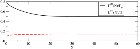
Figure 2: (Color online.) Example NRG flow for $U(N)/D$ and $\Gamma_{\rm eff}(N)$ vs NRG iteration $N$ for the parameters $\omega_{0}/\Gamma_{0}=\lambda_{ph}/\Gamma_{0}=5$.

In this section, we present the results for the renormalized parameter for the low-energy equilibrium Hamiltonian extracted from the NRG level spectrum of the single-lead model as described in section III.2. We have used $\Lambda=1.5$, kept $N_{s}=1500$ NRG states after each iteration, and included the lowest $N_{b}=400$ local phonon states. The band-width of a lead with constant DOS $\rho(\omega)=\Theta(D-|\omega|)/2D$ was set to $D=100\Gamma_{0}$, and $\Gamma_{0}$ serves as energy scale throughout the paper. In this section, we only investigate the PH-symmetric limit by setting $E_{d}=0$.

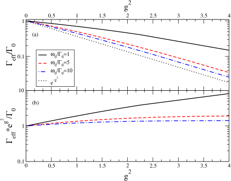
Figure 3: (Color online.) (a) Anti-adiabatic and crossover regime: $\Gamma_{\rm eff}$ as function of $g^{2}=(\lambda_{ph}/\omega_{0})^{2}$ for $\omega_{0}/\Gamma_{0}=1,5,10$, (b) rescaled $\Gamma_{\rm eff}e^{g^{2}}$ vs $g^{2}$; (c) $\Gamma_{\rm eff}/\Gamma_{0}$ vs $E_{\rm p}$ in the adiabatic regime. The correction factor $\alpha(\omega_{0}=0.2)=1.02,\alpha(\omega_{0}=0.3)=0.93$. In the anti-adiabatic and the crossover regime, (a) and (b) $N_{s}=1500$, in the adiabatic regime (c) we kept $N_{s}=2500$ NRG states for accuracy.

In Fig. 2, the flow of $\Gamma_{\rm eff}(N)$ and $U_{\rm eff}(N)$ is depicted with respect to the NRG iteration $N$ for one specific parameter set, $\omega_{0}/\Gamma_{0}=\lambda_{ph}/\Gamma_{0}=5$. Fast convergence is achieved when approaching the low-energy fixed point for $N\to\infty$. We have extracted the fixed point values of $\varepsilon^{\rm eff}_{d}=\lim_{N\to\infty}\tilde{\varepsilon}_{d}^{\rm eff}(N)$, $\Gamma_{\rm eff}=\lim_{N\to\infty}\Gamma_{\rm eff}(N)$, $U_{\rm eff}=\lim_{N\to\infty}U_{\rm eff}(N)$ for various values of the electron-phonon coupling $\lambda_{ph}$ and $\omega_{0}$. Since, $\varepsilon^{\rm eff}_{d}=0$ for all PH-symmetric parameters, we do not show any results. In the ph-asymmetric regime, $\varepsilon^{\rm eff}_{d}\neq 0$ measures the effective PH-symmetry breaking external field.

The results for $\Gamma_{\rm eff}/\Gamma_{0}$ vs $g^{2}$ are shown in Fig. 3(a) for three different phonon frequencies $\omega_{0}/\Gamma_{0}=1,5,10$. For $\Gamma_{0}\ll\omega_{0}$, we approach the anti-adiabatic limit in which the phonons can almost instantaneously react on the charge fluctuations. The data suggests that $\Gamma_{\rm eff}\approx\Gamma_{0}\exp[-g^{2}]$ for $\omega_{0}\to\infty$ and weak and moderate values of $g$. The closer $\omega_{0}$ approaches the charge-fluctuation scale $\Gamma_{0}$, the stronger the deviations for this approximation. In the context of the spin-full model, Hewson et al. Hewson and Meyer (2002) have already proposed a modification of the exponent $\exp(-g^{2})\to\exp(-g^{2}h(\lambda_{ph},\omega_{0}))$ by a function $h$ which accounts for the additional correction. For large $\omega_{0}$, the leading contribution to $h$ is a constant approaching $1$, however, we were not able to find a universal scaling function $h$ using our data which describes the crossover from weak to strong coupling, $g<1$ and $g>1$ respectively .

Restricting to the strong coupling limit, however, Eidelstein et al. Eidelstein et al. (2013) were able to show that all graphs $\Gamma_{\rm eff}(g,\omega_{0})$ collapse onto a single curve by introducing the universal function through the expression $\Gamma_{\rm eff}/\Gamma=\exp[-g^{2}F(R)]$. The dimensionless parameter $R=\Gamma_{0}/E_{p}$ emphasizes the importance of the polaronic energy shift $E_{p}$ for the physics of the model.

The validity range of such a universal function $F(R)$ requires $R\ll 1$. For $R\to 1$, however, significant deviations from a universal scaling are already observed in Ref. Eidelstein et al., 2013.

Since we focus on the regime $R>1$, the study by Eidelstein et al. Eidelstein et al. (2013) investigates the complementary strong-coupling regime to our weak and intermediate coupling regime. Although the equilibrium NRG can reach $R\ll 1$ as recently demonstrated, the TD-NRG and the SNRG are restricted to moderate values of $g$ due to the increasing of discretization artefacts.Eidelstein et al. (2012); Guettge et al. (2012)

In the adiabatic regime, $\omega_{0}\ll\Gamma_{0}$, field-theoretical argumentsVinkler et al. (2012) have been employed to show

$$\Gamma_{\rm eff} \approx \Gamma_{0}\left(1-\frac{2}{\pi}\frac{E_{\rm p}}{\Gamma_{0}}\right)$$ (43)

for ${max}\{E_{\rm p}/\Gamma_{0},g,E_{d}/\Gamma_{0}\}\ll 1$. Our numerical analysis for the adiabatic regime agrees with that perturbative result, but we find a prefactor of $1/2$ up to very small corrections instead of $2/\pi$ stated in Eq. (43), as shown in Fig. 3(c). In the analytical calculationVinkler et al. (2012) the local Lorentzian spectral function was approximated by a simple constant $\rho$ while in our numerics the full energy dependency enters the calculations which probably accounts for the difference. Our data provides evidence for a crossover from a perturbative $[1-\alpha\frac{E_{p}}{\Gamma_{0}}]$ correction factor to $\Gamma_{0}$ with $\alpha\approx 1/2$ in the adiabatic regime to an exponential suppression factor $\exp[-g^{2}h(\lambda_{ph},\omega_{0})]$ in the anti-adiabatic regime.

Let us now discuss $U_{\rm eff}$ dynamically generated by the electron-phonon interaction. The plot in Fig. 2 demonstrates clearly that such an effective Coulomb repulsion $U(N)$ can be extracted directly from the NRG level flow via Eq. (III.2) and converges rather quickly to a low temperature fixed point value $U_{\rm eff}$.

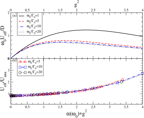
Figure 4: (Color online.) (a) $\omega_{0}U_{\rm eff}$ as function of $g^{2}$ for four different values of $\omega_{0}/\Gamma_{0}=1,5,10,20$. (b) $f(x)=U_{\rm eff}/U_{ana}$ as defined in Eq. (31) vs $\alpha(\omega_{0})g^{2}$, where we used the scaling factor $\alpha(\omega_{0})=0.85,1,1.1$ for $\omega_{0}/\Gamma_{0}=5,10,20$. NRG parameters as in Fig. 3.

The results for $\omega_{0}\,U_{\rm eff}$ are depicted in Fig. 4(a) for four different values of $\omega_{0}$. Qualitatively, the results can be understood by the conjectured form

$$\frac{U_{\rm ana}}{D} = \frac{\pi}{2}\frac{\Gamma_{\rm eff}}{\omega_{0}}g^{2}=\frac{\pi}{2}\frac{\Gamma_{\rm eff}E_{p}}{\omega^{2}_{0}}\,.$$

of Eq. (31) above where $U_{\rm eff}\propto U_{\rm ana}$. $\omega_{0}U_{\rm eff}$ increases linearly with $x=g^{2}$ and is exponentially suppressed for large $x$ due to the renormalization of the bare hopping constant. Focusing only on the three graphs in the anti-adiabatic regime $\omega_{0}>\Gamma_{0}$, we plot the ratio $U_{\rm eff}/U_{\rm ana}$ as function of $\alpha(\omega_{0})x$.

By an appropriate dimensionless scale $\alpha(\omega_{0})$ which only depends on the phonon frequency, we are able to rescale $x$ such that all ratios $U_{\rm eff}/U_{ana}$ collapse onto one universal scaling curve of the order $O(1)$ in this regime as shown in Fig.  4(b).

The simple arguments leading to the estimated analytical value $U_{ana}$ do not hold in the extended anti-adiabatic and in the crossover regime, and this mapping onto the universal scaling curve fails for $\omega_{0}/\Gamma_{0}=1$. As indicated already in Fig. 4(a), $U_{\rm eff}$ is much larger and the additional renormalization for $\Gamma_{\rm eff}$ by the finite $U_{\rm eff}$ in the effective IRLM might have to be taken into account when crossing over to the adiabatic regime $\omega_{0}<\Gamma_{0}$.

IV Equilibrium spectral functions

IV.1 Technical details

Since the equilibrium spectral functions are used to calculate the zero-bias conductance within the linear response theory, we present some local spectra to set the stage for the non-equilibrium transport. Furthermore, we also can use the direct calculation of the equilibrium spectral function as a benchmark for testing the quality of the non-equilibrium spectra obtained by the time-dependent NRG approachAnders and Schiller (2005, 2006) to non-equilibrium Green functions.Anders (2008b)

For two trivial limits, exact solutions are analytically known. (i) In the absence of the coupling to the leads, $t_{\alpha}=0$, the exact solution of the local spectral functionMahan (1981) comprises of a set of equidistant $\delta$-peaks separated by the phonon-frequency $\omega_{0}$. Their spectral weights are given by modified Bessel functions whose arguments are temperature dependent.Mahan (1981) (ii) In the opposite limit, $\lambda_{ph}=0$, the spectral function of is simply given by the Lorentzian of the RLM which will be weakly modified for $0<g\ll 1$.

We have used the complete Fock space algorithmPeters et al. (2006); Anders (2008b); Weichselbaum and von Delft (2007) to calculate the NRG spectral function. The $\delta$-functions of the spectral function have been replaced by the standard NRG broadening function

$$\delta(\omega\pm|\omega_{n}|) \to \frac{\exp(-b^{2}/4)}{b|\omega_{n}|\sqrt{\pi}}e^{-[\frac{1}{b}\log(|\omega/\omega_{n}|]^{2}}$$ (44)

characterized by the broadening parameter $b$ and additionally averaged over $N_{z}$ different band discretizations.Yoshida et al. (1990); Anders and Schiller (2005, 2006) The equation of motionBulla et al. (1998) exactly relates the self-energy

$$\Sigma^{\rm ph}(z) = \lambda_{ph}\frac{F(z)}{G_{d}(z)}$$ (45)

to ratio of the correlation function

$$F(z)=\ll\!\!(b+b^{\dagger})d|d^{\dagger}\!\!\gg(z)$$ (46)

and the local Green function $G_{d}(z)=\ll\!\!d|d^{\dagger}\!\!\gg(z)$.

For $\lambda_{ph}=0$, the correlation function $F(z)$ vanishes: it is generated in first order by the electron phonon coupling. Therefore, $F(z)\propto\lambda_{ph}$ in leading order which immediately reproduces the leading order of magnitude of $\Sigma^{\rm ph}(z)\propto\lambda_{ph}^{2}$ for the weak coupling regime $\lambda_{ph}/\Gamma_{0}\ll 1$ obtained from perturbation theoryCaroli et al. (1971) where the leading order Feynman diagram is depicted in Fig. 6.

The spectral functions discussed below are all obtained from $G_{d}(z)=[z-E_{d}-\Delta(z)-\Sigma^{\rm ph}(z)]^{-1}$ where the total self-energy is given by the sum of $\Sigma^{\rm ph}(z)$ and $\Delta(z)$ defined in Eq. (14). In our numerics we evaluate the Green function very close to the real axis and $\rho_{d}(\omega)=\Im mG_{d}(\omega-i\delta)/\pi$ using a very small value for $\delta/\Gamma_{0}=10^{-10}-10^{-7}$.

IV.2 Particle-hole symmetry

IV.2.1 Crossover regime

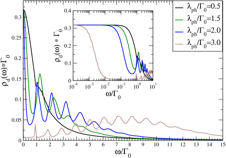
Figure 5: (Color online.) Equilibrium spectral functions for $E_{d}=0$, $\omega_{0}/\Gamma_{0}=1$ and various values of $\lambda_{ph}/\Gamma_{0}=0.5,1.5,2,3$. NRG parameter: $N_{s}=1200$, $\Lambda=1.5$, $N_{b}=80$, $N_{z}=512$, $b=0.03$.

In Fig. 5, the positive part of the symmetric local spectral function $\rho_{d}(\omega)=\Im mG_{d}(\omega-i\delta)/\pi$ is depicted for a series of electron-phonon couplings $\lambda_{ph}/\Gamma_{0}=0.5,1.5,2.0,3.0$ and a fixed phonon frequency $\omega_{0}/\Gamma_{0}=1$. For $\lambda_{ph}/\Gamma_{0}=0.5$, the RLM Lorentzian is broadened and a kink at $\omega\approx\omega_{0}$ is related to a sharp rise of the self-energy at $\omega$. With increasing $\lambda_{ph}$, more and more phonon replica of the resonance peak $\omega=E_{d}=0$ are visible and their width increasingly narrows which is related to the narrowing of the central peak as depicted in the inset. Obviously the central peak width is given by the low temperature fixed point value $\Gamma_{\rm eff}$ which is already exponentially suppressed for $\lambda_{ph}/\Gamma_{0}=3$.

We have used a very large number of $N_{z}=512$ values in combination with a very small broadening $b=0.03$ for the $z$-averaging of the spectral functions to ensure that the spectra depicted in Fig. 5 are really nearly broadening independent even at higher frequencies.

The spectral peak at $\omega=0$ remains pinned at its universal value for $T=0$ in accordance with the Friedel sum-rule.Langreth (1966); Anders et al. (1991); Eidelstein et al. (2013) The spectral weight of this zero-frequency peak, however, is reduced to $\Gamma_{\rm eff}/\Gamma_{0}$ and redistributed to the higher energy phonon replica peaks.

For $\lambda_{ph}/\Gamma_{0}=3$, we checked in several very long NRG runs averaging up to $N_{z}=1024$ bath discretizations and using a very small broadening parameter of $b=0.01$ that the line width of the high energy phonon peaks are independent of the NRG broadening selected in Fig. 5.

The increase of the spectral function and the maxima of the envelop functions at $\omega\approx\pm 8\Gamma_{0}$ is related to the finite $U_{\rm eff}$. Considering only the two local orbitals, $d$ and $c_{0}$, of the IRLM (III.2) which defines the initial NRG Hamiltonian $H_{0}^{NRG}$ of the IRLM model, one can calculate the spectral functions exactly and finds single-particle excitations at $\omega_{N}\approx\pm U(N)/2$. Since the value of $U(N)$ can strongly depend on the iteration and approaches its fixed point value $U_{\rm eff}$ only for $|\omega|\ll\Gamma^{\rm eff}$, the peak positions correspond to the value of the renormalized $U(N)/2$ where the NRG iteration $N$ corresponds to the energy scale $\omega\approx\omega_{N}\propto\Lambda^{-(N-1)/2}$. This is in complete analogy to the single-impurity Anderson model where the bare high-energy value of $U$ defines the location of the high-energy charge excitation peaks, while the low-energy fixed point value of $U_{\rm siam}^{\rm eff}\approx T_{K}$ as shown by Hewson et al.Hewson et al. (2004)

Although Fig. 4(a) indicates that for $\lambda_{ph}/\Gamma_{0}=3$, $U_{\rm eff}$ is significantly lower than for the smaller values $\lambda_{ph}/\Gamma_{0}=1.5,2$, no additional charge peaks are found for the latter parameters. This is related to the fact that the self-energy contribution $\Sigma^{\rm ph}(z)$ is proportional to $\lambda_{ph}^{2}$ in leading order. If the magnitude of the self-energy is too small, the renormalized resonant level width $\Gamma(N)$ dominates the envelop function. Once $g>1$, $\Gamma_{0}$ evidently becomes significantly suppressed, and spectral weight is increasingly shifted to higher frequencies. The broad phonon side peaks become observable once $\Gamma_{\rm eff}\ll\Gamma_{0}$ and the central resonance lost much of its weight.

IV.2.2 Weak coupling regime

Figure 6: Feynman diagram of the electron-phonon self-energy $\Sigma^{\rm ph}(z)$ in $\lambda_{ph}^{2}$, including the two attached incoming and outgoing electron-propagator lines. The full line represents the local Green function $G_{d}(z)$, the wiggled line the phonon-propagator.

In the weak coupling regime, $g^{2}\ll 1$, the spectral function is only slightly altered by the electron-phonon coupling. Starting from the free Green function of the RLM, the second-order contribution to the self-energy is given by the Feynman diagram shownin Fig. 6. Evaluating this leading order text-book diagramMahan (1981) yields the analytical expression

$$\Im m\Sigma^{\rm ph}(\omega-i\delta) = \pi\lambda_{ph}^{2}[g(\omega_{0})+f(\omega+\omega_{0})]\rho_{d}(\omega+\omega_{0})$$

$$+\pi\lambda_{ph}^{2}[g(\omega_{0})+f(\omega_{0}-\omega)]\rho_{d}(\omega-\omega_{0})$$

where $f(\omega)$ ($g(\omega)$) is the Fermi (Bose) function. The self-energy essentially vanished for $|\omega|<\omega_{0}$ and $T\to 0$ and acquires a significant value only for $|\omega|>\omega_{0}$. The sharpness of the increase is governed by the Fermi function: an energy quantum of at least one bosonic excitation energy $\omega_{0}$ is needed to open up the additional decay channel.

In a conserving approximation, one would replace the phonon propagator by its fully dressed version which includes the shift of the phonon frequencies as well as a finite life-time broadening due to the local particle-hole excitations. This effect of the charge susceptibility has been neglected in Eq. (IV.2.2). If we include this effect we would need to convolute $\Im m\Sigma^{\rm ph}(\omega-i\delta)$ with the true phonon spectral function which has been replaced by $\delta$-functions in the derivation of Eq. (IV.2.2). Therefore, we expect (i) a broadening of the steep increase above $\omega_{0}$ with increasing $\lambda_{ph}$ as well as additional features at multiples of the phonon frequency, since $\Sigma^{\rm ph}(\omega-i\delta)$ will also enter self-consistently the charge susceptibility.

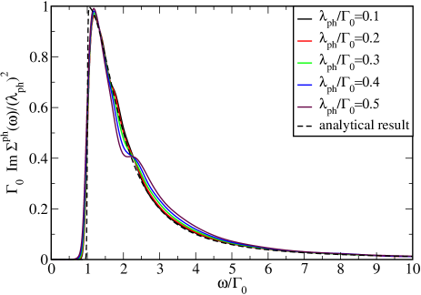
Figure 7: (Color online.) Imaginary part of self-energy contribution $\Sigma^{\rm ph}(\omega-i\delta)$ for $E_{d}=0$, $\omega_{0}=\Gamma_{0}$ and various values of $\lambda_{ph}$ in the weak coupling regime $\lambda_{ph}/\Gamma_{0}<1$ and positive frequencies. The dashed line depicts the analytic self-energy given by Eq. (IV.2.2) and evaluated for the same temperature $T=8.5\times 10^{-3}\Gamma_{0}$ as the NRG results. NRG parameter: $N_{s}=1500$, $\Lambda=1.6$, $N_{b}=40$, $N_{z}=8$, $b=0.1$.

In Fig. 7, the self-energy contribution $\Im m\Sigma^{\rm ph}(\omega-i\delta)$ close to the real axis is depicted for few values $(\lambda_{ph}/\Gamma_{0})^{2}\ll 1$. Dividing out the leading order prefactor, $\lambda_{ph}^{2}$, the magnitude of self-energy becomes nearly independent of $\lambda_{ph}$. The analytical expression of Eq. (IV.2.2) added as dashed line shows a remarkably good agreement with the NRG self-energy obtained via Eq. (45). Due to the broadening, the NRG self-energy cannot generate the same steep increase of the self-energy at $\omega\approx\omega_{0}$. Note, that a shoulder is slowly developing at $\omega\approx 2\omega_{0}$ with increasing $\lambda_{ph}$, a precursor of additional phonon-peaks in the spectra. This is due to higher order processes not included in the second-order perturbation expansion, but present in a proper conserving approximation for $\Sigma^{\rm ph}(z)$.

IV.3 Particle-hole asymmetry

Recently, Hützen et al. Hützen et al. (2012) investigated the I-V characteristics of the spin-less Anderson-Holstein model using an iterative real-time path integral approach.Weiss et al. (2008) Within this approach the current is directly calculated using a generating functional, and no spectral functions are required. Signatures of a Franck-Condon blockade have been reported using the local molecular Hamiltonian $H_{m}$

$$H_{m} = \omega_{0}b^{\dagger}b+\lambda_{ph}(b^{\dagger}+b)d^{\dagger}d+\varepsilon d^{\dagger}d$$

defined in Eq. (7) for the parameters $\varepsilon=0$ and $\omega_{0}=2\Gamma_{0}$: the suppression of the currentHützen et al. (2012) has been found when increasing the electron-phonon coupling $\lambda_{ph}$. Since $H_{imp}$ is identical to $H_{m}$ by setting $n_{0}=0$ and $E_{d}=\varepsilon-E_{p}$, the suppression of the current at zero bias can be partially understood in terms of the polaronic shift of the single-particle energy $E_{d}=\varepsilon-g^{2}\omega_{0}$. Increasing $\lambda_{ph}$ decreases $E_{d}$ for constant $\varepsilon$ and, therefore, increases the particle-hole asymmetry. As a consequence, the stronger the electron-phonon coupling, the more energy is required to depopulate the level.

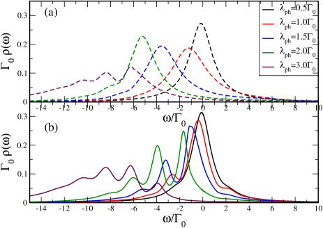
Figure 8: (Color online.) Equilibrium spectral function for the molecular impurity Hamiltonian $H_{m}$, Eq. (7) from weak to strong coupling in the anti-adiabatic regime $\omega_{0}=2\Gamma_{0}$. The solid lines in (b) show spectra at $T=0.2\Gamma_{0}$, the dashed lines in (a) the spectra for $T=1.2\Gamma_{0}$. With $\varepsilon=0$ and $n_{0}=0$, $E_{d}$ is given by $E_{d}=-g^{2}w_{0}$ in $H_{imp}$. NRG parameter: as in Fig. 7.

The spectral functions are shown for two different temperatures and $\varepsilon=0$ and $\omega_{0}=2\Gamma_{0}$ in Fig. 8. With increasing $\lambda_{ph}$, the main resonance peak is shifted to lower energies by $E_{p}$. Additional phonon-side peaks occur asymmetrically around the main resonance at $E_{d}$. The decrease of the spectra at $\omega=0$ is clearly visible translating immediately to the reportedHützen et al. (2012) suppression of the zero bias conductance. By comparing Fig. 8(a) and (b), we also note an increasing shift of the spectra toward the chemical potential and a visible narrowing of the main resonance when lowering the temperature for fixed $\lambda_{ph}$.

IV.4 Benchmark for non-equilibrium spectral functions

The scattering states NRG approach to quantum transportAnders (2008a); Schmitt and Anders (2010, 2011) relies on the analytically known density operator of a non-interacting model at finite bias.Hershfield (1993) It is evolved to the density-matrix of the fully interacting problem using the TD-NRG.Anders and Schiller (2005, 2006) This non-equilibrium density operator for the limit $t\to\infty$ is used to calculate the finite-bias retarded spectral function entering the equation (24) for the current-voltage characteristic of the junction.Meir and Wingreen (1992)

The restriction to the single-lead version of the Hamiltonian defined in Eq. (1) in the absence of a bias can be used to benchmark the quality of the non-equilibrium spectra function algorithm and its limits. Starting from a decoupled electron-phonon system, $\lambda_{ph}=0$, and letting the system evolve using the full Anderson-Holstein model $H=H_{0}+H_{ph}$, we must recover the equilibrium dynamics of $H$ for $t\to\infty$. Therefore, we compare the results for the spectral function obtained from the standard equilibrium NRG algorithmPeters et al. (2006) with the spectra obtained from a extension of the TD-NRG to spectral functions.Anders (2008b)

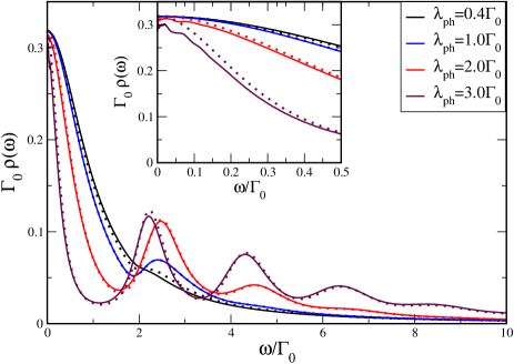
Figure 9: (Color online.) Comparison between the equilibrium and non-equilibrium spectral function for a single lead and the phonon energy $\omega_{0}=2\Gamma_{0}$. The dotted lines show the equilibrium spectral function, the solid lines with the same color the spectra obtained for times $t\to\infty$ after a quench by switching on the electron-phonon coupling at time $t=0$. NRG parameter: $N_{s}=1500$, $\Lambda=1.6$, $N_{b}=40$, $N_{z}=8$, $b=0.1$, $T=8.5\times 10^{-3}\Gamma_{0}$.

The results for $\omega_{0}=2\Gamma_{0}$, $E_{d}=0$ and various electron-phonon coupling constants $\lambda_{ph}$ are depicted in Fig. 9. The dotted line shows the equilibrium spectral function, the solid line the spectra obtained from a quench by switching on the electron-phonon coupling at $t=0$. The agreement remains very good even at high energies up to moderate values of $\lambda_{ph}$.

The larger the phonon frequency, the better the agreement between the direct calculation of equilibrium spectra and the spectra obtained by the non-equilibrium approach. For small $\omega_{0}\leq\Gamma_{0}$, however, the non-equilibrium approach has its limitations. The number of bosonic Fock states which are required even in equilibrium grows significantly. For our equilibrium calculation, we needed already $N_{b}=400$ states, in a recent study,Eidelstein et al. (2013) the rather very generous choice of NRG parameter, $N_{b}=3000$ and $N_{s}=8000$, have been used in a single lead model but no z-averaging was required for the thermodynamical properties investigated in that paper. For the required z-averaging over 64 discretizations in an TD-NRG calculation, this would be computationally much to expensive and is, therefore, beyond the reach of our approach.

V Quantum transport: Results

V.1 Scattering-states NRG

This section is devoted to the results of the non-linear I-V characteristics calculated using the SNRG. The differential conductance $G(V)=dI/dV$ has been obtained numerically from the I(V) curves.

Section V.1.1, is devoted to the particle-hole symmetric regime of the model, i. e. $E_{d}=0$. We investigate the evolution of the I-V characteristics from a junction with symmetric couplings ($R=1$) to the tunneling regime ($R\to\infty$.) In Sec. V.1.2 we focus on the PH-asymmetric model and investigate the Franck-Condon blockade for $\varepsilon=E_{d}-E_{p}=0$ and a finite electron-phonon coupling.

V.1.1 Particle-hole symmetric model

The electrical current calculated via Eq. (24) is shown as a function of the applied bias in Fig. 10(a) for three different ratios of $R=\Gamma_{L}/\Gamma_{R}$, a phonon frequency $\omega_{0}=2\Gamma_{0}$ and a fixed electron-phonon coupling $g=1$. For better comparison, the prefactor $G_{0}$ defined in Eq.  (25), has been divided out. $G_{0}$ only contains the trivial reduction of the current upon increasing of $R$ starting from its maximum of $e^{2}/h$ for $R=1$. For a PH-symmetric Hamiltonian, the current remains PH-symmetric even for an asymmetric junction as can be seen analytically from Eq. (24).

The differential conductance $G(V)=dI/dV$ depicted in Fig. 10(b) has been obtained by numerically differentiating the data of Fig. 10(a). For a better comparison, we added the corresponding equilibrium transmission function obtained from the spectral function shown in the Fig. 9.

Particle-hole symmetry and a Fermi-liquid equilibrium ground state yields a pinned peak at zero bias which approaches $G_{0}$ for $T\to 0$ which can be understand quite easily by applying the Friedel sum rule.Langreth (1966); Anders et al. (1991) The narrowing of the central resonance due to the renormalization of $\Gamma_{0}\to\Gamma_{\rm eff}$, exemplified in Fig. 9 prevails also in the differential conductance.

Qualitatively, $G(V)$ traces the transmission function $T(\omega)=\pi\Gamma_{0}\rho(\omega)$ but quantitatively significant differences are observed. The additional transmission maxima are clearly visible at finite voltage which are related to phonon-assisted tunneling increasing significantly the current above a threshold. This threshold position depend on the asymmetry $R$ of the junction.

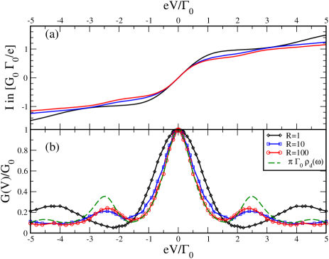
Figure 10: (Color online.) (a) I(V) for the symmetric model, i. e. $E_{d}=0$, and three different ratios $R=\Gamma_{L}/\Gamma_{R}=1,10,100$. The vibrational parameters are $\omega_{0}=\lambda_{ph}=2\Gamma_{0}$. (b) $dI/dV$ in units of $G_{0}$ as function of $eV$ obtained by numerically differentiating the curves in (a). Additionally, the equilibrium transmission function $T(\omega)=\pi\Gamma_{0}\rho_{d}(\omega)$ obtained from the spectral function $\rho_{d}(\omega)$ of Fig. 9 has been added for comparison. NRG parameter: $N_{s}=2000$, $\Lambda=2$, $N_{b}=35$, $N_{z}=64$, $b=0.15$, $T=6.5\times 10^{-3}\Gamma_{0}$.

We expect that $G_{0}^{-1}dI/dV$ approaches the equilibrium transmission function in the tunneling regime $R\to\infty$ and $T\to 0$. This is clearly the case for $R=100$ and low voltages. We note, however, that the peak position of first maxima at $eV\approx\pm\omega_{0}$ is well reproduced but the peak height is smaller than expected from the equilibrium transmission function $T(\omega)=\pi\Gamma_{0}\rho_{d}(\omega)$. This might be caused by remaining non-equilibrium effects still relevant for $R=100$. However, we believe that this is cause by the limitations of the numerical accuracy of the SNRG at large bias caused by the discretisation and the broadening of the spectral function in combination with the TD-NRG time evolution.

By decreasing the asymmetry from $R=100$ to $R=10$ small differences are visible which can be traced back mainly to the changes chemical potentials $\mu_{L}$ and $\mu_{R}$ for the same voltage drop. For a symmetric junction $R=1$, the strongest non-equilibrium effects are observed. $G(V)$ does not follow the expectation $G(V)\propto[T(eV/2)+T(-eV/2)]$ where the equilibrium transmission function $T(\omega)$ naively has replaced full bias dependent spectra $\rho_{d}(\omega,V)$ in Eq. (24). The width of the central peak is smaller that expected for $G(V)\propto[T(eV/2)]$ and the peaks from the phonon assisted tunneling occur closer to $\pm 2\omega_{0}$ as suggested by the equilibrium transmission function. This is due to a significant change of the non-equilibrium spectral function with increasing bias voltage. Spectral weight is redistributed to higher frequency due to backscattering processes for which additional phase space becomes available at finite voltage.

The full width at half maximum (FWHM) of the zero bias $dI/dV$ peak is not simply given by $2\Gamma_{\rm eff}$ as suggested by a simple generalization of equilibrium spectral function. Non-equilibrium effects cause a bias dependency of the spectral function: the width of $dI/dV$ is significantly smaller than predicted from such a naive $[T(eV/2)+T(-eV/2)]$ fit to $G(V)$ for $R=1$.

V.1.2 Particle-hole asymmetric model

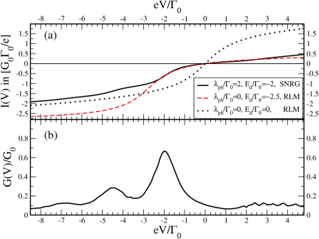
Figure 11: (Color online.) (a) I(V) for the particle-hole asymmetric model, $E_{d}/\Gamma_{0}=-2(\varepsilon=0)$ and an asymmetric junction $R=\Gamma_{L}/\Gamma_{R}=10$. The vibrational parameter are $\omega_{0}=2\Gamma_{0}$, and $\lambda_{ph}=2\Gamma_{0}$. The solid line shows the SNRG current, The black dotted line indicates the $\lambda_{ph}=\varepsilon=0$ current, the blue dashed line current for a shifted level $E_{s}/\Gamma_{0}=-2.5$ in an non-interacting junction (RLM)at $T=0$. (b) $dI/dV$ in units of $G_{0}$ as function of $eV$ obtained by numerically differentiating the SNRG curve in (a). NRG parameter: as in Fig. 10.

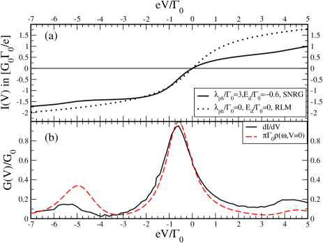
Figure 12: (Color online.) (a) I(V) for $E_{d}/\Gamma_{0}=-0.6(\varepsilon/\Gamma_{0}=1.65)$ and $R=\Gamma_{L}/\Gamma_{R}=10$. The vibrational parameter are $\omega_{0}=4\Gamma_{0}$, and $\lambda_{ph}=3\Gamma_{0}$. The solid line shows the SNRG current, The black dotted line indicates the $\lambda_{ph}=\varepsilon=0$ current (RLM) at $T=0$. (b) $dI/dV$ in units of $G_{0}$ as function of $eV$ obtained by numerically differentiating the SNRG curve in (a). NRG parameter: as in Fig. 10.

For a particle-hole asymmetric regime of the model and asymmetric lead couplings, the current as function of the applied bias voltage and corresponding the differential conductance $G(V)$ is depicted in Fig. 11. We have set $\varepsilon=0$ in $H_{m}$ in resonance with both chemical potentials at zero bias, the phonon frequency to $\omega_{0}/\Gamma_{0}=2$ and selected a moderate electron-phonon coupling $g=\lambda_{ph}/\omega_{0}=1$. As discussed before, the bare single-particle level $\varepsilon$ is shifted by the polaron energy to $E_{d}=-E_{p}=-2\Gamma_{0}$. The corresponding equilibrium spectral function has been plotted in Fig. 8 which clearly documents the significant asymmetry.

The strong suppression of the current with increasing $\lambda_{ph}$ and fixed $\varepsilon$, as seen by comparing the $\lambda_{ph}=0$ and $\lambda_{ph}/\Gamma_{0}=2$ curves has been interpreted as Franck-Condon blockade physics.Hützen et al. (2012) Clearly, the leading order effect stems from a polaronic shift $E_{p}$ of the single-particle level. The SNRG curve tracks the current through a shifted level at $E_{d}/\Gamma_{0}=-2.5$ and $\lambda_{ph}=0$ rather well for positive voltages as indicated by the read dashed line.

We have already seen in the equilibrium spectral function – green curve in Fig. 8 – that the electron-phonon interaction causes a redistribution of spectral weight below the chemical potential. Each phonon peak contains only of a fraction of the spectral weight, and spectral weight has been shifted even below $-10\Gamma_{0}$ which contribute only at much larger negative voltages. In the asymmetric junction ($R=10$), the current $|I|$ increases significantly for $eV<-E_{p}$. However, the magnitude of current clearly remains lower than the reference current (dashed line) for a non-interacting shifted level. This is consistent with the the qualitativ features of the equilibrium spectra and leads to the Franck-Condon current suppression of the current at small and intermediate bias voltage. A second phonon induced maximum in $G(V)$ is found below $V<-E_{p}-\omega_{0}$ and corresponds to the second peak in the spectral function. A very shallow maximum at $eV/\Gamma_{0}\approx-7$ could be related to the third phonon peak in the spectral function. We believe, that the small oscillations in die $dI/dV$ curve for positive bias voltage has no physical significance and is caused by the numerical differentiation of the numerical I-V data.

Maintaining the same coupling asymmetry $R=10$ but increasing the phonon energy to $\omega_{0}/\Gamma_{0}=4$, the current vs voltage is depicted in Fig. 12(a) and the corresponding $dI/dV$ curve in Fig. 12(b) for a moderate electron phonon coupling $g=0.75$. We also added the equilibrium spectral function to the (b) as a comparison. Since $R=10$, $d\rho(\omega,V)/dV$ remains significant, and $dI/dV$ does not trace the equilibrium spectra $\rho(\omega,V=0)$. There remains a significant renormalization of the spectral function for a moderate asymmetry which only must vanish in the limit $R\to\infty$ or $R\to 0$.

V.2 Tunneling limit for the crossover regime

In the adiabatic regime the physics is dominated by the charge-fluctuation scale $\Gamma_{0}$ being the largest local energy scale in the problem. The weak electron-phonon coupling causes only small renormalization of the electronic and phononic degrees of freedom. In this regime, Keldysh approaches have been successfully applied to the problem: the phonon frequency is reduced by particle-hole excitations in leading order which is well captured already in conserving one-loop diagramsCaroli et al. (1971, 1972); Galperin et al. (2007) for the electron and the phonon propagator.

Recently, it was shownEidelstein et al. (2013) that the anti-adiabatic regime extends from $\omega_{0}>\Gamma_{0}$ to $\omega_{0}\approx O(\Gamma)$, as long as the polaronic shift $E_{p}$ exceeds the charge-fluctuation scale. The crossover regime from this extended anti-adiabatic regime to the adiabatic regime where the polaron contains less and less phononic excitations has been definedEidelstein et al. (2013) by the parameter hierarchy $E_{p}>\Gamma_{0}>\omega_{0}$ and $\Gamma_{\rm eff}\approx\omega_{0}$.

Although this regime is accessible to the equilibrium NRG, a very large number of phononic states are needed for accurately tracking the equilibrium flow.Eidelstein et al. (2013) The SNRG relies on the switching on the electron-phonon coupling and let the system evolve from a $\lambda_{ph}=0$ to a finite $\lambda_{ph}$. Apparently, the TD-NRG is not able to reproduce reliably the equilibrium Green functions for larger electron-phonon couplings in the crossover regime. This might also be related to the logarithmic discretisation of the scattering states in combination with the change of the ground statesEidelstein et al. (2012); Guettge et al. (2012)

Therefore, we have focused on the tunneling regime ($R\to\infty$) where the retarded Green function becomes bias independent and $\rho_{d}(\omega,V)$ can be replaced in Eq. (24) by $\rho_{d}(\omega,V=0)$. We have included $N_{b}=300$ phonon Fock states and kept $N_{s}=2500$ NRG after each iteration to calculate the equilibrium spectra using only a single-lead.

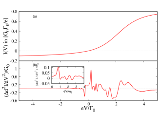
Figure 13: (a) I(V) for the particle-hole asymmetric model, $E_{d}/\Gamma_{0}=1.2$ in the crossover regime. The phonon energy $\omega_{0}=0.26\Gamma_{0}$, and $\lambda_{\mathrm{ph}}=0.6\Gamma_{0}$. (b) $\Delta\mathrm{d}^{2}I/\mathrm{d}V^{2}$ in units of $G_{0}$ as a function of eV obtained by taking analytically the second derivative of Eq. (24) in the limit $R\to\infty$. NRG parameter: $N_{\mathrm{s}}=2500,\Lambda=1.8,N_{\mathrm{b}}=300,N_{\mathrm{z}}=8,b=0.1,T=8\times 10^{-4}\Gamma_{0}$.

Since the charge-fluctuation scale $\Gamma_{0}$ is the dominating energy scale, $G(V)$ is unsuitable to reveal subtle inelastic processes induced by the electron-phonon coupling in the cross-over regime. The information about the inelastic processes, however, is encoded in the second derivativeCaroli et al. (1971, 1972); Galperin et al. (2007) of the $I(V)$ curve, $\mathrm{d}^{2}I/\mathrm{d}V^{2}$.

For the tunneling $I(V)$ is depicted in Fig. 13(a). Although, $\omega_{0}<\Gamma_{0}$, the polaron shift is given by $E_{p}/\Gamma_{0}=1.38$ and exceeds $\Gamma_{0}$, while the renormalized $\Gamma_{\rm eff}$ remains above $\omega_{0}$. Therefore, the choice of parameters lies in the crossover regime between the extended anti-adiabatic and the adiabatic regime.

Since $\mathrm{d}^{2}I/\mathrm{d}V^{2}$ is up to some smaller voltage dependence proportional to the derivative of the spectral function, it is sensitive to the derivative to the phonon self-energy. Although, this absolute magnitude is small, its derivative can be huge if it contains a threshold set by a Fermi-function shifted by one or multiples of the phonon frequencies. In second order Keldysh approximation, these steep features dominate $\mathrm{d}^{2}I/\mathrm{d}V^{2}$ on voltages $eV/\omega_{0}\approx O(1)$ as seen in Fig. 11 of Ref. Galperin et al., 2007. The sign change of the $\mathrm{d}^{2}I/\mathrm{d}V^{2}$ for small voltages can only occur for very pronounce changes in the self-energies.

In the NRG, the features are much less dominant: the method has its limitation due to the discretization and the artificial broadening which puts limit to the gradient of any self-energy change as already discussed above. In order to extract some information about inelastic scattering processes, we have calculated $\mathrm{d}^{2}I_{0}/\mathrm{d}V^{2}$ by using a Lorentz fit to the spectral function centered around $\bar{E}_{d}$ which is the mean-field (MF) reference value. Now we calculate the full $\mathrm{d}^{2}I/\mathrm{d}V^{2}$ and define $\Delta\mathrm{d}^{2}I/\mathrm{d}V^{2}=\mathrm{d}^{2}I/\mathrm{d}V^{2}-\mathrm{d}^{2}I_{0}/\mathrm{d}V^{2}$ as difference between the full second derivative and the MF result. This is plotted in Fig. 13(b). Now we notice the sharp features around $eV=\pm\omega_{0}$ and at multiples of the phonon frequencies. This is clearly visible in the inset of Fig. 13(b) where the bias is measured in units of $\omega_{0}$. While for $\lambda_{ph}\to 0$, the self-energy is dominated by threshold of the inelastic processes at $|\omega|=\omega_{0}$, for increasing $\lambda_{ph}$ multiple phonon absorption and emission processes start to contribute to the self-energy. Similar to Fig. 7 where two phonon processes are clearly visible, this multi-phonon processes at moderate coupling yield the additional features in $\Delta\mathrm{d}^{2}I/\mathrm{d}V^{2}$. The one and two-phonon processes have been also seen in a much more pronounce manner in the literatureGalperin et al. (2007) using Keldysh perturbation theory.

VI Discussion and outlook

We have extended the scattering states NRG to the charge-transport through a molecular junction. To set the stage for the non-linear transport results, we have provided a detailed analysis of the low-temperature equilibrium physics of the spin-less Anderson-Holstein model from an NRG perspective. We have shown that the model can been mapped onto an interacting resonant level model in the extended anti-adiabatic regime and extracted the renormalized charge-transfer scale $\Gamma_{\rm eff}$ and the effective Coulomb interaction $U_{\rm eff}$ in a regime complementary to the recent study of Eidelstein et al..Eidelstein et al. (2013)

We have calculated the equilibrium spectral functions and used those to benchmark our non-equilibrium algorithm.Anders (2008b) We have demonstrated that for the weak coupling limit, $(\lambda_{ph}/\omega_{0})^{2}\ll 1$, the NRG tracks perfectly the self-energy obtained from the second-order Feynman diagram. For large electron-phonon couplings the typical phonon replica peaks of the exact atomic solutionLang and Firsov (1962); Mahan (1981) are found. Using extensive z-averging the spectra become independent of the NRG broadening even at higher frequencies.

Exemplified in Fig. 10, the reduction of the charge-transfer scale $\Gamma_{\rm eff}$ due to the electron-phonon coupling in the equilibrium properties conveys into a narrowing of the differential conductance. In contrary to a recent QMC studyHan (2010) for the spin-full model with Coulomb interaction, our results clearly show the phonon side peaks expected from the equilibrium spectra. The location, however, depends on the two chemical potentials as well as the coupling asymmetry of the junction.

Gating the junction away from the particle-hole symmetric point reveals the Franck-Condon blockade physics with increasing electron-phonon coupling. The leading order effect is understood in terms of a polaronic level shift, and the I(V) curve tracks a shifted resonant level model for positive bias voltages. For negative bias, however, the current is suppressed due to a redistribution of spectral weight to higher frequencies.