Experimental study of parametric subharmonic instability for internal plane waves

Abstract

Internal waves are believed to be of primary importance as they affect ocean mixing and energy transport. Several processes can lead to the breaking of internal waves and they usually involve non linear interactions between waves. In this work, we study experimentally the parametric subharmonic instability (PSI), which provides an efficient mechanism to transfer energy from large to smaller scales. It corresponds to the destabilization of a primary plane wave and the spontaneous emission of two secondary waves, of lower frequencies and different wave vectors. Using a time-frequency analysis, we observe the time evolution of the secondary waves, thus measuring the growth rate of the instability. In addition, a Hilbert transform method allows the measurement of the different wave vectors. We compare these measurements with theoretical predictions, and study the dependence of the instability with primary wave frequency and amplitude, revealing a possible effect of the confinement due to the finite size of the beam, on the selection of the unstable mode.

1 Introduction

An essential ingredient of the thermohaline circulation is the mechanism by which the denser water that was produced in the high latitude regions (colder and saltier), once it has flowed down the continental slopes towards the abyssal ocean, can come back to the surface to close the loop. This process involves an energy input to provide the gain of potential energy necessary to lift this denser water. It is believed that turbulent mixing, generated by wind and tides, is the mechanism that performs this task (Munk, 1966; Munk & Wunsch, 1998). One possible way is via the breaking of internal gravity waves (Staquet & Sommeria, 2002), ubiquitous in the ocean, allowing a transfer of energy from large scales to small scales, where this energy is partly dissipated in heat and partly converted in potential energy through diapycnal mixing.

The detailed mechanisms for energy dissipation of internal gravity waves is still debated. Several mechanisms have been proposed:

• parametric subharmonic instability (MacKinnon & Winters, 2005; Alford et al., 2007),

• reflection on sloping boundaries (Dauxois & Young, 1999),

• scattering by mesoscale structures (Rainville & Pinkel, 2006b),

• small scale bathymetry (Kunze & Smith, 2004; Johnston et al., 2003; Peacock et al., 2009).

The importance of these four possible dissipative processes has to be estimated and compared precisely. It is likely that a combination of them might be the correct answer but the usual physicists’ approach, aiming at separating the different processes one by one, is presumably appropriate in a first stage.

Parametric subharmonic instability (PSI) is the resonant mechanism by which a primary wave is unstable to infinitesimal perturbations, transferring energy through the quadratic nonlinearity of the Navier-Stokes equation to two secondary waves, satisfying temporal and spatial resonant conditions. More precisely, PSI is the class of resonant wave-wave interactions wherein energy is transferred from large scale to smaller scales and where the frequencies of the secondary waves are near half the primary frequency. Studying the particular case of a primary plane wave is very interesting since a plane wave is solution of the full inviscid nonlinear equation for any amplitude. However, as will be discussed below, this solution becomes unstable above a given threshold, which can be computed analytically (McEwan et al., 1972).

Initially, this instability was considered only for the gravity or capillary waves (McGoldrick (1965)). However, Hasselmann (1967) proved that this instability could be observed in many physical systems, and in particular for internal waves. Following this initial report, several theoretical studies have been developed for this phenomenon, deriving in particular the expression for the growth rate in presence (or absence) of viscosity (Thorpe, 1968; McEwan, 1971; McEwan et al., 1972; McEwan & Plumb, 1977). At the same time, the first experimental observations of the instability have been reported (McEwan, 1971; McEwan et al., 1972; McEwan & Plumb, 1977; Benielli & Sommeria, 1998). These first observations allowed the determination of the amplitude threshold of the instability and the temporal evolution of the secondary waves amplitude. With the development of more powerful computers, numerical simulations have been developed on this subject (Bouruet-Aubertot et al., 1995; Carnevale et al., 2001; Koudella & Staquet, 2006) to estimate the energy transfer between the different scales and to determine different scaling laws. Finally, only very recently new experiments using a vertical mode-1 wave have been performed by Joubaud et al. (2012), allowing precise measurement of the frequencies and the wave vectors of the secondary waves and to compare theses measurements to the viscous theory. Note that a study of PSI in the very similar context of inertial waves in a rotating fluid has recently been reported by Bordes et al. (2012).

In this paper, we present a comprehensive study of two-dimensional parametric subharmonic instability. The results of experiments are compared with theoretical predictions. The paper is organized as follows. The experimental observations for plane waves are presented in § 2, followed by the presentation of the theoretical derivation of threshold, resonant conditions and growth rates in § 3. A careful comparison between experiment and theory is discussed in § 4. After having studied the dependence with primary wave frequency and amplitude in § 5, we present our conclusions and draw some perspectives .

2 Propagation of plane waves: experimental observations

2.1 Experimental setup

A tank, $160$ cm long and $17$ cm wide, is filled with linearly stratified salt water with constant buoyancy frequency $N$ using the standard double bucket method. An internal wave is generated using a wave generator similar to the one employed in previous experiments, described in Gostiaux et al. (2007) and characterized in Mercier et al. (2010). The generator is composed of stacked plates set in motion thanks to eccentered cams rotating inside the plates at constant frequency around a shaft. The motion of these plates imposes a moving boundary condition generating the desired wave.

The main difference with the generator described previously is that the present version allows the eccentricity of each cam to be varied. The same set of cams can therefore be used to generate different profiles, as well as identical profiles with different amplitudes. In the experiments presented here, the wave generated is a plane wave of wavelength $\lambda$=72 mm. In this case, the generator is placed horizontally as shown in Fig. 1. The motion of the plates is thus defined by a vertical velocity $w(x,z=0,t)=a\omega_{0}\cos(\omega_{0}t-2\pi x/\lambda)$, $\omega_{0}$ being the excitation frequency, $a$ the amplitude of oscillation of the plates and $H$ the water depth. Note that to avoid spurious emission of internal waves on the extremities of the moving region, the amplitude of the plates is constant over two wavelengths in the central region, while one half-wavelength with a smooth decrease of the amplitude is added on each sides.

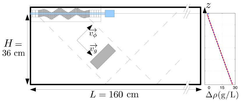
Figure 1: (color online) Sketch of the experimental setup showing the wave generator lying horizontally at the top of the wave tank. The dashed lines delimit the expected domain of propagation of the left to right propagating wave beam, once it has been emitted from the generator. For the sake of clarity, the direction of propagation of the phase and group velocities are also indicated. The tilted grey rectangle corresponds to the analysis area for the time-frequency study of section 4.2. The plot on the right shows the experimentally measured modification of the density due to salt, $\Delta\rho=\rho-1000$, as a function of the water depth $z$. Points correspond to experimental measurements while the straight line is a linear fit.

The motion of the fluid is captured by the synthetic schlieren technique using a dotted image behind the tank (Dalziel et al., 2000). A camera is used to acquire images of this background at $1.875$ frames per second. The CIVx algorithm (Fincham & Delerce, 2000) computes the cross-correlation between the real-time and the $t=0$ background images, when the fluid is at rest. This algorithm gives the variation of the horizontal, $\tilde{\rho}_{x}(x,z,t)=\partial_{x}(\rho(x,z,t)-\rho_{0}(z))$, and vertical, $\tilde{\rho}_{z}(x,z,t)=\partial_{z}(\rho(x,z,t)-\rho_{0}(z))$, density gradients, where $\rho(x,z,t)$ and $\rho_{0}(z)$ are the instantaneous and initial fluid densities.

2.2 Direct observation

In an experimental configuration where the tank is filled with a linear stratification producing a buoyancy frequency $N=0.91$ rad/s, a plane wave is generated at a frequency $\omega_{0}/N=0.74$, with an amplitude of the plates motion of $a=0.5$ cm. Figure 2(a) shows a snapshot of the density gradient field, obtained 10 oscillating periods after the wave generator was started. One can observe a plane wave extending over two wavelengths, propagating from the top left corner to the bottom right corner of the field of view, while the phase propagates from bottom left to top right. Note that the wave has reached a steady state in the visualization window. Forty oscillating periods later, a strong perturbation of the plane wave can be observed, as shown in Fig. 2(b) (see the movie in the online supplementary material). Smaller scale patterns have formed over the whole area that was initially occupied by the plane wave beam; interestingly, these patterns extend even slightly outside of this area, in the top left corner.

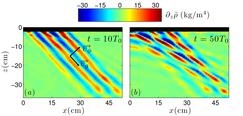
Figure 2: (color online) Snapshots of the vertical density gradient field for $t=10T_{0}$ (a) and $t=50T_{0}$ (b) where $T_{0}=2\pi/\omega_{0}$ is the primary wave period. The wave is propagating from left to right. On the left panel, the direction of the phase velocity $\overrightarrow{v_{\phi}}$ and the group velocity $\overrightarrow{v_{\rm g}}$ are indicated. Note that the shade scale (color scale online) is the same in both panels. buoyancy frequency is $N=0.91$ rad/s, the wave frequency is $\omega_{0}/N=0.74$ and the motion amplitude of the plates of the generator is $0.5$ cm.

2.3 Analysis

The measured density gradient fields are analyzed using a time-frequency representation (Flandrin, 1999) calculated at each spatial point

$$S_{r}(\omega,t)=\left<\left|\int_{-\infty}^{+\infty}{\rm d}u\,\tilde{\rho}_{r}(u)\,e^{i\omega u}\,h(t-u)\right|^{2}\right>_{xz}\,,$$ (1)

where $r$ stands for $x$ or $z$ and $h$ is a smoothing Hamming window of energy unity. A large (resp. small) window provides good frequency (resp. time) resolution. To increase the signal to noise ratio, the data is averaged on the entire area of observation. In the following, we will consider only the analysis of the vertical density gradient field, but the results are similar for the horizontal one.

Figure 3(a) shows the time-frequency spectrum for the experiment corresponding to the snapshots presented in Fig. 2. One can clearly observe that initially, only the frequency $\omega_{0}/N=0.74$ is present: it corresponds to the wave produced by the generator, which we will call the primary wave. After about 10 oscillation periods, one notices the growth of two secondary waves, with the frequencies $\omega_{1}/N=0.50$ and $\omega_{2}/N=0.24$. In order to allow a better observation of these three frequencies, we present on Fig. 3(b) a vertical cut of the time-frequency spectrum at time $t/T_{0}=50$. As can be noticed, the frequencies satisfy the condition $\omega_{1}+\omega_{2}=\omega_{0}$. We will come back to this feature in the following sections. It is interesting to notice that although the two secondary frequencies seem to shift slightly in the long time range, the resonance condition prevails. In addition, the amplitude of the two secondary waves seems to decrease after some time. Two other frequencies, $\omega/N=0$ and $\omega/N=0.98$, have non vanishing contributions to the signal. The first one corresponds to the mean flow generated by the plates of the wave generator via an Archimedes’ screw type of entrainment. A second possible source of mean flow could be the reflection of the primary wave at the bottom of the tank. The other additional frequency, $\omega/N=0.98$, can be attributed to the non-linear interaction between the waves with frequencies $\omega_{2}/N=0.24$ and $\omega_{0}/N$=0.74.

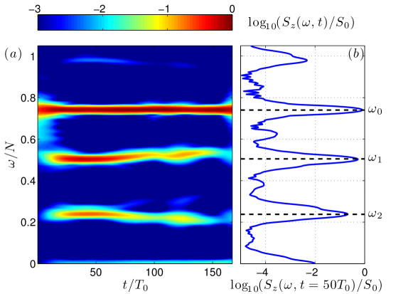
Figure 3: (color online) (a) Time frequency spectrum $S_{z}(\omega,t)$ of the gradient density field. (b) Frequency spectrum $S_{z}(\omega,t=50T_{0})$. The quantity $S_{0}$ is defined as the time average of the main component $S_{0}=\langle S_{z}(\omega_{0},t)\rangle_{t}$.

To extract more information on the various waves involved in this flow, one can filter the density gradient field around the three measured frequencies $\omega_{0}$, $\omega_{1}$ and $\omega_{2}$. This filtering operation is performed using the Hilbert transform method that was developed in Mercier et al. (2008). This method consists in a first demodulation step with a Fourier transform in time, a time filtering around the desired frequency and then returning to real space by an inverse Fourier transform. In a second step, the signal is filtered in space, allowing separation of the waves corresponding to the four possible propagation directions for a given frequency. The result of this operation applied to our measured density fields is shown in Fig. 4. The filtered density gradient fields associated with each frequency are shown in the top row, at a fixed time. Note that for the three different cases, we have kept only one quarter of the possible wavevectors as shown in the sketches of Fig. 4. Phase and group velocities being orthogonal, the propagation direction is deduced by a rotation of 90^∘, the sense of rotation being chosen to have the vertical components of the phase and group velocities of opposite signs. For the left and center columns, it corresponds to a propagation from the the top left corner to the bottom right one, while for the right column the wave beam goes from the bottom right corner to the top left one. One can clearly observe that the filtering operation extracted three distinct waves, each associated with its corresponding propagation angle. As mentioned, the Hilbert transform allows identification of the orientation of the propagation of each wave, showing that the wave at frequency $\omega_{2}$ propagates from right to left, contrary to the two others. This explains why we observe signal outside the primary wave beam in the top left corner of Fig. 2(b), as mentioned in the previous section.

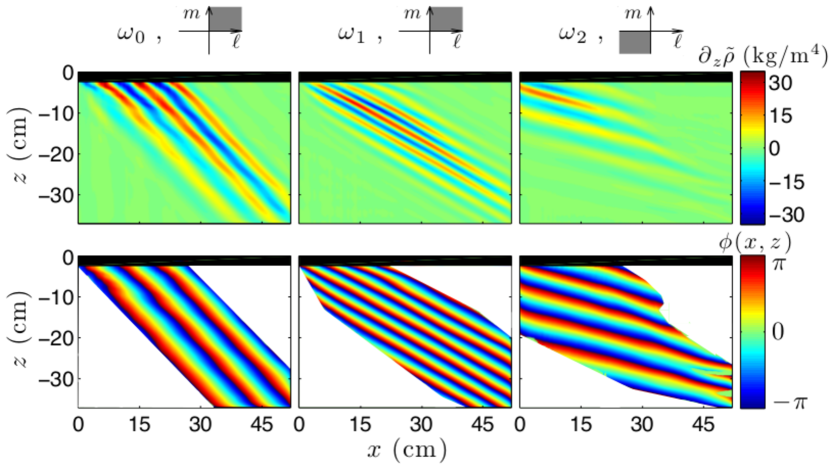
Figure 4: (color online) Top row: primary (left) and two secondary waves (center and right) obtained by applying the Hilbert spatial and temporal filtering to the density gradient field at $t/T_{0}=50$. The sketches on top indicate the domain of wavevector $(\ell,m)$ which are kept during the spatial Hilbert filtering for each column. Bottom row, corresponding phases associated to each frequency. The phase is displayed only where the wave amplitude is larger than 3% of the maximum. The experimental parameters are $N=0.91$, $\omega_{0}=0.74\ N$ and $a=0.5$ cm.

This procedure also allows extraction of the phase $\phi_{i}$ of the signal at a given frequency, $\phi_{i}(t,x,z)=\omega_{i}t\pm\ell_{i}x\pm m_{i}z$, where $(\ell_{i},m_{i})$ are the horizontal and vertical components of the wavevector $\vec{k}_{i}$. This is shown at $t=50~{}T_{0}$ in the bottom row of Fig. 4. Again, one can clearly observe a pattern of stripes parallel to the direction of propagation of each wave, corresponding to a phase propagating in the perpendicular direction. At a fixed time and $x$ (respectively $z$), the phase is linear with the position $z$ (resp. $x$). The components $\ell_{i}$ and $m_{i}$ of the wave vectors for each wave can then be obtained by differentiating $\phi_{i}(t,x,z)$ with respect to $z$ (resp. $x$). For the experiment presented in Fig. 2, one obtains $(\ell_{1}+\ell_{2})/\ell_{0}=0.89~{}\pm~{}0.17$ and $(m_{1}+m_{2})/m_{0}=0.99~{}\pm~{}0.07$. It is striking that the three vectors also satisfy a resonance condition: $\overrightarrow{k_{0}}=\overrightarrow{k_{1}}+\overrightarrow{k_{2}}$ within the experimental uncertainties. Note that the larger error on the measurement of $\ell$, compared to $m$, is related to the fact that the secondary waves are rather horizontal. Consequently the horizontal projection of the wave beam, for $\omega_{2}$, gives us only one or two horizontal wavelengths. It yields a poorer measurement of the horizontal component of their wavevector.

As a conclusion of this first set of experimental observations, we can say that the two secondary waves that are generated from the primary wave are the result of a resonant triad interaction. We will therefore study analytically in the next section the conditions under which such a triad interaction can develop.

3 Parametric subharmonic instability theory

3.1 Derivation of the equations

The two-dimensional dynamics (in the $x,z$ coordinates) of a Boussinesq fluid is usually described by the following two equations

$$\frac{\partial b}{\partial t}+J(b,\psi) = -N^{2}\frac{\partial\psi}{\partial x}\,,$$ (2)

$$\frac{\partial\nabla^{2}\psi}{\partial t}+J(\nabla^{2}\psi,\psi) = \frac{\partial b}{\partial x}+\nu\Delta^{2}\psi\,,$$ (3)

where $\psi$ is the streamfunction, while $b\equiv g\rho/\bar{\rho}$ is the buoyancy perturbation and $J$ the jacobian term defined as $J(f_{1},f_{2})=\partial_{x}f_{1}\partial_{z}f_{2}-\partial_{z}f_{1}\partial_{x}f_{2}$. The velocity field is expressed as $\overrightarrow{v}=(-\partial_{z}\psi,0,\partial_{x}\psi)$.

We seek solutions of the form

$$b = \sum_{j=0}^{2}R_{j}(t)e^{i(\vec{k}_{j}\cdot\vec{r}-\omega_{j}t)}+c.c.\,,$$ (4)

$$\psi = \sum_{j=0}^{2}\Psi_{j}(t)e^{i(\vec{k}_{j}\cdot\vec{r}-\omega_{j}t)}+c.c.\,.$$ (5)

Introducing these solutions into Eq. (2) and Eq. (3), one gets

$$\sum_{j=0}^{2}[\dot{R}_{j}-i\omega_{j}R_{j}+iN^{2}\ell_{j}\Psi_{j}]e^{i(\vec{k}_{j}\cdot\vec{r}-\omega_{j}t)}+c.c. = -J(b,\psi)\,,$$ (6)

$$\sum_{j=0}^{2}[-\kappa_{j}^{2}(\dot{\Psi}_{j}-i\omega_{j}\Psi_{j})-i\ell_{j}R_{j}-\nu\kappa_{j}^{4}\Psi_{j}]e^{i(\vec{k}_{j}\cdot\vec{r}-\omega_{j}t)}+c.c. = -J(\nabla^{2}\psi,\psi)\,,$$ (7)

if $\dot{R}$ denotes the derivative of the amplitude $R$.

The usual inviscid linear dynamics of (6) provides the polarization expression

$$R_{j}=\frac{N^{2}\ell_{j}}{\omega_{j}}\Psi_{j}\quad\textrm{for}\quad j\,=\,0,\,1\;\textrm{or}\;2\,$$ (8)

with the dispersion relation

$$\omega_{j}=s_{j}N|\ell_{j}|/\sqrt{\ell_{j}^{2}+m_{j}^{2}}$$ (9)

where $s_{j}=\pm 1$ defines the sign of the wave $j$. However, the linear system is forced on the right-hand side of Eqs. (6) and (7). After some manipulations, the Jacobian terms can be written as

$$J(b,\psi) = \sum_{p=0}^{2}\sum_{q\neq p}[(-\ell_{p}m_{q}+m_{p}\ell_{q})R_{p}\Psi_{q}]e^{i[(\vec{k}_{p}+\vec{k}_{q})\cdot\vec{r}-(\omega_{p}+\omega_{q})t]}$$ (10)

$$\qquad-[(-\ell_{p}m_{q}+m_{p}\ell_{q})R_{p}\Psi_{q}^{*}]e^{i[(\vec{k}_{p}-\vec{k}_{q})\cdot\vec{r}-(\omega_{p}-\omega_{q})t]}+c.c.\,,$$

$$J(\nabla^{2}\psi,\psi) = \sum_{p=0}^{2}\sum_{q\neq p}[(\ell_{p}m_{q}-m_{p}\ell_{q})\kappa_{p}^{2}\Psi_{p}\Psi_{q}]e^{i[(\vec{k}_{p}+\vec{k}_{q})\cdot\vec{r}-(\omega_{p}+\omega_{q})t]}$$ (11)

$$\qquad-[(\ell_{p}m_{q}-m_{p}\ell_{q})\kappa_{p}^{2}\Psi_{p}\Psi_{q}^{*}]e^{i[(\vec{k}_{p}-\vec{k}_{q})\cdot\vec{r}-(\omega_{p}-\omega_{q})t]}+c.c.\,.$$

We obtain now the evolution of a particular wavenumber component ($\vec{k}_{r},\omega_{r}$) associated with the stream function $\Psi_{r}$, in which $r=0,1$ or $2$, by averaging both the left hand side and the right hand side over the period of that wave. The resonant terms on the right hand side that will balance the left hand side will be the waves fulfilling two conditions: a spatial resonance condition

$$\vec{k}_{0}=\vec{k}_{1}+\vec{k}_{2}$$ (12)

and a temporal resonance one

$$\omega_{0}=\omega_{1}+\omega_{2}\,.$$ (13)

Collecting resonant terms and using the polarization expression (8), the Jacobian term (10) can then be written as

$$J(b,\psi) = -(\ell_{1}m_{2}-m_{1}\ell_{2})N^{2}\left(\frac{\ell_{1}}{\omega_{1}}-\frac{\ell_{2}}{\omega_{2}}\right)\Psi_{1}\Psi_{2}e^{i(\vec{k}_{0}\cdot\vec{r}-\omega_{0}t)}$$ (14)

$$+(\ell_{0}m_{2}-m_{0}\ell_{2})N^{2}\left(\frac{\ell_{0}}{\omega_{0}}-\frac{\ell_{2}}{\omega_{2}}\right)\Psi_{0}\Psi_{2}^{*}e^{i(\vec{k}_{1}\cdot\vec{r}-\omega_{1}t)}$$

$$+(\ell_{0}m_{1}-m_{0}\ell_{1})N^{2}\left(\frac{\ell_{0}}{\omega_{0}}-\frac{\ell_{1}}{\omega_{1}}\right)\Psi_{0}\Psi_{1}^{*}e^{i(\vec{k}_{2}\cdot\vec{r}-\omega_{2}t)}$$

$$+\mbox{NRT}\,,$$

where NRT stands for non resonant terms that are not important in the problem. In the same way, one gets the Jacobian term (11)

$$J(\nabla^{2}\psi,\psi) = \ \ (\ell_{1}m_{2}-m_{1}\ell_{2})(\kappa_{1}^{2}-\kappa_{2}^{2})\Psi_{1}\Psi_{2}e^{i(\vec{k}_{0}\cdot\vec{r}-\omega_{0}t)}$$ (15)

$$-(\ell_{0}m_{2}-m_{0}\ell_{2})(\kappa_{0}^{2}-\kappa_{2}^{2})\Psi_{0}\Psi_{2}^{*}e^{i(\vec{k}_{1}\cdot\vec{r}-\omega_{1}t)}$$

$$-(\ell_{0}m_{1}-m_{0}\ell_{1})(\kappa_{0}^{2}-\kappa_{1}^{2})\Psi_{0}\Psi_{1}^{*}e^{i(\vec{k}_{2}\cdot\vec{r}-\omega_{2}t)}$$

$$+\mbox{NRT}\,.$$

Introducing this result into equation (7), one obtains the three following relations between $\Psi_{r}$ and $R_{r}$ for each individual phase $\exp[{i(\vec{k}_{r}\cdot\vec{r}-\omega_{r}t)}]$ in which $r=0,1$ or $2$

$$R_{0} = \frac{i}{\ell_{0}}\left[\kappa_{0}^{2}(\dot{\Psi}_{0}-i\omega_{0}\Psi_{0})+\nu\kappa_{0}^{4}\Psi_{0}-\gamma_{0}\alpha_{0}\Psi_{1}\Psi_{2}\right]\,,$$ (16)

$$R_{1} = \frac{i}{\ell_{1}}\left[\kappa_{1}^{2}(\dot{\Psi}_{1}-i\omega_{1}\Psi_{1})+\nu\kappa_{1}^{4}\Psi_{1}-\gamma_{1}\alpha_{1}\Psi_{0}\Psi^{*}_{2}\right]\,,$$ (17)

$$R_{2} = \frac{i}{\ell_{2}}\left[\kappa_{2}^{2}(\dot{\Psi}_{2}-i\omega_{2}\Psi_{2})+\nu\kappa_{2}^{4}\Psi_{2}-\gamma_{2}\alpha_{2}\Psi_{0}\Psi^{*}_{1}\right]\,,$$ (18)

where $\gamma_{0}=+1$, $\gamma_{1,2}=-1$ and $\alpha_{r}=(\ell_{p}m_{q}-m_{p}\ell_{q})(\kappa_{p}^{2}-\kappa_{q}^{2})\,,$ in which $p,q,r=0,1,2$ or any circular permutation.

3.2 Slow amplitude variation

Experimental results have strongly suggested that the amplitude of $\Psi$ varies slowly with respect to the period of the primary wave. It is therefore appropriate to consider $\dot{\Psi}_{j}\ll i\omega_{j}\Psi_{j}$ so that differentiating (8) leads to

$$\dot{R}_{j}\approx\frac{\omega_{j}}{\ell_{j}}\kappa_{j}^{2}\dot{\Psi}_{j}\,.$$ (19)

One gets for Eq. (6)

$$\frac{i}{\ell_{0}}\left[(N^{2}\ell_{0}^{2}-\omega_{0}^{2}\kappa_{0}^{2})\Psi_{0}\right. - \left.2i\omega_{0}\kappa_{0}^{2}\dot{\Psi}_{0}-i\omega_{0}\nu\kappa_{0}^{4}\Psi_{0}+i\omega_{0}s_{0}\alpha_{0}(\Psi_{1}\Psi_{2})\right]$$ (20)

$$= (\ell_{1}m_{2}-m_{1}\ell_{2})N^{2}\left(\frac{\ell_{1}}{\omega_{1}}-\frac{\ell_{2}}{\omega_{2}}\right)\Psi_{1}\Psi_{2}\,,$$

$$\frac{i}{\ell_{r}}\left[(N^{2}\ell_{r}^{2}-\omega_{r}^{2}\kappa_{r}^{2})\Psi_{r}\right. - \left.2i\omega_{r}\kappa_{r}^{2}\dot{\Psi}_{r}-i\omega_{r}\nu\kappa_{r}^{4}\Psi_{r}+i\omega_{r}s_{r}\alpha_{r}(\Psi_{0}\Psi_{p}^{*})\right]$$ (21)

$$= -(\ell_{0}m_{p}-m_{0}\ell_{p})N^{2}\left(\frac{\ell_{0}}{\omega_{0}}-\frac{\ell_{p}}{\omega_{p}}\right)\Psi_{0}\Psi_{p}^{*}\,.$$

Each wave satisfies the dispersion relation, $N^{2}\ell_{r}^{2}=\omega_{r}^{2}\kappa_{r}^{2}$. After some calculations, one gets

$$2i\omega_{0}\kappa_{0}^{2}\dot{\Psi}_{0}=\left[i\omega_{0}s_{0}\alpha_{0}-\frac{\ell_{0}}{i}(\ell_{1}m_{2}-m_{1}\ell_{2})N^{2}\left(\frac{\ell_{1}}{\omega_{1}}-\frac{\ell_{2}}{\omega_{2}}\right)\right]\Psi_{1}\Psi_{2}-i\omega_{0}\nu\kappa_{0}^{4}\Psi_{0}$$ (22)

$$=i(\ell_{1}m_{2}-m_{1}\ell_{2})\left[s_{0}\omega_{0}(\kappa_{1}^{2}-\kappa_{2}^{2})+\ell_{0}N^{2}\left(\frac{\ell_{1}}{\omega_{1}}-\frac{\ell_{2}}{\omega_{2}}\right)\right]\Psi_{1}\Psi_{2}-i\omega_{0}\nu\kappa_{0}^{4}\Psi_{0}\,,$$ (23)

which can be simplified as

$$\dot{\Psi}_{0}=I_{0}\Psi_{1}\Psi_{2}-\frac{\nu}{2}\kappa_{0}^{2}\Psi_{0}.$$ (24)

Similar calculations for waves $1$ and $2$ lead to

$$\dot{\Psi}_{1}=-I_{1}\Psi_{0}\Psi_{2}^{*}-\frac{\nu}{2}\kappa_{1}^{2}\Psi_{1}\,,$$ (25)

$$\dot{\Psi}_{2}=-I_{2}\Psi_{0}\Psi_{1}^{*}-\frac{\nu}{2}\kappa_{2}^{2}\Psi_{2}\,,$$ (26)

where

$$I_{r}=\frac{\ell_{p}m_{q}-m_{p}\ell_{q}}{2\omega_{r}\kappa_{r}^{2}}\left[\omega_{r}(\kappa_{p}^{2}-\kappa_{q}^{2})+l_{r}N^{2}\left(\frac{\ell_{p}}{\omega_{p}}-\frac{\ell_{q}}{\omega_{q}}\right)\right].$$ (27)

3.3 Solution

We consider that $\Psi_{0}$ corresponds to the primary wave and is constant in early times since amplitudes of the secondary waves, $\Psi_{1}$ and $\Psi_{2}$ are negligible with respect to $\Psi_{0}$. One can combine equations (25) and (26) to get

$${\ddot{\Psi}_{1}}=I_{1}I_{2}\Psi_{0}^{2}\Psi_{1}-\frac{\nu^{2}}{4}\kappa_{2}^{2}\kappa_{1}^{2}\Psi_{1}-\frac{\nu}{2}(\kappa_{1}^{2}+\kappa_{2}^{2}){\dot{\Psi}_{1}}\,.$$ (28)

The solution of Eq. (28) leads to the expression $\Psi_{1,2}(T)=A_{1,2}\,e^{\sigma_{+}T}+B_{1,2}e^{\sigma_{-}T},$ by introducing the growth rate

$$\sigma_{\pm}=-\frac{\nu}{4}(\kappa_{1}^{2}+\kappa_{2}^{2})\pm\sqrt{\frac{\nu^{2}}{16}(\kappa_{1}^{2}-\kappa_{2}^{2})^{2}+I_{1}I_{2}|\Psi_{0}|^{2}}.\quad$$ (29)

A vanishingly small amplitude noise induces the growth of two secondary waves. In conclusion, a primary plane wave can be unstable by a parametric subharmonic mechanism. The growth rate of the instability is not only function of the characteristics of the primary wave, namely its wavevector and its frequency through the coefficients $I_{1}$ and $I_{2}$, but also its amplitude $\Psi_{0}$ and the viscosity $\nu$.

3.4 Resonance loci and growth rates

In the following, we consider that only the primary wave $\Psi_{0}$, of given frequency $\omega_{0}$, wavevector $\overrightarrow{k_{0}}$ = $(\ell_{0},m_{0})$ and sign $s_{0}$, is present initially in the system, while $\Psi_{1,2}$ is experimentally only present as the noise. Without loss of generality, we can choose $s_{0}=+1$ (which is given by the experimental configuration, or more precisely by the direction of rotation of the cams). The two secondary waves ($s_{1}$, $\omega_{1}$, $\overrightarrow{k_{1}}$) and ($s_{2}$, $\omega_{2}$, $\overrightarrow{k_{2}}$) which could form a resonant triad with the primary wave have to be determined using the resonance conditions (12) and (13). From the dispersion relation for internal waves (9), the resonance conditions lead to

$$s_{0}\frac{|\ell_{0}|}{\sqrt{\ell_{0}^{2}+m_{0}^{2}}} = s_{1}\frac{|\ell_{1}|}{\sqrt{\ell_{1}^{2}+m_{1}^{2}}}+s_{2}\frac{|\ell_{0}+\ell_{1}|}{\sqrt{(\ell_{0}+\ell_{1})^{2}+(m_{0}+m_{1})^{2}}}\,.$$ (30)

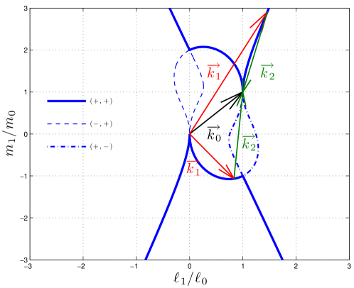
Figure 5: (color online) The curves represent the location of $(\ell_{1},m_{1})$ satisfying Eq. (30) for the three possible combinations of signs, once the wavevector $\overrightarrow{k_{0}}=(\ell_{0},m_{0})$ of the primary wave is given. The curves are represented by solid lines when the growth rates have a positive real part, while the dashed lines corresponds to the neutrally stable cases, for which the real part of the growth rate is always zero in a non viscous case and negative when viscosity sets in. Two examples of vector triads ($\overrightarrow{k_{0}}$, $\overrightarrow{k_{1}}$,$\overrightarrow{k_{2}}$) are shown.

For a given primary wave $(s_{0},\ell_{0},m_{0})$, the solution of this equation for each sign combination $(s_{0},s_{1},s_{2})$ is a curve in the $(\ell_{1},m_{1})$ plane which is presented in Fig. 5. Since $s_{0}=+1$, it is then necessary to consider four sign combinations for $(s_{1},s_{2})$: $(-,-)$, $(+,-)$, $(-,+)$ and $(+,+)$. However, there is no solution of equation (30) in the $(-,-)$ case. In addition, the combinations $(+,-)$ and $(-,+)$ are neutrally stable, i.e. the real part of $\sigma$ is always zero in a non viscous case and negative when viscosity sets in. For this reason, in what follows, we will focus only on the $(+,+)$ combination.

In Fig. 5, any point of the solid curve corresponds to the tip of the $\overrightarrow{k_{1}}$ vector, wich satisfy the equation 30 with $s_{0}=s_{1}=s_{2}=+1$. We obtain also $\overrightarrow{k_{2}}$ by construction, closing the triangle. Two examples are illustrated with solid arrows. However, to predict which is the one expected to be seen experimentally, one has to determine the largest growth rate. For a given sign of $m_{1}$, three distinct parts of the $(+,+)$ curves can be observed in Fig. 5, corresponding to $\ell_{1}/\ell_{0}>1$, $\ell_{1}/\ell_{0}<0$ and $0<\ell_{1}/\ell_{0}<1$. It will prove convenient in what follows to separate the study in these three regions, in order to evidence the direction of energy transfer (towards smaller scales or larger scales).

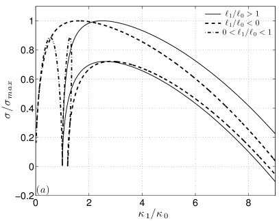
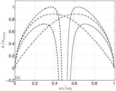
Figure 6: (color online) Growth rates $\sigma$ computed from Eq. (29), as a function of the wave vector modulus $\kappa_{1}$ in panel (a) and as a function of the wave frequency $\omega_{1}$ in panel (b). The three possible sign combinations have been superimposed. The primary wave vector $\vec{k}_{0}$ is chosen arbitrarily, as well as its amplitude, which value, normalized by the viscosity, is $\Psi_{0}/\nu=100$. $\kappa_{0}$ and $\omega_{0}$ are respectively the wave vector modulus and the frequency of the primary wave.

In Fig. 6, the predicted growth rates $\sigma$ are plotted as a function of $\kappa_{1}/\kappa_{0}$ and $\omega_{1}/\omega_{0}$ only for the (+,+) combination, with distinct line types for the different regions defined above. There are two curves for each line type, corresponding to different signs of $m_{1}$ (top half and bottom half in Fig. 5).

One can notice that in both plots, the solid curve ($\ell_{1}/\ell_{0}>1$) and the dashed curve ($\ell_{1}/\ell_{0}<0$) reach the same maximum value. Moreover, one can observe in Fig. 6(b) that the maximum are obtained for $\omega_{1}=0.37\ \omega_{0}$ (dashed curve) and for $\omega_{1}=0.63\ \omega_{0}$ (solid curve), two frequencies which sum is equal to $\omega_{0}$. More generally, Fig. 6(b) shows that the solid and dashed curves are mutually symmetric with respect to the central value $\omega/\omega_{0}=0.5$. It shows that if $\overrightarrow{k_{1}}$ is selected on the solid curve, $\overrightarrow{k_{2}}$ will be selected on the dashed curve and conversely. In an arbitrary way, we will always take $\overrightarrow{k_{1}}$ on the solid curve (largest wavenumber) and consequently $\overrightarrow{k_{2}}$ will be determined by the dashed curve (lowest wavenumber among the secondary waves).

As to the dotted dashed curve, one can notice that it has two maxima. The two secondary wave vectors are, in this case, selected in the same area ($0<\ell_{1}/\ell_{0}<1$). For all the curves, one notices that the growth rates become negative when $\kappa_{1}\rightarrow\infty$ (because of viscosity).

Interestingly, the growth rate is positive for a broad range of wavenumbers and it is rather flat on the maximum, emphasizing that the parametric resonance is weakly selective in this regime. The values of $\kappa_{1}$ corresponding to significant growth rates are of the same order of magnitude as the primary wavenumber $\kappa_{0}$, indicating that the viscosity has a significant effect on the selection of the excited resonant triad, preventing any large wave number secondary wave to grow from the instability. For the frequency value considered, the maximum growth rate is obtained for $\kappa_{1}=2.5\ \kappa_{0}$ and $\kappa_{2}=1.62\ \kappa_{0}$.

4 Comparison with the experiment

4.1 Wave vectors

In section 2, we observed that the experimental values of frequencies and wave vectors satisfy the conditions of temporal and spatial resonance (12) and (13). The theoretical derivation gives us the dependence of the growth rate with the wave vector of one of the secondary waves (the second wave is then defined by the resonance condition). We can now check if the observed wave vectors correspond to the largest growth rates, as could be expected. For pedagogical reasons, the value of $\Psi_{0}$ used to compute the plots in section 3 was arbitrarily chosen to enhance the case (external branches of the resonance loci) where the energy transfer goes from large scales to smaller scales. The vector $\overrightarrow{k_{0}}$ was also chosen arbitrarily. In this section, we will use the experimental values for $\overrightarrow{k_{0}}$ as well as for the amplitude $\Psi_{0}$. This last quantity is measured using the modulus of the Hilbert Transform of the density gradient field for the primary wave, calculated in the same area used for the measurement of the growth rate. Figure 7(a) shows the theoretical resonance loci (blue curve) computed identically to the one in Fig. 5, but using the experimental $\overrightarrow{k_{0}}$. The three arrows correspond to the experimental measurement of the three wave vectors. As mentioned in section 2, it can be observed that the spatial resonance condition is satisfied. Figure 7(b) represents the evolution of the growth rate with $\kappa_{1}$. Comparing Fig. 6(a) and  7(b), is interesting to note that the reduction of the primary wave amplitude by a factor of 4 results in an enhancement of the ($0<\ell_{1}/\ell_{0}<1$) type of instability, with respect to the ($\ell_{1}/\ell_{0}>1$) type.

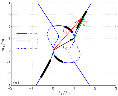
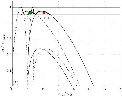
Figure 7: (color online) (a) The solid blue curve represents the resonance loci for the secondary wave vector $\overrightarrow{k_{1}}$, in the case where the primary wave vector $\overrightarrow{k_{0}}$ corresponds to the experiment presented in § 2, i.e. $\ell_{0}=66\pm 2$ m^-1, $m_{0}=59$ $\pm 2$ m^-1 and $\omega_{0}/N=0.74$. The three arrows represent the experimental measurement of the three wave vectors $\overrightarrow{k_{0}}$ (black), $\overrightarrow{k_{1}}$ (red) and $\overrightarrow{k_{2}}$ (green). (b) Growth rates $\sigma$ computed from Eq. (29), as a function of the wave vector modulus, in the case where the primary wave vector $\overrightarrow{k_{0}}$ corresponds to the experiment presented in section 2, as well as the primary wave amplitude ($\Psi_{0}/\nu=28$). The two horizontal lines mark the maximum growth rate and 90% of the maximum. The thick lines on the left panel show the regions corresponding to a growth rate belonging to this interval. The experimentally measured growth rate are shown for the observed wavenumber $\kappa_{1}$ (red square) and $\kappa_{2}$ (green circle). The experimental error bars on the growth rate measurement beeing large (of the order of 25%, see text), they are not represented for these two points, for the sake of clarity.

According to the theory, the secondary waves generated by the instability should be the ones corresponding to the largest growth rate. However, an instability is initially generated via a very small amplitude noise and because of the specific experimental conditions, not all temporal and spatial frequencies will be present in this noise with the same amplitude. In addition, as can be seen in Fig. 7(b), the growth rate curve in the case of the ($0<\ell_{1}/\ell_{0}<1$) type of instability, although it has a slightly higher maximum, is much less broad than the curve for the other type, therefore showing a very strong wavenumber sensitivity. For these reasons, we will introduce a less constrained selection criteria by allowing the unstable wave vectors to be associated with a growth rate belonging to an interval between $90\%$ and $100\%$ of the maximum growth rate. This selection criteria is illustrated in Fig. 7 (b) by thicker line and the loci for the corresponding wave vectors are represented in Fig. 7 (a) by thick black segments. It is interesting to note that this procedure allows a selection of wave vectors in different regions of the resonance loci curve. The measured wave vectors, within their experimental error, fall on one pair of these selected regions, namely on the external branches of the resonance loci. This selection corresponds, as mentioned earlier, to a slightly lower growth rate than the maximum, but to a broader curve.

4.2 Growth rates

We will now compare the experimental and theoretical values of the growth rate. The experimental determination of the growth rate $\sigma$ is obtained by calculating a time-frequency spectrum of an area taken inside the primary wave beam, as defined in Fig. 1 by the grey area. Then, the time evolution of each partial component frequency is plotted. Figure 8 shows this evolution for the same experimental run used in § 2. The growth rate is then defined as the slope of the growth region. It must be noted that the amplitude of the primary plane wave is not constant on the entire beam because of the viscous damping. For this reason, the position of the area where the spectrum is computed will influence the result for the determination of $\sigma$. An estimate of the error due to this effect is therefore performed by varying this position.

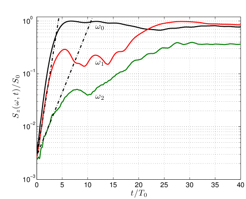
Figure 8: (color online) Amplitude of time frequency representation, $S_{z}(\omega,t)$ of the secondary wave $\omega_{1}$ and $\omega_{2}$ normalized by the amplitude of the primary wave. The dashed-dotted lines show the linear fit, from which the experimental value of the growth rate $\sigma$ is extracted. The quantity $S_{0}$ is defined as the time average of the main component $S_{0}=\langle S_{z}(\omega_{0},t)\rangle_{t}$.

For the theoretical evaluation of the growth rate, a necessary ingredient is the amplitude $\Psi_{0}$ of the primary wave. This amplitude cannot be obtained directly from the amplitude of oscillation of the generator plates, since there is a conversion factor between both described by Mercier et al. (2010). This factor is not well known, and strongly depends on the wave frequency, because of the change of angle it implies of the wave propagation, while the generator motion is only vertical. For this reason, $\Psi_{0}$ has to be measured experimentally, introducing an experimental error in the prediction. It leads to a theoretical prediction for the growth rate $\sigma=0.087~{}\pm~{}0.005$ s^-1, while the experimental measurement gives $\sigma=0.08\pm 0.02$ s^-1. The agreement between theory and experiment is rather good.

5 Dependence with primary wave frequency and amplitude

So far the experimental results shown correspond to a given amplitude, frequency and wave vector for the primary wave. It seems appropriate to study the effect of a variation of these parameters.

First, we have observed, based on the theoretical study, that the value of $\kappa_{0}$ has no effect on the selection of the secondary waves. It leaves unchanged the shape of the growth rate evolution with $\kappa_{1}$ and $\omega_{1}$ (Fig. 6). The only effect of an increase of $\kappa_{0}$ is an increase of the overall value of the growth rate. For this reason, it was not necessary to perform a systematic experimental study of the dependence of the growth rate with $\kappa_{0}$.

In a first part, we will discuss the dependence with the primary wave frequency $\omega_{0}$. Figure 9 shows the evolution with $\omega_{0}/N$ of the (normalized) norms $\kappa_{1}$ and $\kappa_{2}$ of the secondary waves corresponding to the maximum growth rate. One pair of curves (solid lines) corresponds to wave vectors on the external branches of the resonance loci and the other pair (dashed-dotted lines) to wave vectors on the central part of the resonance loci. These curves are obtained in the case where the primary wave amplitude is fixed at the value of the experimental run described in section 2. We can observe that in this case, when the secondary wave vectors belong to the external branches, there exist a range of frequency (for $\omega_{0}/N>0.78$) where the secondary wavelengths are both smaller than the primary wavelength, corresponding to an energy transfer to smaller scales. On the contrary, when the secondary wave vectors belong to the central part of the resonance loci (dashed-dotted lines), one of the secondary wavelengths is always larger than the primary wavelength, while the other is smaller, allowing for energy transfer to both smaller and larger scales.

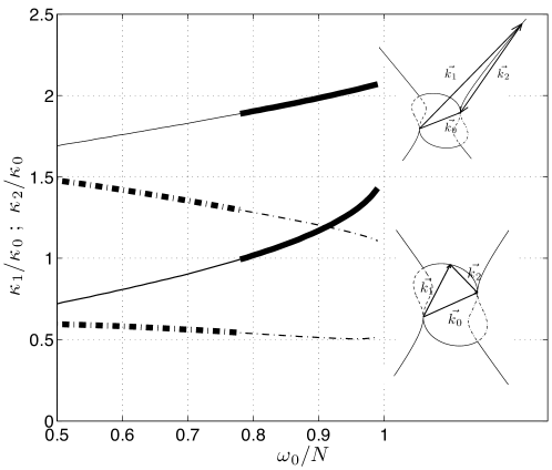
Figure 9: Evolution of $\kappa_{1}/\kappa_{0}$ and $\kappa_{2}/\kappa_{0}$ with the pulsation $\omega_{0}$ for a fixed amplitude. Solid curve: Configuration where the triad is formed on the external branches of the resonance loci (see illustration in the top inset). Dashed dotted curve: configuration where the triad is formed on the central part of the resonance loci (see illustration in the bottom inset). The thick part of curves represent the region where the growth rate is larger in this configuration, compared to the other.

Out of these two sets of secondary wave vectors, the one which corresponds to the largest growth rate is illustrated on the graph by a thicker line. There is therefore a transition frequency (in this case around $\omega_{0}/N=0.77$) for which the instability “jumps” from one solution to the other.

As mentioned, this change in behavior is observed for a given value of the amplitude $\Psi_{0}$. As this amplitude varies, the transition frequency changes. Figure 10 shows (solid line) the evolution of this transition frequency as a function of the amplitude. Above this curve, the secondary waves are selected on the outer region of the resonance loci, while below the curve the secondary waves are selected in the central zone.

On the same figure, we superimposed the experimental points obtained for different values of $\omega_{0}$ and $\Psi_{0}$, showing in which cases the parametric subharmonic instability (PSI) was observed. Three different wave generator amplitudes were used to produce these series of points (cam eccentricities of $0.1$, $0.5$ and $0.75$ cm). These three series correspond to the three almost vertical series of black symbols on the graph. One must keep in mind that the wave amplitude is computed from the measured signals, therefore a fixed amplitude of the wave generator does not correspond exactly to a fixed wave amplitude.

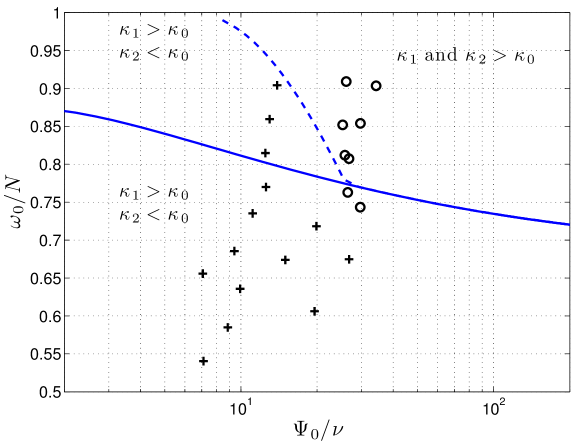
Figure 10: (color online) Phase diagram showing the dependence of the PSI instability with excitation frequency and primary wave amplitude. The solid line represents the transition between the configuration where the triad forms on the external branches of the resonance loci and the configuration where the triad is on the central part. The dashed line represents the cutoff frequency under which energy transfer to larger scales is involved in the PSI. Symbols correspond to experimental data points: ($\circ$) observed PSI, (+) no apparent PSI.

It can be noted that for large enough excitation amplitudes, PSI is observed, but mostly above the transition line. Actually, after careful observation, it turns out that the two points with PSI below this line are also case of PSI with wave vectors on the external branches of the resonance loci. This feature may be related to the uncertainty on the frequency selection mentioned in section 4.1.

Our guess is that PSI cannot develop in the present experimental tank when one of the secondary waves has a larger wavelength than the primary wave. No cascade to larger scale is allowed. The reason for this behavior could be the too small number of wavelengths which is excited by the generator.

For the smallest excitation amplitude, no PSI was observed during the recording, even for experimental runs located above the solid line of figure 10. Equation (29) shows that unstable solutions are possible only if the amplitude of the primary wave exceeds a viscous threshold value given by $2\sqrt{\nu\kappa_{1}\kappa_{2}/(I_{1}I_{2})}$. However, the excitation amplitude is one or two orders of magnitude larger than this viscous threshold which cannot explain the absence of the instability. This behavior could again be related to the size of the expected wavelengths at this amplitude. Indeed, it can be observed in Fig. 9 that the lower solid line crosses the ordinate 1 at a given frequency. This implies that, below this frequency, although the secondary waves are selected on the external branches, a transfer to larger scales is however involved. We have computed theoretically, as a function of the wave amplitude, the threshold frequency under which a transfer to larger scales is present for secondary waves selected on the external branches. It is plotted in Fig. 10 as a dashed line. The small amplitude series, where no PSI is observed, happens to be on the left of this line, therefore in the region involving transfer to larger scales. As in the case of small frequencies, this might explain the absence of observed PSI. To summarize, the only region in the phase space where no energy is transfered to larger scales is the top right corner (above the solid line and right of the dashed line) and it is the only region where we observe PSI, which seems to agree with our assumption of limitation due to the finite size of the primary wave beam.

6 Discussion

Using a synthetic schlieren technique in a linearly stratified fluid, we have observed the production, from a primary internal plane wave, of two secondary waves of smaller frequency and wavelength. The mechanism at play is a 3-wave resonant interaction, satisfying a temporal resonance condition for the three pulsations $\omega_{0}=\omega_{1}+\omega_{2}$ and a spatial resonance condition for the three wave vectors, $\overrightarrow{k_{0}}=\overrightarrow{k_{1}}+\overrightarrow{k_{2}}$. This resonant interaction can be developed analytically, in order to produce theoretical predictions that we compare to our measurements, which are derived from applying a time-frequency spectrum and a Hilbert transform to our data. A good agreement was found for the wave vectors of the secondary waves, as well as for the instability growth rate.

The relevance of PSI for oceanic internal waves has been recently renewed by several numerical simulations with realistic conditions (see for example Hibiya et al. (2002) or MacKinnon & Winters (2005)), which have been followed by very interesting field measurements which also pointed to the presence of PSI activity in the ocean. One might in particular refer to measurements close to Hawaii by Rainville & Pinkel (2006a), Carter & Gregg (2006) or Alford et al. (2007).

However, in the ocean, due to the large spatial scales, the role of viscosity is reduced compared to the experiment. In order to illustrate this point, let us consider a typical oceanic internal wave, measured in situ by observing the periodic oscillations of isotherms (see figure 1 in Cairns & Williams (1976) or figure 6.13 in Sutherland (2010)). Theses oscillations have an amplitude of about 20 m, with a period of about half a day. Ocean internal waves typically have wavelengths from hundreds of meters to tens of kilometers (Garrett & Munk, 1972; LeBlond & Mysak, 1978; Susanto et al., 2005): as a typical value, we shall take 1000 m. Compared to our experiment, it yields an amplitude of the stream function $\Psi_{0}$$/\nu$ about four orders of magnitude larger. We therefore recomputed as an example (see Fig. 11) the curves of Fig. 7(b), as well as the corresponding plots as a function of the wave frequency, for an amplitude 10000 times larger than the experiment. As can be observed in Fig. 11(a), the most unstable mode corresponds to the situation where the norm of both secondary wave vectors are much larger (10 to 20 times in our example) than the norm of the primary wave vector, leading to ${\overrightarrow{k_{1}}\simeq\overrightarrow{k_{2}}}$ and correspondingly (Fig. 11(b)) to $\omega_{1}\simeq\omega_{2}\simeq\omega_{0}/2$. This is what led historically to call this resonant interaction "Parametric subharmonic instability”, because of the similarity with parametric instability, like that occurring for a pendulum with oscillating suspension.

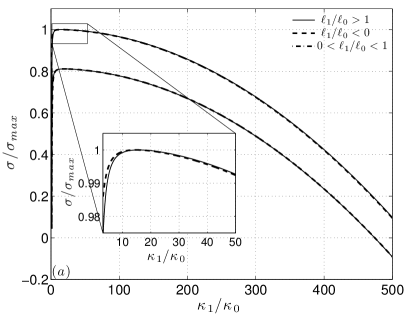
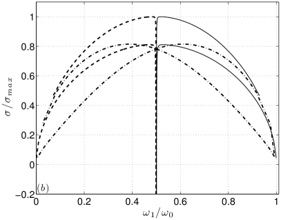
Figure 11: (color online) Growth rates $\sigma$ as a function of the wave vector modulus $\kappa_{1}$ in panel (a) and as a function of the wave frequency $\omega_{1}$ in panel (b) for typical oceanic parameters (see text).

In our experimental tank, with dimensions orders of magnitude smaller than in the ocean, we observe that viscosity has a much larger effect on the selection of the unstable modes. Indeed, because of viscosity, $\kappa_{1}$ and $\kappa_{2}$ are of the same order of magnitude as $\kappa_{0}$. In addition, a second effect of viscosity is to allow two different behaviors for the instability. First, the instability can generate two new internal waves whose wavelengths are smaller than the primary wavelength. We have then an energetic transfer to smaller scales, as is the case in the ocean. But theoretically, when $\Psi_{0}/\nu$ is small enough, the instability can also generate two secondary internal waves with one of the wavelengths larger than the primary wavelength, and the other one smaller. In this case, the energetic transfer will be to larger and smaller scales simultaneously. However, we never observed experimentally this second behavior, although it was expected from the analytical study. We observe the instability, on a plane wave, only when the theory predicts two smaller wavelengths. It is possible that the finite size of the beam impedes the development of the secondary wave, which has a larger wavelength. It could be interesting to perform some numerical simulations, with a confined beam to confirm this behavior.

Another issue that needs to be discussed is the physical location of the birth of the secondary waves. In all the experiments performed, the instability appears first in a region very close to the wave generator. This is understandable because it is the location where the primary wave first appears and where its amplitude is maximum. Then it occupies the whole volume.

In addition to the importance of the mechanism for the dissipation of waves, an effect on the background media in which waves are propagating can be expected: indeed, the primary wave could give rise through this instability to two secondary waves which are above the overturn threshold. Because of the latter, the stratification will evolve through these mixing events, influencing through this feedback effect the threshold for the mechanism itself.

Supplementary material

Supplementary materials are available at journals.cambridge.org/flm.

References

- Alford et al. (2007) Alford, M. H., MacKinnon, J. A., Zhao, Z., Pinkel, R., Klymak, J. & Peacock, T. 2007 Internal waves across the pacific. Geophysical Research Letters 34, L24601.
- Benielli & Sommeria (1998) Benielli, D. & Sommeria, J. 1998 Excitation and breaking of internal gravity waves by parametric instability. Journal of Fluid Mechanics 374, 117–144.
- Bordes et al. (2012) Bordes, G., Moisy, F., Dauxois, T. & Cortet, P. P. 2012 Experimental evidence of a triadic resonance of plane inertial waves in a rotating fluid. Physics of Fluids 24 (1), 014105.
- Bouruet-Aubertot et al. (1995) Bouruet-Aubertot, P., Sommeria, J. & Staquet, C. 1995 Breaking of standing internal gravity waves through two-dimensional instabilities. Journal of Fluid Mechanics 285, 265–301.
- Cairns & Williams (1976) Cairns, J. L. & Williams, G. O. 1976 Internal wave observations from a midwater float, part ii. Journal of Geophysical Research 81, 1943–1950.
- Carnevale et al. (2001) Carnevale, G. F., Briscolini, M. & Orlandi, P. 2001 Buoyancy- to inertial-range transition in forced stratified turbulence. Journal of Fluid Mechanics 427, 205–239.
- Carter & Gregg (2006) Carter, G & Gregg, M. 2006 Persistent near-diurnal internal waves observed above a site of m2 barotropic-to-baroclinic conversion. Journal of Physical Oceanography 36 (1136–1146.).
- Dalziel et al. (2000) Dalziel, S. B., Hughes, G. O. & Sutherland, B. R. 2000 Whole-field density measurements by ‘synthetic schlieren’. Experiments in Fluids 28 (4), 322–335.
- Dauxois & Young (1999) Dauxois, T. & Young, W. R. 1999 Near-critical reflection of internal waves. Journal of Fluid Mechanics 390, 271.
- Fincham & Delerce (2000) Fincham, A & Delerce, G 2000 Advanced optimization of correlation imaging velocimetry algorithms. Experiments in Fluids 29 (S), S13–S22, 3rd International Workshop on Particle Image Velocimetry, Santa Barbara, California, Sept. 16-18, 1999.
- Flandrin (1999) Flandrin, P. 1999 Time-Frequency/Time-Scale Analysis, Time-Frequency Toolbox for Matlab©. Academic Press, San Diego.
- Garrett & Munk (1972) Garrett, C. J. R. & Munk, W. H. 1972 Space-time scales of internal waves. Geophys. Fluid Dyn. 3, 225–264.
- Gostiaux et al. (2007) Gostiaux, L., Didelle, H., Mercier, S. & Dauxois, T. 2007 A novel internal waves generator. Experiments in Fluids 42 (1), 123–130.
- Hasselmann (1967) Hasselmann, K. 1967 A criterion for nonlinear wave stability. Journal of Fluid Mechanics 30 (04), 737–739.
- Hibiya et al. (2002) Hibiya, T, Nagasawa, M & Niwa, Y 2002 Nonlinear energy transfer within the oceanic internal wave spectrum at mid and high latitudes. Journal of Geophysical Research-Oceans 107 (C11), 3207.
- Johnston et al. (2003) Johnston, T. M. S., Merrifield, M. A. & Holloway, P. E. Internal tide scattering at the Line Islands ridge 2003 Internal tide scattering at the line islands ridge. Journal of Geophysical Research 108, 3365.
- Joubaud et al. (2012) Joubaud, S., Munroe, J., Odier, P. & Dauxois, T. 2012 Experimental parametric subharmonic instability in stratified fluids. Physics of Fluids 24 (4), 041703.
- Koudella & Staquet (2006) Koudella, C. R. & Staquet, C. 2006 Instability mechanisms of a two-dimensional progressive internal gravity wave. Journal of Fluid Mechanics 548, 165–196.
- Kunze & Smith (2004) Kunze, E. & Smith, S. G. L. 2004 The role of small-scale topography in turbulent mixing of the global ocean. Oceanography 17 (1), 55–64.
- LeBlond & Mysak (1978) LeBlond, P. H. & Mysak, L. A. 1978 Waves in the Ocean. Elsevier Sciences, New York.
- MacKinnon & Winters (2005) MacKinnon, J. A. & Winters, K.B. 2005 Subtropical catastrophe: significant loss of low-mode tidal energy at 28.9 degrees. Geophysical Research Letters 32 (15), L15605.
- McEwan (1971) McEwan, A. D. 1971 Degeneration of resonantly-excited standing internal gravity waves. Journal of Fluid Mechanics 50 (03), 431–448.
- McEwan et al. (1972) McEwan, A. D., Mander, D. W. & Smith, R. K. 1972 Forced resonant second-order interaction between damped internal waves. Journal of Fluid Mechanics 55 (04), 589–608.
- McEwan & Plumb (1977) McEwan, A. D. & Plumb, R. A. 1977 Off-resonant amplification of finite internal wave packets. Dynamics of Atmospheres and Oceans 2 (1), 83–105.
- McGoldrick (1965) McGoldrick, L. F. 1965 Resonant interactions among capillary–gravity waves. Journal of Fluid Mechanics 21 (2), 305–331.
- Mercier et al. (2008) Mercier, M. J., Garnier, N. B. & Dauxois, T. 2008 Reflection and diffraction of internal waves analyzed with the Hilbert transform. Phys. Fluids 20 (8), 086601.
- Mercier et al. (2010) Mercier, M. J., Martinand, D., Mathur, M., Gostiaux, L., Peacock, T. & Dauxois, T. 2010 New wave generation. Journal of Fluid Mechanics 657, 308–334.
- Munk & Wunsch (1998) Munk, W. & Wunsch, C. 1998 Abyssal recipes ii: energetics of tidal and wind mixing. Deep Sea Research Part I: Oceanographic Research Papers 45 (12), 1977 – 2010.
- Munk (1966) Munk, W. H. 1966 Abyssal recipes. Deep Sea Research and Oceanographic Abstracts 13 (4), 707 – 730.
- Peacock et al. (2009) Peacock, T., Mercier, M., Didelle, H., Viboud, S. & Dauxois, T. 2009 A laboratory study of low-mode internal tide scattering by finite-amplitude topography. Physics of Fluids 21, 121702.
- Rainville & Pinkel (2006a) Rainville, L & Pinkel, R. 2006a Baroclinic energy flux at the hawaiian ridge: Observations from the r/p flip. Journal of Physical Oceanography 36 (6), 1104– 1122.
- Rainville & Pinkel (2006b) Rainville, L. & Pinkel, R. 2006b Propagation of low-mode internal waves through the ocean. Journal of Physical Oceanography 36, 1220.
- Staquet & Sommeria (2002) Staquet, C. & Sommeria, J. 2002 Internal gravity waves: From instabilities to turbulence. Annu. Rev. Fluid Mech. 34, 559–593.
- Susanto et al. (2005) Susanto, R. D., Mitnik, L. & Zheng, Q. 2005 Ocean internal waves observed in the lombok strait. Oceanography 18, 80–87.
- Sutherland (2010) Sutherland, B. R. 2010 Internal gravity waves. Cambridge University Press.
- Thorpe (1968) Thorpe, S. A. 1968 On standing internal gravity waves of finite amplitude. Journal of Fluid Mechanics 32 (03), 489–528.