Simultaneous variable selection and estimation in semiparametric modeling of longitudinal/clustered data

Abstract

We consider the problem of simultaneous variable selection and estimation in additive, partially linear models for longitudinal/clustered data. We propose an estimation procedure via polynomial splines to estimate the nonparametric components and apply proper penalty functions to achieve sparsity in the linear part. Under reasonable conditions, we obtain the asymptotic normality of the estimators for the linear components and the consistency of the estimators for the nonparametric components. We further demonstrate that, with proper choice of the regularization parameter, the penalized estimators of the non-zero coefficients achieve the asymptotic oracle property. The finite sample behavior of the penalized estimators is evaluated with simulation studies and illustrated by a longitudinal CD4 cell count data set.

, and

1 Introduction

In the past two decades, there has been a considerable amount of research to study additive, partially linear models (APLM); see Opsomer and Ruppert [27], Härdle, Liang and Gao [12], Li [15], Fan and Li [9], Liang et al. [18], Liu, Wang and Liang [21], Ma and Yang [24], among others. APLMs meet three fundamental aspects (Stone [29]) of statistical models: flexibility, dimensionality and interpretability. In this paper, we consider the APLMs for clustered and longitudinal data.

Let $\{(Y_{ij},\mathbf{X}_{ij},\mathbf{Z}_{ij}),1\leq i\leq n,1\leq j\leq m_{i}\}$ be the $j$th observation for the $i$th subject or cluster, where $Y_{ij}$ is the response variable, $\mathbf{X}_{ij}=(1,X_{ij1},\ldots,X_{ij(d_{1}-1)})^{\mathrm{T}}$ is a $d_{1}$-vector of covariates, and $\mathbf{Z}_{ij}=(Z_{ij1},\ldots,Z_{ijd_{2}})^{\mathrm{T}}$ is a $d_{2}$-vector of covariates. An APLM for this kind of data is given by

$$Y_{ij}=\mu_{ij}+\varepsilon_{ij}=\mathbf{X}_{ij}^{\mathrm{T}}\bolds{\beta}+\sum_{l=1}^{d_{2}}\eta_{l}(Z_{ijl})+\varepsilon_{ij},\qquad j=1,\ldots,m_{i},i=1,\ldots,n,$$ (1)

where $\bolds{\beta}$ is a $d_{1}$-dimensional regression parameter, and $\eta_{l}$, $l=1,\ldots,d_{2}$, are unknown but smooth functions. We assume $\underline{\bolds{\varepsilon}}_{i}=(\varepsilon_{i1},\ldots,\varepsilon_{im_{i}})^{\mathrm{T}}\sim N(\mathbf{0},\bolds{\Sigma}_{i})$. For identifiability, both the parametric and nonparametric components must be centered, that is, $E\eta_{l}(Z_{ijl})\equiv 0$, $l=1,\ldots,d_{2}$, $EX_{ijk}=0,$ $k=1,\ldots,d_{1}$. When $d_{2}=1$, model (1) is simplified to be the partially linear model (PLM) in Lin and Carroll [20]. Model (1) retains the merits of additive models, while it is more flexible than purely additive models by allowing a subset of the covariates to be discrete and/or unbounded. When $m_{i}$s and $\bolds{\Sigma}_{i}$s are the same for all individuals, Carroll et al. [3] considered the efficient estimation of $\bolds{\beta}$ in model (1) using local linear smooth backfitting. In this paper we consider a more general scenario that both $m_{i}$ and $\bolds{\Sigma}_{i}$ may vary across subjects or experimental units to allow irregular measurements for individuals. Our goal is to simultaneously select significant variables and efficiently estimate the unknown components for model (1). This is challenging due to the issue of “curse of dimensionality” and the additional complexity of the correlation structures (Wang [34]) introduced by repeated measurements.

To alleviate the effect of the “curse of dimensionality,” more parsimonious models become desirable in practice; see Fan [10], Hall, Müller and Wang [11] and Wang et al. [32]. Variable selection is fundamental to high-dimensional statistical modeling. In the absence of prior knowledge, a large number of variables may be included at the initial stage of modeling in order to reduce possible model bias. This may lead to a complicated model including many insignificant variables, resulting in less predictive powers and difficulty in interpretation. There is an extensive literature on variable selection via various approaches, for example, the classical information criteria such as the Akaike information criterion (AIC) and Bayesian information criterion (BIC) in Yang [40], the least absolute shrinkage and selection operator (LASSO) proposed in Tibshirani [30, 31], the non-negative garrote in Yuan and Liu [41], the difference convex algorithm in Wu and Liu [36], the combination of $L_{0}$ and $L_{1}$ penalties in Liu and Wu [22], and the nonparametric independence screening procedure in Fan, Feng and Song [6].

Many traditional variable selection procedures in use, including stepwise selection, AIC or BIC, can be expensive in computation and ignore stochastic errors inherited in the variable selection process. Penalized least squares approaches have gained popularity in recent years to automatically and simultaneously select significant variables; for example, Antoniadis [1] proposed the hard thresholding penalty which enables best subset selection and stepwise deletion in certain cases. The LASSO (Tibshirani [30, 31]) is one of the most popular shrinkage estimators, but it has some deficiencies (Meinshausen and Bühlmann [26]). Fan and Li [7] proposed the smoothly clipped absolute deviation penalty (SCAD), which achieves an “oracle” property in the sense that it performs as well as if the subset of significant variables were known in advance. The SCAD-penalized selection procedures were illustrated in Fan and Li [7] for parametric models; Cai et al. [2] and Fan and Li [8] for survival models; Li and Liang [16] for generalized varying-coefficient models; Liang and Li [17] and Ma and Li [25] for measurement error models; Xue [37] for pure additive models; and Xue, Qu and Zhou [38] for generalized additive models with correlated data.

We propose a model selection method for APLMs with repeated measures by penalizing appropriate estimating functions. We approximate nonparametric components by spline functions and obtain asymptotic normality for the coefficient estimators via one step least squares. The proposed approach is computationally expedient and easy to implement, in contrast to the backfitting approach in Carroll et al. [3]. Moreover, it avoids the pitfall of the backfitting algorithms caused by dependence between covariates. Furthermore, we show that the estimator can correctly select the nonzero coefficients with probability converging to $1$ and the $\sqrt{n}$-consistent estimators of the non-zero coefficients can perform as well as an oracle estimator in the sense of Fan and Li [7] with a suitable choice of penalty function.

The paper is organized as follows. In Section 2, we introduce the penalized polynomial spline estimating method. Section 3 provides the asymptotic properties of the proposed estimators, including the consistency and oracle property of the parametric components, as well as the rate of the $L_{2}$-convergence of the nonparametric components. In Section 4, we discuss some implementation issues of the proposed procedure. Simulation studies are presented in Section 5. Section 6 illustrates the application using longitudinal CD4 cell-count data. We conclude with a discussion in Section 7. Technical proofs are presented in the Appendix.

2 Penalized spline estimation

For simplicity, denote vectors $\underline{\mathbf{Y}}_{i}=(Y_{i1},\ldots,Y_{im_{i}})^{\mathrm{T}}$ and $\underline{\bolds{\mu}}_{i}=(\mu_{i1},\ldots,\mu_{im_{i}})^{\mathrm{T}}$, $1\leq m_{i}\leq M$, $1\leq i\leq n$. Similarly, let $\underline{\mathbf{X}}_{i}=\{(\mathbf{X}_{i1},\ldots,\mathbf{X}_{im_{i}})^{\mathrm{T}}\}_{m_{i}\times d_{1}}$ and $\underline{\mathbf{Z}}_{i}=\{(\mathbf{Z}_{i1},\ldots,\mathbf{Z}_{im_{i}})^{\mathrm{T}}\}_{m_{i}\times d_{2}}$. Assume that $Z_{ijl}$ has the same distribution as $Z_{l}$, which is distributed on a compact interval $[a_{l},b_{l}],1\leq l\leq d_{2}$, and, without loss of generality, we take all intervals $[a_{l},b_{l}]=[0,1],1\leq l\leq d_{2}$. Let $\eta_{l}(\mathbf{Z}_{il})=\{\eta_{l}(Z_{i1l}),\ldots,\eta_{l}(Z_{im_{i}l})\}^{\mathrm{T}}$, for $l=1,\ldots,d_{2}$. The mean function in model (1) can be written in matrix notation as $\underline{\bolds{\mu}}_{i}=\bolds{\underline{X}}_{i}\bolds{\beta}+\sum_{l=1}^{d_{2}}\eta_{l}(\mathbf{Z}_{il})$, which is a semiparametric extension of the marginal model in Liang and Zeger [19] with an identity link.

As in Wang, Carroll and Lin [35], we allow $\mathbf{X}$ and $\mathbf{Z}$ to be dependent. Let $\mathbf{V}_{i}=\mathbf{V}_{i}(\underline{\mathbf{X}}_{i},\underline{\mathbf{Z}}_{i})$ be the assumed “working” covariance of $\underline{\mathbf{Y}}_{i}$, where $\mathbf{V}_{i}=\mathbf{A}_{i}^{1/2}\mathbf{R}_{i}\mathbf{A}_{i}^{1/2}$, $\mathbf{A}_{i}$ denotes a $m_{i}\times m_{i}$ diagonal matrix that contains the marginal variances of $Y_{ij}$, and $\mathbf{R}_{i}$ is an invertible working correlation matrix. Throughout, we assume that $\mathbf{V}_{i}$ depends on a nuisance finite dimensional parameter vector $\bolds{\alpha}$.

Following Wang and Yang [33], we approximate the nonparametric functions $\eta_{l}$’s by polynomial splines. Let $G_{n}$ be the space of polynomial splines of degree $q\geq 1$. We introduce a sequence of spline knots

$$t_{-q}=\cdots=t_{-1}=t_{0}=0<t_{1}<\cdots<t_{N}<1=t_{N+1}=\cdots=t_{N+q+1},$$

where $N\equiv N_{n}$ is the number of interior knots, and $N$ increases when sample size $n$ increases with the precise order given in Assumption (A5). Then $G_{n}$ consists of functions $\varpi$ satisfying (i) $\varpi$ is a polynomial of degree $q$ on each of the subintervals $I_{s}=[t_{s},t_{s+1})$, $s=0,\ldots,N_{n}-1$, $I_{Nn}=[t_{N_{n}},1]$; (ii) for $q\geq 1$, $\varpi$ is $(q-1)$ times continuously differentiable on $[0,1]$. In the following, let $J_{n}=N_{n}+q+1$, and we adopt the normalized B-spline space $G_{n}^{0}=\{B_{s,l}\colon\ 1\leq l\leq d_{2},1\leq s\leq J_{n}\}^{\mathrm{T}}$ in Xue and Yang [39]. Equally spaced knots are used in this article for simplicity of proof. However, other regular knot sequences can also be used with similar asymptotic results.

Suppose that $\eta_{l}$ can be approximated well by a spline function in $G_{n}^{0}$ so that

$$\eta_{l}(z_{l})\approx\widetilde{\eta}_{l}(z_{l})=\sum_{s=1}^{J_{n}}\gamma_{sl}B_{s,l}(z_{l}).$$ (2)

Let $\bolds{\gamma}=(\gamma_{sl}\mathchoice{\nobreak\,\colon}{\nobreak\,\colon}{\nobreak\,\colon\;}{\nobreak\,\colon\;}1\leq s\leq J_{n},1\leq l\leq d_{2})^{\mathrm{T}}$ be the collection of the coefficients in (2), and let

$$\mathbf{B}_{ijl}=[\{B_{s,l}(Z_{ijl})\colon\ 1\leq s\leq J_{n}\}^{\mathrm{T}}]_{J_{n}\times 1},\qquad\mathbf{B}_{ij}=\{(\mathbf{B}_{ij1}^{\mathrm{T}},\ldots,\mathbf{B}_{ijd_{2}}^{\mathrm{T}})^{\mathrm{T}}\}_{d_{2}J_{n}\times 1};$$ (3)

then we have an approximation $\mu_{ij}\approx\mathbf{X}_{ij}^{\mathrm{T}}\bolds{\beta}+\mathbf{B}_{ij}^{\mathrm{T}}\bolds{\gamma}$. We can also write the approximation in matrix notation as $\underline{\bolds{\mu}}_{i}\approx\underline{\mathbf{X}}_{i}\bolds{\beta}+\underline{\mathbf{B}}_{i}\bolds{\gamma}$, where $\underline{\mathbf{B}}_{i}=\{(\mathbf{B}_{i1},\ldots,\mathbf{B}_{im_{i}})^{\mathrm{T}}\}_{m_{i}\times d_{2}J_{n}}$.

Let $\widehat{\bolds{\beta}}=(\widehat{\beta}_{1},\ldots,\widehat{\beta}_{d_{1}})^{\mathrm{T}}$ and $\widehat{\bolds{\gamma}}=\{\widehat{\gamma}_{sl}\colon\ s=1,\ldots,J_{n},l=1,\ldots,d_{2}\}^{\mathrm{T}}$ be the minimizer of

$$Q_{n}(\bolds{\beta,\gamma})=\frac{1}{2}\sum_{i=1}^{n}\{\underline{\mathbf{Y}}_{i}-(\underline{\mathbf{X}}_{i}\bolds{\beta}+\underline{\mathbf{B}}_{i}\bolds{\gamma})\}^{\mathrm{T}}\mathbf{V}_{i}^{-1}\{\underline{\mathbf{Y}}_{i}-(\underline{\mathbf{X}}_{i}\bolds{\beta}+\underline{\mathbf{B}}_{i}\bolds{\gamma})\},$$ (4)

which is corresponding to the class of working covariance matrices $\{\mathbf{V}_{i},1\leq i\leq n\}$, or, equivalently, they solve the estimating equations

$$\sum_{i=1}^{n}\underline{\mathbf{X}}_{i}^{\mathrm{T}}\mathbf{V}_{i}^{-1}\{\underline{\mathbf{Y}}_{i}-(\underline{\mathbf{X}}_{i}\bolds{\beta}+\underline{\mathbf{B}}_{i}\bolds{\gamma})\} = \mathbf{0},$$ (5)

$$\sum_{i=1}^{n}\underline{\mathbf{B}}_{i}^{\mathrm{T}}\mathbf{V}_{i}^{-1}\{\underline{\mathbf{Y}}_{i}-(\underline{\mathbf{X}}_{i}\bolds{\beta}+\underline{\mathbf{B}}_{i}\bolds{\gamma})\} = \mathbf{0}.$$ (6)

Solving (6) yields

$$\bolds{\gamma}\equiv\bolds{\gamma}(\bolds{\beta})=\Biggl{(}\sum_{i=1}^{n}\underline{\mathbf{B}}_{i}^{\mathrm{T}}\mathbf{V}_{i}^{-1}\mathbf{\underline{B}}_{i}\Biggr{)}^{-1}\sum_{i=1}^{n}\underline{\mathbf{B}}_{i}^{\mathrm{T}}\mathbf{V}_{i}^{-1}(\underline{\mathbf{Y}}_{i}-\underline{\mathbf{X}}_{i}\bolds{\beta}).$$ (7)

Replacing $\bolds{\gamma}$ by $\bolds{\gamma}(\bolds{\beta})$ in (4), we define

$$Q(\bolds{\beta})\equiv Q_{n}\{\bolds{\beta,\gamma}(\bolds{\beta})\} = \frac{1}{2}\sum_{i=1}^{n}[\underline{\mathbf{Y}}_{i}-\{\underline{\mathbf{X}}_{i}\bolds{\beta}+\underline{\mathbf{B}}_{i}\bolds{\gamma}(\bolds{\beta})\}]^{\mathrm{T}}$$

$$\phantom{\frac{1}{2}\sum_{i=1}^{n}}{}\times\mathbf{V}_{i}^{-1}[\underline{\mathbf{Y}}_{i}-\{\underline{\mathbf{X}}_{i}\bolds{\beta}+\bolds{\underline{B}}_{i}\bolds{\gamma}(\bolds{\beta})\}].$$

To select the significant parametric components, we add a penalty to $Q(\bolds{\beta})$. Let $n_{\mathrm{T}}=\sum_{i=1}^{n}m_{i}$, and define the penalized version of $Q(\bolds{\beta})$ as

$$Q_{\mathcal{P}}(\bolds{\beta})=Q(\bolds{\beta})+n_{\mathrm{T}}\mathcal{P}(\bolds{\beta}),$$ (9)

where $\mathcal{P}(\bolds{\beta})=\sum_{k=1}^{d_{1}}p_{\lambda_{k}}(|\beta_{k}|)$ for a pre-specified penalty function $p_{\lambda}(|\beta|)$ with a regularization parameter $\lambda$. Minimizing $Q_{\mathcal{P}}(\bolds{\beta})$ in (9) yields a penalized estimator

$$\widehat{\bolds{\beta}}^{\mathrm{P}}=\arg\min Q_{\mathcal{P}}(\bolds{\beta}).$$ (10)

Various penalty functions can be used for $\mathcal{P}(\bolds{\beta})$ in variable selection procedures. We consider two penalty functions, the hard thresholding penalty (Antoniadis [1]) $p_{\lambda}(\beta)=\lambda^{2}-(|\beta|-\lambda)^{2}I(|\beta|<\lambda)$and the SCAD penalty (Fan and Li [7]), given by

$$p_{\lambda}^{\prime}(\beta)=\lambda\biggl{\{}I(\beta\leq\lambda)+\frac{(a\lambda-\beta)_{+}}{(a-1)\lambda}I(\beta>\lambda)\biggr{\}}\qquad\mbox{for some }a>2\mbox{ and }\beta>0,$$

where $p_{\lambda}(0)=0$, and $\lambda$ and $a$ are two tuning parameters. Justifying from a Bayesian statistical point of view, Fan and Li [7] suggested using $a=3.7$, which will be used in our simulation studies.

The minimization problem in (10) is essentially a one-step least squares problem, which can be easily solved and implemented with many existing regression programs. The theorems established in Section 3.3 demonstrate that $\widehat{\bolds{\beta}}^{\mathrm{P}}$ performs asymptotically as well as an oracle estimator in terms of selecting the correct model when the regularization parameter is appropriately chosen.

3 Asymptotic properties of the estimators

For positive numbers $a_{n}$ and $b_{n}$, $n\geq 1$, let $a_{n}\sim b_{n}$ denote that $\lim_{n\rightarrow\infty}a_{n}/b_{n}=c$, where $c$ is some non-zero constant. Let $|\phi|_{L_{2}}\equiv[\int_{0}^{1}\{\phi(z)\}^{2}\,\mathrm{d}z]^{1/2}$ denote the $L_{2}$ norm of any square integrable function $\phi(z)$ on $[0,1]$. Denote the space of the $p$th order smooth functions as $C^{(p)}[0,1]=$ $\{\phi\mid\phi^{(p)}\in C[0,1]\}$.

3.1 Assumptions

The assumptions for the asymptotic results are listed below:

1. [(A1)]

2. The random variables $Z_{ijl}$ are bounded, uniformly in $1\leq j\leq m_{i}$, $1\leq i\leq n$, $1\leq l\leq d_{2}$. The marginal density $f_{l}(z_{l})$ of $Z_{l}$ has the uniform upper bound $C_{f}$ and lower bound $c_{f}$ on $[0,1]$. The joint density $f_{ll^{\prime}}(z_{l},z_{l^{\prime}})$ of $(Z_{ijl},Z_{ijl^{\prime}})$ satisfies that $c_{f}\leq f_{ll^{\prime}}(z_{l},z_{l^{\prime}})\leq C_{f}$, for all $(z_{l},z_{l^{\prime}})\in[0,1]^{2}$, $1\leq l\neq l^{\prime}\leq d_{2}.$

3. The random variables $X_{ijk}$ are bounded, uniformly in $1\leq j\leq m_{i}$, $1\leq i\leq n$, $1\leq k\leq d_{1}$. The eigenvalues of $E\{\mathbf{X}_{ij}\mathbf{X}_{ij}^{\mathrm{T}}|\mathbf{Z}_{ij}\}$ are bounded away from $0$ and infinity, uniformly in $1\leq j\leq m_{i}$, $1\leq i\leq n$.

4. The eigenvalues of the true covariance matrices $\bolds{\Sigma}_{i}$ are bounded away from $0$ and infinity, uniformly in $1\leq i\leq n$.

5. The eigenvalues of the working covariance matrices $\mathbf{V}_{i}$ are bounded away from $0$ and infinity, uniformly in $1\leq i\leq n$.

To make $\bolds{\beta}$ estimable at the $\sqrt{n}$ rate, we need a condition to ensure that $\mathbf{X}$ and $\mathbf{Z}$ not functionally related. Define $\mathcal{H}=\{\psi(\mathbf{z})=\sum_{l=1}^{d_{2}}\psi_{l}(z_{l}),E\psi_{l}(z_{l})=0,|\psi_{l}|_{L_{2}}<\infty\}$ the Hilbert space of theoretically centered $L_{2}$ additive functions on $[0,1]^{d_{2}}$. Let $\psi_{k}^{\ast}$ be the function $\psi\in\mathcal{H}$ that minimizes

$$\sum_{i=1}^{n}E\bigl{[}\bigl{\{}\underline{\mathbf{X}}_{i}^{(k)}-\psi(\underline{\mathbf{Z}}_{i})\bigr{\}}^{\mathrm{T}}\mathbf{V}_{i}^{-1}\bigl{\{}\underline{\mathbf{X}}_{i}^{(k)}-\psi(\underline{\mathbf{Z}}_{i})\bigr{\}}\bigr{]},$$

where

$$\underline{\mathbf{X}}_{i}^{(k)}=(X_{i1k},\ldots,X_{im_{i}k})^{\mathrm{T}},\qquad 1\leq k\leq d_{1}.$$ (11)

Then

1. [(A5)]

2. for $1\leq l\leq d_{2}$, $1\leq k\leq d_{1}$, assume that $\eta_{l}(z_{l})\in C^{(p)}[0,1]$, $\psi_{k}^{\ast}\in C^{(p)}[0,1]$ for a given integer $p\geq 1$, and the spline degree satisfies $q+1\geq p$. The number of the spline basis functions $J_{n}\sim n^{1/(2p)}\log(n)$.

Assumptions (A1)–(A4) are identical with (C1)–(C4) in Huang, Zhang and Zhou [14], while Assumption (A5) is similar to (C1) and (C4) in Liu, Wang and Liang [21].

3.2 Asymptotic properties for the unpenalized estimators

According to the equations in (5) and (6), we have

$$\pmatrix{\widehat{\bolds{\beta}}\cr{\widehat{\bolds{\gamma}}}}=\Biggl{(}\sum_{i=1}^{n}\underline{\mathbf{D}}_{i}^{\mathrm{T}}\mathbf{V}_{i}^{-1}\underline{\mathbf{D}}_{i}\Biggr{)}^{-1}\Biggl{(}\sum_{i=1}^{n}\underline{\mathbf{D}}_{i}^{\mathrm{T}}\mathbf{V}_{i}^{-1}\underline{\mathbf{Y}}_{i}\Biggr{)},$$ (12)

where $\underline{\mathbf{D}}_{i}=(\underline{\mathbf{X}}_{i},\underline{\mathbf{B}}_{i})_{m_{i}\times(d_{1}+d_{2}J_{n})}$. The centered additive component $\eta_{l}(z_{l})$ is estimated by the empirically centered estimator

$$\widehat{\eta}_{l}(z_{l})=\sum_{s=1}^{J_{n}}\widehat{\gamma}_{sl}B_{s,l}(z_{l})-n_{\mathrm{T}}^{-1}\sum_{i=1}^{n}\sum_{j=1}^{m_{i}}B_{s,l}(Z_{ijl}).$$ (13)

Next we derive the asymptotic properties of $\widehat{\bolds{\beta}}$ and $\widehat{\eta}_{l}$. Let $\mathbb{X}$ and $\mathbb{Z}$ be the collections of all $X_{ijk}$s and $Z_{ijl}$s, respectively, that is, $\mathbb{X}_{n_{\mathrm{T}}\times d_{1}}=(\underline{\mathbf{X}}_{1}^{\mathrm{T}},\ldots,\underline{\mathbf{X}}_{n}^{\mathrm{T}})^{\mathrm{T}}$ and $\mathbb{Z}_{n_{\mathrm{T}}\times d_{2}}=(\underline{\mathbf{Z}}_{1}^{\mathrm{T}},\ldots,\underline{\mathbf{Z}}_{n}^{\mathrm{T}})^{\mathrm{T}}$. Define

$$\widetilde{\mathbf{X}}_{i}^{(k)}=\underline{\mathbf{X}}_{i}^{(k)}-\psi_{k}^{\ast}(\underline{\mathbf{Z}}_{i}),\qquad 1\leq k\leq d_{1},\qquad\widetilde{\underline{\mathbf{X}}}_{i}=\bigl{(}\widetilde{\bolds{X}}_{i}^{(1)},\ldots,\widetilde{\mathbf{X}}_{i}^{(d_{1})}\bigr{)}_{m_{i}\times d_{1}},$$ (14)

for $1\leq i\leq n$. Denote $\widetilde{\mathbb{X}}=\{(\underline{\widetilde{\mathbf{X}}}_{1}^{\mathrm{T}},\ldots,\underline{\widetilde{\mathbf{X}}}_{n}^{\mathrm{T}})^{\mathrm{T}}\}_{n_{\mathrm{T}}\times d_{1}}$,

$$\mathbb{V}^{-1}=\operatorname{diag}(\mathbf{V}_{1}^{-1},\ldots,\mathbf{V}_{n}^{-1})_{n_{\mathrm{T}}\times n_{\mathrm{T}}},\qquad\mathbb{\mathbb{\Sigma}}=\operatorname{diag}(\bolds{\Sigma}_{1},\ldots,\bolds{\Sigma}_{n})_{n_{\mathrm{T}}\times n_{\mathrm{T}}}.$$

Further define

$$\bolds{\Omega}(\mathbb{V},\mathbb{\mathbb{\Sigma}})=\{\widetilde{\mathbf{A}}(\mathbb{V})\}^{-1}\widetilde{\mathbf{B}}(\mathbb{V},\mathbb{\mathbb{\Sigma}})\{\widetilde{\mathbf{A}}(\mathbb{V})\}^{-1}$$ (15)

with $\widetilde{\mathbf{A}}(\mathbb{V})=E(n^{-1}\widetilde{\mathbb{X}}^{\mathrm{T}}\mathbb{V}^{-1}\widetilde{\mathbb{X}})$ and $\widetilde{\mathbf{B}}(\mathbb{V},\mathbb{\mathbb{\Sigma}})=E(n^{-1}\widetilde{\mathbb{X}}^{\mathrm{T}}\mathbb{V}^{-1}\mathbb{\mathbb{\Sigma}}\mathbb{V}^{-1}\widetilde{\mathbb{X}})$.

The following result gives the asymptotic distribution of $\widehat{\bolds{\beta}}$ for general working covariance matrices.

Theorem 1

Under Assumptions (A1)–(A5), as $n\rightarrow\infty$,

$$n^{1/2}(\widehat{\bolds{\beta}}-\bolds{\beta})\rightarrow\mathrm{N}(0,\bolds{\Omega}(\mathbb{V},\mathbb{\mathbb{\Sigma}})).$$

Remark 1.

It is easy to show that the covariance $\bolds{\Omega}(\mathbb{V},\mathbb{\mathbb{\Sigma}})$ in (15) is minimized by $\mathbb{V}=\mathbb{\mathbb{\Sigma}}$, and in this case equals to $\{\widetilde{\mathbf{A}}(\mathbb{V})\}^{-1}$. To construct the confidence sets for $\bolds{\beta}$, $\bolds{\Omega}(\mathbb{V},\mathbb{\mathbb{\Sigma}})$ is consistently estimated by

$$\widehat{\bolds{\Omega}}(\mathbb{V},\widehat{\mathbb{\mathbb{\Sigma}}})=n(\widehat{\mathbb{X}}^{\mathrm{T}}\mathbb{V}^{-1}\widehat{\mathbb{X}})^{-1}(\widehat{\mathbb{X}}^{\mathrm{T}}\mathbb{V}^{-1}\widehat{\mathbb{\mathbb{\Sigma}}}\mathbb{V}^{-1}\widehat{\mathbb{X}})(\widehat{\mathbb{X}}^{\mathrm{T}}\mathbb{V}^{-1}\widehat{\mathbb{X}})^{-1},$$

where $\widehat{\mathbb{X}}=\{(\underline{\widehat{\mathbf{X}}}_{1}^{\mathrm{T}},\ldots,\underline{\widehat{\mathbf{X}}}_{n}^{\mathrm{T}})^{\mathrm{T}}\}_{n_{\mathrm{T}}\times d_{1}}$, and

$$\widehat{\underline{\mathbf{X}}}_{i}=\underline{\mathbf{X}}_{i}-\operatorname{Proj}_{G_{n}^{\ast}}\underline{\mathbf{X}}_{i},\qquad i=1,\ldots,n,$$ (16)

in which $\operatorname{Proj}_{G_{n}^{\ast}}$ is the projection onto the empirically centered spline space.

Remark 2.

The result of Proposition 2 with identity link in Wang, Carroll and Lin [35] is a special case of Theorem 1 with $\mathbf{V}_{1}=\cdots=\mathbf{V}_{n}=\mathbf{V}$, $m_{1}=\cdots=m_{n}=M$ and $d_{2}=1$.

The next theorem shows that the estimated function $\widehat{\eta}_{l}$ in (13) is $L_{2}$-consistent.

Theorem 2

Under Assumptions (A1)–(A5), $|\widehat{\eta}_{l}-\eta_{l}|_{L_{2}}^{2}=\mathrm{O}_{P}\{J_{n}^{1-2p}+(J_{n}/n)\}$, for $1\leq l\leq d_{2}$.

3.3 Sampling properties for the penalized estimators

We next show that with a proper choice of $\lambda_{k}$, the penalized estimator $\widehat{\bolds{\beta}}^{\mathrm{P}}$ has an oracle property. To avoid confusion, let $\bolds{\beta}_{0}$ be the true value of $\bolds{\beta}$. Let $r$ be the number of non-zero components of $\bolds{\beta}_{0}$. Let $\bolds{\beta}_{0}=(\beta_{10},\ldots,\beta_{d_{1}0})^{\mathrm{T}}=(\bolds{\beta}_{10}^{\mathrm{T}},\bolds{\beta}_{20}^{\mathrm{T}})^{\mathrm{T}}$, where $\bolds{\beta}_{10}$ is assumed to consist of all $r$ non-zero components of $\bolds{\beta}_{0}$, and $\bolds{\beta}_{20}=\mathbf{0}$ without loss of generality. In a similar fashion to $\bolds{\beta}$, we can write the collections of all parametric components, $\mathbb{X}=(\mathbb{X}_{1}^{\mathrm{T}},\mathbb{X}_{2}^{\mathrm{T}})^{\mathrm{T}}$, $\widetilde{\mathbb{X}}=(\widetilde{\mathbb{X}}_{1}^{\mathrm{T}},\widetilde{\mathbb{X}}_{2}^{\mathrm{T}})^{\mathrm{T}}$. Denote $a_{n}=\max_{1\leq k\leq d_{1}}\{|p_{\lambda_{k}}^{\prime}(|\beta_{k0}|)|,\beta_{k0}\neq 0\}$, $w_{n}=\max_{1\leq k\leq d_{1}}\{|p_{\lambda_{k}}^{\prime\prime}(|\beta_{k0}|)|,\beta_{k0}\neq 0\}$.

Theorem 3

Under Assumptions (A1)–(A5), and if $a_{n}\to 0$ and $w_{n}\to 0$ as $n\to\infty$, then there exists a local solution $\widehat{\bolds{\beta}}^{\mathrm{P}}$ in (10) such that its rate of convergence is $\mathrm{O}_{P}(n^{-1/2}+a_{n})$.

Next define a vector $\bolds{\kappa}_{n}=\{p_{\lambda_{1}}^{\prime}(|\beta_{10}|)\operatorname{sgn}(\beta_{10}),\ldots,p_{\lambda_{r}}^{\prime}(|\beta_{r0}|)\operatorname{sgn}(\beta_{r0})\}^{\mathrm{T}}$ and a diagonal matrix $\bolds{\Sigma}_{\lambda}=\operatorname{diag}\{p_{\lambda_{1}}^{\prime\prime}(|\beta_{10}|),\ldots,p_{\lambda_{r}}^{\prime\prime}(|\beta_{r0}|)\}$. We further denote $\bolds{\Sigma}_{1i}=\mathrm{Var}(\underline{\mathbf{Y}}_{i}|\underline{\mathbf{X}}_{1i},\underline{\mathbf{Z}}_{i})$, $\mathbb{\mathbb{\Sigma}}_{1}=\operatorname{diag}(\bolds{\Sigma}_{11},\ldots,\bolds{\Sigma}_{1n})$, $\widetilde{\mathbf{A}}_{1}(\mathbb{V})=E(\widetilde{\mathbb{X}}_{1}^{\mathrm{T}}\mathbb{V}^{-1}\widetilde{\mathbb{X}}_{1})$ and $\widetilde{\mathbf{B}}_{1}(\mathbb{V},\mathbb{\mathbb{\Sigma}}_{1})=E(\widetilde{\mathbb{X}}_{1}^{\mathrm{T}}\mathbb{V}^{-1}\mathbb{\mathbb{\Sigma}}_{1}\mathbb{V}^{-1}\widetilde{\mathbb{X}}_{1})$.

The theorem below shows that under regularity conditions, all the covariates with zero coefficients can be detected simultaneously with probability tending to 1, and the estimators of all the non-zero coefficients are asymptotically normally distributed.

Theorem 4

Under Assumptions (A1)–(A5), if $\lim_{n\rightarrow\infty}\sqrt{n}\lambda_{kn}\rightarrow\infty$ and

$$\liminf_{n\rightarrow\infty}\liminf_{\beta_{k}\rightarrow 0^{+}}\lambda_{kn}^{-1}p_{\lambda_{kn}}^{\prime}(|\beta_{k}|)>0,$$

then the $\sqrt{n}$-consistent estimator $\widehat{\bolds{\beta}}^{\mathrm{P}}$ in Theorem 3 satisfies $P(\widehat{\bolds{\beta}}_{2}^{\mathrm{P}}=\mathbf{0})\rightarrow 1$, as $n\rightarrow\infty$, and

$$\sqrt{n}\{\widetilde{\mathbf{A}}_{1}(\mathbb{V})+\bolds{\Sigma}_{\lambda}\}[\widehat{\bolds{\beta}}_{1}^{{\mbox{\rm\tiny P}}}-\bolds{\beta}_{10}+\{\widetilde{\mathbf{A}}_{1}(\mathbb{V})+\bolds{\Sigma}_{\lambda}\}^{-1}\bolds{\kappa}_{n}]\rightarrow\mathrm{N}(\mathbf{0},\widetilde{\mathbf{B}}_{1}(\mathbb{V},\mathbb{\mathbb{\Sigma}}_{1})).$$

4 Implementation

In this section, we illustrate how to implement the proposed method in the semiparametric marginal estimation and variable selection. Let

$$\bolds{\Sigma}_{\bolds{\lambda}}(\bolds{\beta})=\operatorname{diag}\biggl{\{}\frac{p_{\lambda_{1}}^{\prime}(|\beta_{1}|)}{\epsilon+|\beta_{1}|},\ldots,\frac{p_{\lambda_{d_{1}}}^{\prime}(|\beta_{d_{1}}|)}{\epsilon+|\beta_{d_{1}}|}\biggr{\}}$$

for a small number $\epsilon$ ($\epsilon=10^{-6}$ in our simulation studies). Applying the usual Taylor approximation, $Q_{\mathcal{P}}(\bolds{\beta})$ can be locally approximated by

$$Q(\bolds{\beta})+\dot{Q}(\bolds{\beta}_{0})^{T}(\bolds{\beta-\beta}_{0})+{\textstyle\frac{1}{2}}(\bolds{\beta-\beta}_{0})^{T}\ddot{Q}(\bolds{\beta}_{0})(\bolds{\beta-\beta}_{0})+{\textstyle\frac{1}{2}}n_{\mathrm{T}}\bolds{\beta}^{T}\Sigma_{\bolds{\lambda}}(\bolds{\beta}_{0})\bolds{\beta}.$$

By the local quadratic approximations for penalty functions (Fan and Li [7], Section 3.3), the solution can be found iteratively,

$$\bolds{\beta}^{(k+1)}=\Biggl{[}\sum_{i=1}^{n}\widehat{\underline{\mathbf{X}}}_{i}^{\mathrm{T}}\bigl{\{}\mathbf{V}_{i}^{(k)}\bigr{\}}^{-1}\widehat{\underline{\mathbf{X}}}_{i}+n_{\mathrm{T}}\Sigma_{\bolds{\lambda}}\{\bolds{\beta}^{(k)}\}\Biggr{]}^{-1}\sum_{i=1}^{n}\widehat{\underline{\mathbf{X}}}_{i}^{\mathrm{T}}\bigl{\{}\mathbf{V}_{i}^{(k)}\bigr{\}}^{-1}\{\underline{\mathbf{Y}}_{i}-\widehat{\Pi}_{n}\underline{\mathbf{Y}}_{i}\},$$

where $\widehat{\Pi}_{n}\underline{\mathbf{Y}}_{i}$ is the projection of $\underline{\mathbf{Y}}_{i}$ onto the spline space $G_{n}^{0}$, and $\underline{\widehat{\mathbf{X}}}_{i}$ is given in (16).

Following Fan and Li [7], we derive a sandwich formula for the standard errors of the estimated covariates $\widehat{\bolds{\beta}}^{{\mathrm{P}}}$

$$\widehat{\operatorname{Cov}}(\widehat{\bolds{\beta}}^{{\mathrm{P}}})=\{\ddot{Q}(\widehat{\bolds{\beta}}_{\bolds{\lambda}}^{{\mathrm{P}}})+n_{\mathrm{T}}\Sigma_{\bolds{\lambda}}(\widehat{\bolds{\beta}}_{\bolds{\lambda}}^{{\mathrm{P}}})\}^{-1}\widehat{\mathrm{Cov}}\{\dot{Q}(\widehat{\bolds{\beta}}_{\bolds{\lambda}}^{{\mathrm{P}}})\}\times\{\ddot{Q}(\widehat{\bolds{\beta}}_{\bolds{\lambda}}^{{\mathrm{P}}})+n_{\mathrm{T}}\Sigma_{\bolds{\lambda}}(\widehat{\bolds{\beta}}_{\bolds{\lambda}}^{{\mathrm{P}}})\}^{-1},$$ (17)

where $\ddot{Q}(\bolds{\beta})=\sum_{i=1}^{n}\widehat{\underline{\mathbf{X}}}_{i}^{\mathrm{T}}\mathbf{V}_{i}^{-1}\widehat{\underline{\mathbf{X}}}_{i}$ and $\widehat{\operatorname{Cov}}\{\dot{Q}(\bolds{\beta})\}=\sum_{i=1}^{n}\widehat{\underline{\mathbf{X}}}_{i}^{\mathrm{T}}\mathbf{V}_{i}^{-1}\widehat{\bolds{\Sigma}}_{i}\mathbf{V}_{i}^{-1}\widehat{\underline{\mathbf{X}}}_{i}$. Applying conventional techniques that arise in the likelihood setting, we can show that the above sandwich formula is a consistent estimator and has good accuracy in our simulation study for moderate sample sizes.

We use BIC to select the tuning parameters $\bolds{\lambda}=(\lambda_{1},\ldots,\lambda_{d_{1}})$. Let

$$e(\bolds{\lambda})=\mathrm{tr}\{[\ddot{Q}(\widehat{\bolds{\beta}}_{\bolds{\lambda}}^{\mathrm{P}})+n_{\mathrm{T}}\Sigma_{\bolds{\lambda}}(\widehat{\bolds{\beta}}_{\bolds{\lambda}}^{\mathrm{P}})]^{-1}\ddot{Q}(\widehat{\bolds{\beta}}_{\bolds{\lambda}}^{{\mathrm{P}}})\}$$

be the effective number of parameters in the last step of the Newton–Raphson iteration. Then

$$\mathrm{BIC}(\bolds{\lambda})=\log\Biggl{\{}\frac{1}{n_{\mathrm{T}}}\sum_{i=1}^{n}(\mathbf{y}_{i}-\widehat{\bolds{\mu}}_{i})^{\mathrm{T}}\mathbf{R}_{i}^{-1}(\mathbf{y}_{i}-\widehat{\bolds{\mu}}_{i})\Biggr{\}}+\frac{\log(n_{\mathrm{T}})}{n_{\mathrm{T}}}e(\bolds{\lambda}).$$

The minimization problem over a $d$-dimensional space is difficult. However, Li and Liang [16] conjectured that the magnitude of $\lambda_{k}$ should be proportional to the standard error of $\beta_{k}$. So we suggest taking $\lambda_{k}=\lambda*\mathrm{SE}(\widehat{\beta}_{k})$, in practice, where $\mathrm{SE}(\widehat{\beta}_{k})$ is the standard error of $\widehat{\beta}_{k}$, the unpenalized estimator defined above. Thus, the minimization problem can be reduced to a one-dimensional problem, and the tuning parameter can be estimated by a grid search.

5 Simulation

In this section, we discuss finite sample properties of the proposed estimators via simulation studies. We simulated $100$ data sets of size $n=100$, $200$ and $400$ from the model

$$Y_{ij}=\bolds{\beta^{T}}\mathbf{X}_{ij}+\eta_{1}(Z_{ij1})+\eta_{2}(Z_{ij2})+\varepsilon_{ij},\qquad i=1,\ldots,n,j=1,\ldots,3$$ (18)

where the coefficients $\bolds{\beta}=(3,1.5,0,0,2,0,0,0)^{\mathrm{T}}$, function $\eta_{1}(z)=\sin{2\uppi(z-0.5)}$ and function $\eta_{2}(z)=z-0.5+\sin\{2\uppi(z-0.5)\}$.

The $2$-vector $\underline{\mathbf{Z}}_{i}$ was generated from a bivariate normal distribution with mean $0$, a common marginal variance $0.25$ with correlation $0.9$, but truncated to the unit square $[0,1]^{2}$. The covariates $X_{ijk}$, $k=1,\ldots,6$, were generated independently from N$(0,0.25)$. Covariate $X_{ij7}=3(1-2Z_{ij1})(1-2Z_{ij2})+u_{ij}$, where $u_{ij}\sim N(0,0.25)$ and is independent of $\mathbf{Z}_{ij}$. Covariate $X_{ij8}$ was generated as $-0.5$ and $0.5$ with equal probability. We generated $\bolds{\varepsilon}_{i}=(\varepsilon_{i1},\varepsilon_{i2},\varepsilon_{i3})$ from N$(0,\Sigma_{E})$, where $\Sigma_{E}=(1-\alpha)\mathbf{I}+\alpha\mathbf{11}^{\mathrm{T}}$ with $\mathbf{1}$ being a vector with all “$1$” and $\alpha=0.9$, that is, $\Sigma_{E}$ is exchangeable.

Cubic B-splines were used to approximate the nonparametric functions as described in Section 2. We tried different numbers of knots (ranging from $2$ to $10$) and found that the choice of number of knots didn’t make a significant difference in this simulation study. Our reported results in Tables 1 and 2 were based on using $4$ equally spaced knots.

Table 1: Model selection and estimation: the average number of correct (C) and incorrect (I) $0$s, MRME (%) and RMSE

		EX				AR(1)				WI
$n$	Penalty	C	I	MRME	RMSE	C	I	MRME	RMSE	C	I	MRME	RMSE
$100$	SCAD	4.67	0	80.63	0.1592	4.64	0	84.65	0.1727	4.64	0	82.38	0.5883
	HARD	4.80	0	85.90	0.1691	4.70	0	86.56	0.1916	4.85	0	85.81	0.4410
	ORACLE	5.00	0	77.23	0.1586	5.00	0	73.40	0.1723	5.00	0	70.71	0.4126
$200$	SCAD	4.72	0	76.30	0.1053	4.72	0	81.63	0.1127	4.70	0	79.99	0.3921
	HARD	4.79	0	82.81	0.1116	4.71	0	82.18	0.1252	4.98	0	86.15	0.2816
	ORACLE	5.00	0	66.96	0.1038	5.00	0	66.18	0.1110	5.00	0	70.86	0.2787
$400$	SCAD	4.92	0	84.91	0.0733	4.86	0	84.50	0.0864	4.88	0	85.78	0.2689
	HARD	4.93	0	91.23	0.0758	4.87	0	85.65	0.0924	4.90	0	91.08	0.2021
	ORACLE	5.00	0	68.33	0.0731	5.00	0	66.91	0.0860	5.00	0	71.52	0.1857

To the simulated data sets, we applied the proposed method for estimation and variable selection. To study how the structure of the working correlation could affect our estimation and variable selection results, we considered the following three correlation structures: the correct exchangeable working correlation structure (EX), working independence (WI) and AR (1) structures. Table 1 summarizes the estimation and variable selection results with two types of penalty functions: SCAD and HARD. The average number of zero coefficients is reported in Table 1, in which the column labeled “C” presents the average restricted only to the true zero coefficients, and the column labeled “I” shows the average of numbers erroneously set to zero. The rows with “SCAD” and “HARD” stand, respectively, for the penalized least squares with the SCAD and HARD penalties. The oracle estimates always identify the 5 zero coefficients and 3 non-zero coefficients correctly. The medians of relative model errors (MRME) as suggested in Fan and Li [7] and the root mean squared errors (RMSE) of the estimated coefficients over 100 simulated data sets are also reported in Table 1.

From Table 1, one sees that the choice of correlation structure has little impact on the results of variable selection: the number of correctly identified zero coefficients are all close to 5 regardless the correlation structure; and none of the nonzero coefficients were erroneously set to 0 in any scenario. Table 1 also shows that the estimators with correct working correlation have the smallest RMSEs, thus are more efficient than those estimators with misspecified working correlation structures. The efficiency of the estimators based on the AR(1) is close to those based on EX, but there seems to be some significant loss of efficiency for the estimators based on the WI structure which ignores the within subject/cluster correlation. In terms of choosing penalty functions, we find that both HARD and SCAD perform very well and the corresponding MRME and RMSE are comparable to those of the ORACLE.

Table 2: Simulation results on standard error estimation for the non-zero coefficients ($\beta_{1},\beta_{2},\beta_{5}$)

		$\hat{\beta_{1}}$			$\hat{\beta_{2}}$			$\hat{\beta_{5}}$
$n$	Penalty	SD	SDm	SDmad	SD	SDm	SDmad	SD	SDm	SDmad
EX
$100$	SCAD	0.0889	0.0906	0.0141	0.1082	0.0911	0.0116	0.1034	0.0894	0.0111
	HARD	0.0879	0.0907	0.0118	0.1102	0.0911	0.0113	0.0982	0.0897	0.0108
	ORACLE	0.0866	0.0988	0.0062	0.1066	0.0899	0.0112	0.1012	0.0903	0.0088
$200$	SCAD	0.0655	0.0638	0.0035	0.0616	0.0629	0.0036	0.0594	0.0633	0.0036
	HARD	0.0655	0.0637	0.0033	0.0627	0.0630	0.0033	0.0600	0.0632	0.0035
	ORACLE	0.0648	0.0699	0.0078	0.0614	0.0637	0.0034	0.0594	0.0629	0.0036
$400$	SCAD	0.0414	0.0445	0.0043	0.0379	0.0445	0.0041	0.0415	0.0449	0.0042
	HARD	0.0414	0.0446	0.0043	0.0373	0.0445	0.0041	0.0418	0.0449	0.0042
	ORACLE	0.0412	0.0485	0.0086	0.0368	0.0443	0.0049	0.0404	0.0445	0.0046
AR(1)
$100$	SCAD	0.0983	0.0923	0.0141	0.1035	0.0940	0.0129	0.1153	0.0924	0.0132
	HARD	0.0996	0.0920	0.0160	0.1073	0.0939	0.0130	0.1117	0.0924	0.0128
	ORACLE	0.0976	0.0972	0.0097	0.0971	0.0915	0.0124	0.1173	0.0930	0.0122
$200$	SCAD	0.0635	0.0646	0.0041	0.0539	0.0634	0.0047	0.0647	0.0639	0.0045
	HARD	0.0632	0.0645	0.0045	0.0544	0.0634	0.0044	0.0626	0.0639	0.0045
	ORACLE	0.0624	0.0689	0.0073	0.0535	0.0646	0.0049	0.0657	0.0635	0.0048
$400$	SCAD	0.0452	0.0448	0.0056	0.0390	0.0451	0.0055	0.0535	0.0452	0.0052
	HARD	0.0451	0.0449	0.0057	0.0390	0.0451	0.0055	0.0537	0.0452	0.0053
	ORACLE	0.0454	0.0477	0.0061	0.0392	0.0448	0.0051	0.0539	0.0450	0.0056
WI
$100$	SCAD	0.2177	0.2364	0.0164	0.2192	0.2381	0.0187	0.2341	0.2375	0.0189
	HARD	0.2235	0.2364	0.0151	0.2185	0.2396	0.0169	0.2393	0.2389	0.0193
	ORACLE	0.2239	0.0579	0.1623	0.2118	0.2341	0.0165	0.2218	0.2374	0.0181
$200$	SCAD	0.1864	0.1674	0.0204	0.1697	0.1677	0 .0188	0.1328	0.1671	0.0186
	HARD	0.1876	0.1675	0.0201	0.1676	0.1680	0.0180	0.1385	0.1676	0.0181
	ORACLE	0.1836	0.0415	0.1242	0.1656	0.1669	0.0162	0.1356	0.1671	0.0165
$400$	SCAD	0.0957	0.1162	0.0131	0.1055	0.1163	0.0117	0.1252	0.1164	0.0131
	HARD	0.0956	0.1162	0.0129	0.1042	0.1165	0.0121	0.1222	0.1163	0.0128
	ORACLE	0.0956	0.0289	0.0778	0.1069	0.1160	0.0110	0.1227	0.1162	0.0104

We also tested the accuracy of our standard error formula based on (17). The median absolute deviation (MAD) divided by 0.6745 (denoted by $\mathrm{SD}$ in Table 2) of 100 estimated coefficients from the 100 simulations can be regarded as the true standard error. The median of the 100 estimated SDs (denoted by $\mathrm{SD}_{\mathrm{m}}$) and the MAD error of the 100 estimated standard errors divided by 0.6745 (denoted by $\mathrm{SD}_{\mathrm{mad}}$) gauge the overall performance of the standard error. Table 2 presents the standard errors for non-zero coefficients when the sample size $n=100$, $200$ and $400$. It suggests that the sandwich formula performs satisfactorily for SCAD and HARD penalties. The standard errors based on the SCAD and HARD penalty functions are closer to those of the ORACLE as $n$ increases. Similarly to the RMSE results shown in Table 1, Table 2 also shows that the estimation procedures with a correct EX working correlation are more efficient than their counterparts with WI working correlation. Estimation based on a misspecified AR(1) correlation structure will lead to some efficiency loss, but it is quite close to using the true EX structure.

6 Application

To illustrate our method, we considered the longitudinal CD4 cell count data among HIV seroconverters. This dataset contains $2376$ observations of CD4 cell counts on $369$ men infected with the HIV virus; see Zeger and Diggle [42] for a detailed description of this dataset. Both Wang, Carroll and Lin [35] and Huang, Zhang and Zhou [14] analyzed the same dataset using a PLM. Their analysis aimed to estimate the average time course of CD4 counts and the effects of other covariates. In our analysis, we fit the data using an APLM, with the square root transformed CD4 counts as the response, and covariates including AGE, SMOKE (smoking status measured by packs of cigarettes), DRUG (yes, 1; no, 0), SEXP (number of sex partners), DEPRESSION (measured by the CESD scale) and YEAR (the effect of time since seroconversion). To take advantage of flexibility of partially linear additive models, we let both DEPRESSION and YEAR be modeled nonparametrically, the remaining parametrically. It is of interest to examine whether there are any interaction effects between the parametric covariates, so we included all these interactions in the parametric part.

=Estimated coefficients for CD4 dataset Full Penalized Variable WI AR(1) RSM WI AR(1) RSM $\hat{\beta}$ ($\mathrm{SE}(\hat{\beta})$) $\hat{\beta}$ ($\mathrm{SE}(\hat{\beta})$) $\hat{\beta}$ ($\mathrm{SE}(\hat{\beta})$) $\hat{\beta}$ ($\mathrm{SE}(\hat{\beta})$) $\hat{\beta}$ ($\mathrm{SE}(\hat{\beta})$) $\hat{\beta}$ ($\mathrm{SE}(\hat{\beta})$) INTERCEPT $24.365\ (0.417)$ $24.540\ (0.480)$ $24.819\ (0.494)$ $24.487\ (0.391)$ $24.454\ (0.464)$ $24.793\ (0.461)$ AGE $-0.013\ (0.035)$ $-0.023\ (0.045)$ $-0.049\ (0.049)$ 0 (0) 0 (0) 0 (0) SMOKE $1.070\ (0.234)$ $0.825\ (0.259)$ $0.654\ (0.264)$ $0.733\ (0.148)$ $0.824\ (0.247)$ $0.424\ (0.176)$ DRUG $2.671\ (0.491)$ $1.958\ (0.517)$ $1.468\ (0.507)$ $2.486\ (0.454)$ $2.025\ (0.511)$ $1.340\ (0.462)$ SEXP $0.165\ (0.082)$ $0.153\ (0.084)$ $0.109\ (0.082)$ $0.170\ (0.076)$ $0.174\ (0.080)$ $0.144\ (0.078)$ AGE*SMOKE $-0.014\ (0.011)$ $0.000\ (0.015)$ $0.002\ (0.017)$ 0 (0) 0 (0) 0 (0) AGE*DRUG $0.043\ (0.036)$ $0.008\ (0.042)$ $0.010\ (0.044)$ 0 (0) 0 (0) 0 (0) AGE*SEXP $0.001\ (0.005)$ $0.005\ (0.005)$ $0.008\ (0.005)$ 0 (0) 0 (0) 0 (0) SMOKE*DRUG $-0.402\ (0.233)$ $-0.331\ (0.246)$ $-0.288\ (0.248)$ 0 (0) $-0.337\ (0.241)$ 0 (0) SMOKE*SEXP $0.058\ (0.024)$ $0.043\ (0.026)$ $0.047\ (0.025)$ $0.051\ (0.023)$ $0.045\ (0.025)$ $0.046\ (0.025)$ DRUG*SEXP $-0.364\ (0.087)$ $-0.251\ (0.086)$ $-0.17\ (0.083)$ $-0.355\ (0.084)$ $-0.265\ (0.084)$ $-0.186\ (0.081)$

For the working variance, we considered the WI, the AR(1) and the “random intercept plus serial correlation and measurement error” covariance (RSM) in Zeger and Diggle [42]. One can obtain the RSM structure by fitting a full model to the data and inspecting the variogram of the residuals. Wang, Carroll and Lin [35] and Huang, Zhang and Zhou [14] also analyzed this data set using the RSM structure. More precisely, the working covariance matrices are specified by $\tau^{2}\mathbf{I}+\nu^{2}\mathbf{J}+\omega^{2}\mathbf{H}$, where $\mathbf{I}$ is an identity matrix, $\mathbf{J}$ is a matrix of 1s and $\mathbf{H}(j,j^{\prime})=\exp(-\alpha|\mathrm{YEAR}_{ij}-\mathrm{YEAR}_{ij^{\prime}}|)$. We used the covariance parameters $(\tau^{2},\nu^{2},\omega^{2},\alpha^{2})=(11.32,3.26,22.15,0.23)$ calculated by Wang et al. [35]. Table 6 gives the estimates of the regression coefficients using WI, AR(1) and RSM covariance structures. The standard errors (SE) were all calculated using the sandwich method. We used cubic splines of $4$ knots selected by the five-fold delete-subject-out cross-validation from the range of 0–20. We refer the reader to Huang, Wu, and Zhou [13] for the detail of the delete-subjects-out $K$-fold cross-validation. The left panel of Table 6 reports the estimation using full model, and the selection results are shown in the right panel.

We further applied the proposed approach to select significant variables. We used the SCAD penalty, the tuning parameter $\lambda=0.4549,0.2829,0.3143$ for WI, AR(1) and RSM covariance structure, respectively. The results are also shown in Table 6. Under both WI and RSM structures, SMOKE, DRUGS, SEXP, SOMKE$\ast$SEXP and DRUGS$\ast$SEXP are identifies as significant covariates. One notes some slight selection difference when AR(1) structure is used, which suggests that SMOKE$\ast$DRUGS may also be significant. Although the selection procedure is not sensitive to the choice of covariance structure as shown in our simulation study, different covariance structures may still lead to slight different results. Therefore, it is important for one to choose a covariance structure close to the true one. We also find some significant interactions among some covariates which may be ignored by Wang, Carroll and Lin [35] and Huang, Zhang and Zhou [14].

The nonparametric curve estimates using the WI (solid line), AR(1) (dotted line) and RSM (dashed line) estimators are plotted in Figure 1 for “DEPRESSION” and “YEAR.” One can see that it is more reasonable to put “DEPRESSION” as a nonparametric component.

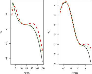
Figure 1: The estimates of the nonpararmetric components: $\widehat{\eta}_{1}$ and $\widehat{\eta}_{2}$. The solid, dotted and dashed curves correspond to the estimates under WI, AR(1) and RSM structures.

7 Discussion

We have developed a general methodology for simultaneously selecting variables and estimating the unknown components in APLMs for longitudinal and clustered data. We propose a one-step least squares approach to obtain the estimation of both the parametric and nonparametric components based on polynomial spline smoothing. This approach is flexible, computationally simple and very easy to implement in practice. We demonstrate that the asymptotic normality of the estimated coefficients for the linear part is retained. The proposed penalized regression method also achieves an “oracle” property in the sense that it performs as well as if the subset of significant parametric components were known in advance.

In this paper, our primary interest is the linear components, and we treat the nonparametric functions as nuisance components; thus we limit our discussions to estimation and variable selection for the linear part. Nonetheless, this may be extended to the nonparametric components using techniques similar to those in Xue [37]. An anonymous referee pointed out the feasibility of obtaining the asymptotic “oracle” property of the nonparametric components in Ma and Yang [24]. We believe that this property can be similarly obtained via a two-step spline backfitted kernel smoothing procedure (Ma and Yang [24]). However, the technical details deserve careful consideration, and this is an interesting topic of future research.

The simulation result indicates that the variable selection is consistent even if the correlation structure is misspecified. However, misspecification may lead to some efficiency loss. So, it would be desirable if one could choose an appropriate correlation structure based on available data in practice. The simulation results clearly show that there is marked improvement of efficiency when one uses the correct correlation structure though the variable selection seems to be consistent with misspecified structure. To select the correlation matrix, one might consider some resampling-based methods, such as the bootstrap and cross-validation methods in Pan and Connett [28] and other techniques in Diggle et al. [5]. There is, however, a clear need to formalize the procedures with solid theoretical justification. Instead of modeling the correlation through the “working” correlation matrix, one could also nonparametrically model the variance–covariance as some unknown smooth function (Chiou and Müller [4]). This is an excellent research problem for future study.

Appendix

For any vector $\mathbf{x}=(x_{1},\ldots,x_{d})^{\mathrm{T}}$, we denote $\|\cdot\|$ the usual Euclidean norm, that is, $\|\mathbf{x}\|=\sqrt{\sum_{k=1}^{d}x_{k}^{2}}$, and $\|\cdot\|_{\infty}$ the sup norm, that is, $\|\mathbf{x}\|_{\infty}=\sup_{1\leq k\leq d}|x_{k}|$. For any functions $\phi,\varphi$, let $\phi(\underline{\mathbf{X}}_{i},\underline{\mathbf{Z}}_{i})$ and $\varphi(\underline{\mathbf{X}}_{i},\underline{\mathbf{Z}}_{i})$ be $m_{i}$-vectors; then define the empirical inner product and the empirical norm as $\langle\phi,\varphi\rangle_{n}\equiv\langle\phi,\varphi\rangle_{n,\mathbf{V}}=n^{-1}\sum_{i=1}^{n}\phi(\underline{\mathbf{X}}_{i},\underline{\mathbf{Z}}_{i})^{\mathrm{T}}\mathbf{V}_{i}^{-1}\varphi(\underline{\mathbf{X}}_{i},\underline{\mathbf{Z}}_{i})$, $\|\phi\|_{n}^{2}=\langle\phi,\phi\rangle_{n}$, for the working covariance $\mathbf{V}_{i}$. Further denote $E_{n}(\phi)=\break n^{-1}\sum_{i=1}^{n}\mathbf{1}_{m_{i}}^{\mathrm{T}}\mathbf{V}_{i}^{-1}\phi(\underline{\mathbf{X}}_{i},\underline{\mathbf{Z}}_{i})$. If functions $\phi,\varphi$ are $L^{2}$-integrable, we define the theoretical inner product and its corresponding theoretical $L^{2}$ norm as $\langle\phi,\varphi\rangle=E(\langle\phi,\varphi\rangle_{n})$, $\|\phi\|^{2}=E(\|\phi\|_{n}^{2})$. Let $\widehat{\Pi}_{n}$ and $\Pi_{n}$ denote, respectively, the projection onto $G_{n}^{0}$ relative to the empirical and theoretical inner products. For convenience, let $h=h_{n}\sim J_{n}^{-1}$ and $\mathbf{I}_{d}$ be the $d\times d$ identity matrix.

.1 Proof of Theorem 1

Lemma A.1

Define

$$A_{n} = \sup_{g_{1},g_{2}\in G_{n}^{0}}|\langle g_{1},g_{2}\rangle_{n}-\langle g_{1},g_{2}\rangle|\|g_{1}\|^{-1}\|g_{2}\|^{-1},$$

$$B_{n} = \max_{1\leq k\leq d_{1}}\sup_{g\in G_{n}^{0}}\bigl{|}\|x_{k}-g\|_{n}^{2}/\|x_{k}-g\|^{2}-1\bigr{|},$$

then $A_{n}=\mathrm{O}_{P}\{\sqrt{\log(n)/(nh^{2})}\}$ and $B_{n}=\mathrm{O}_{P}\{\sqrt{\log(n)/(nh^{2})}\}$.

Lemma A.1 can be proved similarly to Lemmas A2 and A3 in Huang, Zhang and Zhou [14] and are thus omitted.

To obtain the closed-form expression of $\widehat{\bolds{\beta}}$, we need the following block form of the inverse of $\sum_{i=1}^{n}\underline{\mathbf{D}}_{i}^{\mathrm{T}}\mathbf{V}_{i}^{-1}\underline{\mathbf{D}}_{i}$:

$$\pmatrix{\displaystyle\sum_{i=1}^{n}\underline{\mathbf{X}}_{i}^{\mathrm{T}}\mathbf{V}_{i}^{-1}\underline{\mathbf{X}}_{i}&\displaystyle\sum_{i=1}^{n}\underline{\mathbf{X}}_{i}^{\mathrm{T}}\mathbf{V}_{i}^{-1}\underline{\mathbf{B}}_{i}\vspace*{2pt}\cr\displaystyle\sum_{i=1}^{n}\underline{\mathbf{B}}_{i}^{\mathrm{T}}\mathbf{V}_{i}^{-1}\underline{\mathbf{X}}_{i}&\displaystyle\sum_{i=1}^{n}\underline{\mathbf{B}}_{i}^{\mathrm{T}}\mathbf{V}_{i}^{-1}\underline{\mathbf{B}}_{i}}^{-1}=\pmatrix{\mathbf{H}_{\mathbf{XX}}&\mathbf{H}_{\mathbf{XB}}\vspace*{2pt}\cr\mathbf{H}_{\mathbf{BX}}&\mathbf{H}_{\mathbf{BB}}}^{-1}=\pmatrix{\mathbf{H}^{11}&\mathbf{H}^{12}\vspace*{2pt}\cr\mathbf{H}^{21}&\mathbf{H}^{22}},$$ (A.1)

where $\mathbf{H}^{11}=(\mathbf{H}_{\mathbf{XX}}-\mathbf{H}_{\mathbf{XB}}\mathbf{H}_{\mathbf{BB}}^{-1}\mathbf{H}_{\mathbf{BX}})^{-1}$, $\mathbf{H}^{22}=(\mathbf{H}_{\mathbf{BB}}-\mathbf{H}_{\mathbf{BX}}\mathbf{H}_{\mathbf{XX}}^{-1}\mathbf{H}_{\mathbf{XB}})^{-1}$, $\mathbf{H}^{12}=-\mathbf{H}^{11}\mathbf{H}_{\mathbf{XB}}\mathbf{H}_{\mathbf{BB}}^{-1}$ and $\mathbf{H}^{21}=-\mathbf{H}^{22}\mathbf{H}_{\mathbf{BX}}\mathbf{H}_{\mathbf{XX}}^{-1}$. Consequently,

$$\widehat{\bolds{\beta}}=\mathbf{H}^{11}\Biggl{\{}\sum_{i=1}^{n}\underline{\mathbf{X}}_{i}^{\mathrm{T}}\mathbf{V}_{i}^{-1}\underline{\mathbf{Y}}_{i}-\mathbf{H}_{\mathbf{XB}}\mathbf{H}_{\mathbf{BB}}^{-1}\sum_{i=1}^{n}\underline{\mathbf{B}}_{i}^{\mathrm{T}}\mathbf{V}_{i}^{-1}\underline{\mathbf{Y}}_{i}\Biggr{\}}.$$ (A.2)

Lemma A.2

Under Assumptions (A1)–(A5), for $\mathbf{H}_{\mathbf{BB}}$ in (A.1), one has (i) there exist constants $0<c_{H}<C_{H}$, $C_{H}^{\ast}=c_{H}^{-1},c_{H}^{\ast}=C_{H}^{-1}$ such that

$$c_{H}\mathbf{I}_{d_{2}J_{n}}\leq E(n^{-1}\mathbf{H}_{\mathbf{BB}})\leq C_{H}\mathbf{I}_{d_{2}J_{n}};$$ (A.3)

(ii) with probability approaching $1$ as $n\rightarrow\infty$,

$$c_{H}\mathbf{I}_{d_{2}J_{n}}\leq n^{-1}\mathbf{H}_{\mathbf{BB}}\leq C_{H}\mathbf{I}_{d_{2}J_{n}}.$$ (A.4)

Since the proof of Lemma A.2 is a little complicated, we provide it in the supplemental article (Ma, Song and Wang [23]). The proofs of Lemmas A.3 to A.7 below are also provided in (Ma, Song and Wang [23]).

Lemma A.3

Define $\widehat{\mathbf{U}}=(\sum_{i=1}^{n}\underline{\mathbf{B}}_{i}^{\mathrm{T}}\underline{\mathbf{X}}_{i})_{d_{2}J_{n}\times d_{1}}$, where $\underline{\mathbf{B}}_{i}$ is given in (3). Under Assumptions (A1)–(A5), there exist constants $0<c_{U}<C_{U}<\infty$, such that with probability approaching $1$ as $n\rightarrow\infty$, $c_{U}\mathbf{I}_{d_{1}}\leq(n^{-1}h)\widehat{\mathbf{U}}^{\mathrm{T}}\widehat{\mathbf{U}}\leq C_{U}\mathbf{I}_{d_{1}}.$

Lemma A.4

Under Assumptions (A1)–(A5), there exist constants $0<c_{H_{1}}<C_{H_{1}}<\infty$, such that with probability approaching $1$ as $n\rightarrow\infty$, $c_{H_{1}}\mathbf{I}_{d_{1}}\leq n\mathbf{H}^{11}\leq C_{H_{1}}\mathbf{I}_{d_{1}}$, where $\mathbf{H}^{11}$ is given in (A.1).

Let $\widetilde{\bolds{\beta}}_{\mu}$ and $\widetilde{\bolds{\beta}}_{e}$ be the solutions of (A.2) with $\underline{\mathbf{Y}}_{i}$ replaced by $\underline{\bolds{\mu}}_{i}$ and $\underline{\mathbf{e}}_{i}=\underline{\mathbf{Y}}_{i}-\underline{\bolds{\mu}}_{i}$, respectively. Then $\widehat{\bolds{\beta}}-\bolds{\beta}_{0}=(\widetilde{\bolds{\beta}}_{\mu}-\bolds{\beta}_{0})+\widetilde{\bolds{\beta}}_{e}$.

Lemma A.5

Under Assumptions (A1)–(A5), $\|\widetilde{\bolds{\beta}}_{\mu}-\bolds{\beta}_{0}\|=\mathrm{o}_{P}(n^{-1/2})$.

Note that $\widetilde{\bolds{\beta}}_{e}=\mathbf{H}^{11}\{\sum_{i=1}^{n}\underline{\mathbf{X}}_{i}^{\mathrm{T}}\mathbf{V}_{i}^{-1}\mathbf{\underline{e}}_{i}-\mathbf{H}_{\mathbf{XB}}\mathbf{H}_{\mathbf{BB}}^{-1}\sum_{i=1}^{n}\underline{\mathbf{B}}_{i}^{\mathrm{T}}\mathbf{V}_{i}^{-1}\underline{\mathbf{e}}_{i}\}$; thus we can show that the conditional variance $\mathrm{\mathrm{Var}}(\widetilde{\bolds{\beta}}_{e}|\mathbb{X},\mathbb{Z})$ equals

$$\mathbf{H}^{11}\sum_{i=1}^{n}\{\underline{\mathbf{X}}_{i}-\underline{\mathbf{B}}_{i}\mathbf{H}_{\mathbf{BB}}^{-1}\mathbf{H}_{\mathbf{BX}}\}^{\mathrm{T}}\mathbf{V}_{i}^{-1}\bolds{\Sigma}_{i}\mathbf{V}_{i}^{-1}\{\underline{\mathbf{X}}_{i}-\underline{\mathbf{B}}_{i}\mathbf{H}_{\mathbf{BB}}^{-1}\mathbf{H}_{\mathbf{BX}}\}\mathbf{H}^{11}.$$ (A.5)

Lemma A.6

Under Assumptions (A1)–(A5), as $n\rightarrow\infty$,

$$\{\mathrm{Var}(\widetilde{\bolds{\beta}}_{e}|\mathbb{X},\mathbb{Z})\}^{-1/2}(\widetilde{\bolds{\beta}}_{e})\longrightarrow N(0,\mathbf{I}_{d_{1}}).$$

Lemma A.7

Under Assumptions (A1)–(A5), for the covariance matrix $\bolds{\Omega}(\mathbb{V},\mathbb{\mathbb{\Sigma}})$ defined in (15), $c_{V}^{\ast}\mathbf{I}_{d_{1}}\leq\bolds{\Omega}(\mathbb{V},\mathbb{\mathbb{\Sigma}})\bolds{\leq}C_{V}^{\ast}\mathbf{I}_{d_{1}}$ and $\mathrm{Var}(\widetilde{\bolds{\beta}}_{e}|\mathbb{X},\mathbb{Z})=n^{-1}\bolds{\Omega}(\mathbb{V},\mathbb{\mathbb{\Sigma}})+\mathrm{O}_{P}(n^{-3/2}+n^{-1}h^{2p})$.

Theorem 1 follows from Lemmas A.5, A.6 and A.7.

.2 Proof of Theorem 2

From (12) and (A.1), we obtain

$$\widehat{\bolds{\gamma}}=\mathbf{H}^{22}\Biggl{(}\sum_{i=1}^{n}\underline{\mathbf{B}}_{i}^{\mathrm{T}}\mathbf{V}_{i}^{-1}\underline{\mathbf{Y}}_{i}-\mathbf{H}_{\mathbf{BX}}\mathbf{H}_{\mathbf{XX}}^{-1}\sum_{i=1}^{n}\underline{\mathbf{X}}_{i}^{\mathrm{T}}\mathbf{V}_{i}^{-1}\underline{\mathbf{Y}}_{i}\Biggr{)}.$$ (A.6)

Following the same idea as that in the proof of Lemma A.4, we have that there exist constants $0<c_{H_{2}}<C_{H_{2}}<\infty$, such that with probability approaching $1$ as $n\rightarrow\infty$, $c_{H_{2}}\mathbf{I}_{d_{2}J_{n}}\leq n\mathbf{H}^{22}\leq C_{H_{2}}\mathbf{I}_{d_{2}J_{n}}$. Letting $\widetilde{\bolds{\gamma}}_{\mu}$ and $\widetilde{\bolds{\gamma}}_{e}$ be the solutions of (A.6) with $\underline{\mathbf{Y}}_{i}$ replaced by $\underline{\bolds{\mu}}_{i}$ and $\mathbf{\underline{{e}}}_{i}=\underline{\mathbf{Y}}_{i}-\underline{\bolds{\mu}}_{i}$, respectively, $\widehat{\bolds{\gamma}}-\bolds{\gamma}=(\widetilde{\bolds{\gamma}}_{\mu}-\bolds{\gamma})+\widetilde{\bolds{\gamma}}_{e}$. Letting $\widehat{\Pi}_{n,\mathbf{X}}$ be the projection on $\{\underline{\mathbf{X}}_{i}\}_{i=1}^{n}$ to the empirical inner product, $\widetilde{\bolds{\gamma}}_{\mu}-\bolds{\gamma}$ equals

$$\mathbf{H}^{22}\Biggl{[}\sum_{i=1}^{n}\underline{\mathbf{B}}_{i}^{\mathrm{T}}\mathbf{V}_{i}^{-1}\Biggl{\{}\sum_{l=1}^{d_{2}}\eta_{l}(\mathbf{Z}_{il})\Biggr{\}}-\mathbf{H}_{\mathbf{BX}}\mathbf{H}_{\mathbf{XX}}^{-1}\sum_{i=1}^{n}\underline{\mathbf{X}}_{i}^{\mathrm{T}}\mathbf{V}_{i}^{-1}\Biggl{\{}\sum_{l=1}^{d_{2}}\eta_{l}(\mathbf{Z}_{il})\Biggr{\}}\Biggr{]}-\bolds{\gamma}$$

$$\quad=\mathbf{H}^{22}\sum_{i=1}^{n}\underline{\mathbf{B}}_{i}^{\mathrm{T}}\mathbf{V}_{i}^{-1}\Biggl{[}\Biggl{\{}\sum_{l=1}^{d_{2}}\eta_{l}(\mathbf{Z}_{il})-\underline{\mathbf{B}}_{i}\bolds{\gamma}\Biggr{\}}-\widehat{\Pi}_{n,\mathbf{X}}\Biggl{\{}\sum_{l=1}^{d_{2}}\eta_{l}(\mathbf{Z}_{il})-\underline{\mathbf{B}}_{i}\bolds{\gamma}\Biggr{\}}\Biggr{]}$$

$$\quad=n\mathbf{H}^{22}\mathbf{S},$$

where $\mathbf{S}=(S_{11},\ldots,S_{J_{n}d_{2}})$, with

$$S_{s,l}=n^{-1}\sum_{i=1}^{n}\bigl{(}\mathbf{B}_{i}^{(s,l)}\bigr{)}^{\mathrm{T}}\mathbf{V}_{i}^{-1}\Biggl{[}\Biggl{\{}\sum_{l=1}^{d_{2}}\eta_{l}(\mathbf{Z}_{il})-\underline{\mathbf{B}}_{i}\bolds{\gamma}\Biggr{\}}-\widehat{\Pi}_{n,\mathbf{X}}\Biggl{\{}\sum_{l=1}^{d_{2}}\eta_{l}(\mathbf{Z}_{il})-\underline{\mathbf{B}}_{i}\bolds{\gamma}\Biggr{\}}\Biggr{]},$$

and $\mathbf{B}_{i}^{(s,l)}=[\{B_{s,l}(Z_{i1l}),\ldots,B_{s,l}(Z_{im_{i}l})\}^{\mathrm{T}}]_{m_{i}\times 1}$. Let $\Delta\eta(\underline{\mathbf{Z}}_{i})=$ $\sum_{l=1}^{d_{2}}\eta_{l}(\mathbf{Z}_{il})-\underline{\mathbf{B}}_{i}\bolds{\gamma}$, then the Cauchy–Schwarz inequality implies that

$$|S_{s,l}|\leq\Biggl{\{}n^{-1}\sum_{i=1}^{n}\bigl{(}\mathbf{B}_{i}^{(s,l)}\bigr{)}^{\mathrm{T}}\mathbf{V}_{i}^{-1}\mathbf{B}_{i}^{(s,l)}\Biggr{\}}^{1/2}\|\Delta\eta-\widehat{\Pi}_{n,\mathbf{X}}(\Delta\eta)\|_{n}=\mathrm{O}_{P}(h^{p}),$$

thus $\|\widetilde{\bolds{\gamma}}_{\mu}-\bolds{\gamma}\|=$ $\mathrm{O}_{P}(J_{n}^{1/2}h^{p})$. For any $\mathbf{c}\in\mathcal{R}^{J_{n}d_{2}}$ with $\|\mathbf{c}\|=1$, we write $\mathbf{c}^{\mathrm{T}}\widetilde{\bolds{\gamma}}_{e}=\sum_{i=1}^{n}a_{i}\varepsilon_{i}$,  where $\varepsilon_{i}$ are independent conditioning on $(\mathbb{X},\mathbb{Z})$ and

$$a_{i}^{2}=\mathbf{c}^{\mathrm{T}}\mathbf{H}^{22}\{\underline{\mathbf{B}}_{i}-\underline{\mathbf{X}}_{i}\mathbf{H}_{\mathbf{XX}}^{-1}\mathbf{H}_{\mathbf{XB}}\}^{\mathrm{T}}\mathbf{V}_{i}^{-1}\bolds{\Sigma}_{i}\mathbf{V}_{i}^{-1}\{\underline{\mathbf{B}}_{i}-\underline{\mathbf{X}}_{i}\mathbf{H}_{\mathbf{XX}}^{-1}\mathbf{H}_{\mathbf{XB}}\}\mathbf{H}^{22}\mathbf{c}.$$

Following the same arguments as those in Lemma A.6, we have $\max_{1\leq i\leq n}|a_{i}|=\mathrm{O}_{P}(J_{n}^{1/2}n^{-1})$. Thus $\|\widetilde{\bolds{\gamma}}_{e}\|\leq J_{n}^{1/2}|\mathbf{c}^{\mathrm{T}}\widetilde{\bolds{\gamma}}_{e}|=J_{n}^{1/2}|\sum_{i=1}^{n}a_{i}\varepsilon_{i}|=\mathrm{O}_{P}(J_{n}^{1/2}n^{-1/2})$. Therefore, $\|\widehat{\bolds{\gamma}}_{l}-\bolds{\gamma}_{l}\|=\mathrm{O}_{P}(J_{n}^{1/2}h^{p}+J_{n}^{1/2}n^{-1/2})$. Because $\widehat{\eta}_{l}(z_{l})=\mathbf{B}_{l}^{\ast}(z_{l})^{\mathrm{T}}\widehat{\bolds{\gamma}}_{l}$, $\widetilde{\eta}_{l}(z_{l})=\mathbf{B}_{l}^{\ast}(z_{l})^{\mathrm{T}}\bolds{\gamma}_{l}$ and $|\widehat{\eta}_{l}-\widetilde{\eta}_{l}|_{L_{2}}^{2}=\|\widehat{\bolds{\gamma}}_{l}-\bolds{\gamma}_{l}\|^{2}\times\mathrm{O}_{P}(1)=\mathrm{O}_{P}(J_{n}h^{2p}+J_{n}n^{-1})$. Thus one has

$$|\widehat{\eta}_{l}-\eta_{l}|_{L_{2}}^{2}\leq 2(|\widehat{\eta}_{l}-\widetilde{\eta}_{l}|_{L_{2}}^{2}+|\widetilde{\eta}_{l}-\eta_{l}|_{L_{2}}^{2})=\mathrm{O}_{P}(J_{n}h^{2p}+J_{n}n^{-1}).$$

.3 Proof of Theorem 3

Let $\tau_{n}=n^{-1/2}+a_{n}$. It suffices to show that for any given $\zeta>0$, there exists a large constant $C$ such that

$$P\Bigl{\{}\sup_{\|\mathbf{u}\|=C}Q_{\mathcal{P}}(\bolds{\beta}_{0}+\tau_{n}\mathbf{u})>Q_{\mathcal{P}}(\bolds{\beta}_{0})\Bigr{\}}\geq 1-\zeta.$$ (A.7)

Plugging $\bolds{\gamma}(\bolds{\beta})$ in (7) into $Q(\bolds{\beta})$ defined in (2), we have

$$Q(\bolds{\beta}) = \frac{1}{2}\sum_{i=1}^{n}\Biggl{[}\mathbf{Y}_{i}-\Biggl{\{}\underline{\mathbf{X}}_{i}\bolds{\beta}+\underline{\mathbf{B}}_{i}\mathbf{H}_{\mathbf{BB}}^{-1}\sum_{i=1}^{n}\mathbf{B}_{i}^{\mathrm{T}}\mathbf{V}_{i}^{-1}(\mathbf{Y}_{i}-\underline{\mathbf{X}}_{i}\bolds{\beta})\Biggr{\}}\Biggr{]}^{\mathrm{T}}$$

$$\phantom{\frac{1}{2}\sum_{i=1}^{n}}{}\times\mathbf{V}_{i}^{-1}\Biggl{[}\mathbf{Y}_{i}-\Biggl{\{}\underline{\mathbf{X}}_{i}\bolds{\beta}+\underline{\mathbf{B}}_{i}\mathbf{H}_{\mathbf{BB}}^{-1}\sum_{i=1}^{n}\underline{\mathbf{B}}_{i}^{\mathrm{T}}\mathbf{V}_{i}^{-1}(\mathbf{Y}_{i}-\underline{\mathbf{X}}_{i}\bolds{\beta})\Biggr{\}}\Biggr{]}.$$

Thus $Q(\bolds{\beta})=\frac{1}{2}\sum_{i=1}^{n}(\mathbf{Y}_{i}-\widehat{\underline{\mathbf{X}}}_{i}\bolds{\beta}-\widehat{\Pi}_{n}\mathbf{Y}_{i})^{\mathrm{T}}\mathbf{V}_{i}^{-1}(\mathbf{Y}_{i}-\widehat{\underline{\mathbf{X}}}_{i}\bolds{\beta}-\widehat{\Pi}_{n}\mathbf{Y}_{i}).$ Let $U_{n,1}=Q(\bolds{\beta}_{0}+\tau_{n}\mathbf{u})-Q(\bolds{\beta}_{0})$ and $U_{n,2}=n_{\mathrm{T}}\sum_{k=1}^{r}\{p_{\lambda_{k}}(|\beta_{k0}+\tau_{n}u_{k}|)-p_{\lambda_{k}}(|\beta_{k0}|)\}$, where $r$ is the number of components of $\bolds{\beta}_{10}$. Note that $p_{\lambda_{k}}(0)=0$ and $p_{\lambda_{k}}(|\beta|)\geq 0$ for all $\beta$. Thus, $Q_{\mathcal{P}}(\bolds{\beta}_{0}+\tau_{n}\mathbf{u})-Q_{\mathcal{P}}(\bolds{\beta}_{0})\geq U_{n,1}+U_{n,2}$.

For $U_{n,1}$, we have $Q(\bolds{\beta}_{0}+\tau_{n}\mathbf{u})=Q(\bolds{\beta}_{0})+\tau_{n}\mathbf{u}^{\mathrm{T}}\dot{Q}(\bolds{\beta}_{0})+\frac{1}{2}\tau_{n}^{2}\mathbf{u}^{\mathrm{T}}\ddot{Q}(\bolds{\beta}^{\ast})\mathbf{u},$ where $\ddot{Q}(\bolds{\beta})=\sum_{i=1}^{n}\widehat{\underline{\mathbf{X}}}_{i}^{\mathrm{T}}\mathbf{V}_{i}^{-1}\widehat{\underline{\mathbf{X}}}_{i}$, $\bolds{\beta}^{\ast}=t(\bolds{\beta}_{0}+n^{-1/2}\mathbf{u})+(1-t)\bolds{\beta}_{0}$, $t\in[0,1]$. Note that

$$\dot{Q}(\bolds{\beta}_{0}) = \sum_{i=1}^{n}\widehat{\underline{\mathbf{X}}}_{i}^{\mathrm{T}}\mathbf{V}_{i}^{-1}(\mathbf{Y}_{i}-\widehat{\underline{\mathbf{X}}}_{i}\bolds{\beta}_{0}\mathbf{-}\widehat{\Pi}_{n}\mathbf{Y}_{i})$$

$$= \sum_{i=1}^{n}\widehat{\underline{\mathbf{X}}}_{i}^{\mathrm{T}}\mathbf{V}_{i}^{-1}\Biggl{\{}\sum_{l=1}^{d_{2}}\eta_{l}(\mathbf{Z}_{il})-\widehat{\Pi}_{n}\sum_{l=1}^{d_{2}}\eta_{l}(\mathbf{Z}_{il})\Biggr{\}}+\sum_{i=1}^{n}\widehat{\underline{\mathbf{X}}}_{i}^{\mathrm{T}}\mathbf{V}_{i}^{-1}(\underline{\mathbf{e}}_{i}-\widehat{\Pi}_{n}\underline{\mathbf{e}}_{i}),$$

where $\underline{\mathbf{e}}_{i}=\underline{\mathbf{Y}}_{i}-\underline{\bolds{\mu}}_{i}$. Mimicking the proof for Lemmas A.5 and A.6, we have

$$\sum_{i=1}^{n}\widehat{\underline{\mathbf{X}}}_{i}^{\mathrm{T}}\mathbf{V}_{i}^{-1}\Biggl{\{}\sum_{l=1}^{d_{2}}\eta_{l}(\mathbf{Z}_{il})-\widehat{\Pi}_{n}\sum_{l=1}^{d_{2}}\eta_{l}(\mathbf{Z}_{il})\Biggr{\}} = \mathrm{o}_{P}(n^{1/2}),$$

$$\sum_{i=1}^{n}\widehat{\underline{\mathbf{X}}}_{i}^{\mathrm{T}}\mathbf{V}_{i}^{-1}(\underline{\mathbf{e}}_{i}-\widehat{\Pi}_{n}\underline{\mathbf{e}}_{i}) = \mathrm{O}_{P}(n^{1/2}).$$

Thus $\tau_{n}\mathbf{u}^{\mathrm{T}}\dot{Q}(\bolds{\beta}_{0})=\mathrm{O}_{P}(n^{1/2}\tau_{n})\|\mathbf{u}\|$. By the proof of Lemma A.4, we obtain that $\frac{1}{2}\tau_{n}^{2}\mathbf{u}^{\mathrm{T}}\times\ddot{Q}(\bolds{\beta}_{0})\mathbf{u}=\mathrm{O}_{P}(n\tau_{n}^{2})+\mathrm{o}_{P}(1)$. Thus

$$U_{n,1}=\mathrm{O}_{P}(n^{1/2}\tau_{n})+\mathrm{O}_{P}(n\tau_{n}^{2})+\mathrm{o}_{P}(1).$$ (A.8)

For $U_{n,2}$, by a Taylor expansion,

$$p_{\lambda_{k}}(|\beta_{k0}+\tau_{n}u_{k}|)=p_{\lambda_{k}}(|\beta_{k0}|)+\tau_{n}u_{k}p_{\lambda_{k}}^{\prime}(|\beta_{k0}|)\mathrm{sgn}(\beta_{k0})+{\textstyle\frac{1}{2}}\tau_{n}^{2}u_{k}^{2}p_{\lambda_{k}}^{\prime\prime}(|\beta_{k}^{\ast}|),$$

where $\beta_{k}^{\ast}=(1-t)\beta_{k0}+t(\beta_{k0}+n^{-1/2}u_{k})$, $t\in[0,1]$ and

$$p_{\lambda_{k}}(|\beta_{k0}+\tau_{n}u_{k}|)=p_{\lambda_{k}}(|\beta_{k0}|)+\tau_{n}u_{k}p_{\lambda_{k}}^{\prime}(|\beta_{k0}|)\mathrm{sgn}(\beta_{k0})+{\textstyle\frac{1}{2}}\tau_{n}^{2}u_{k}^{2}p_{\lambda_{k}}^{\prime\prime}(|\beta_{k0}|)+\mathrm{o}(n^{-1}).$$

Thus, by the Cauchy–Schwarz inequality,

$$n_{\mathrm{T}}^{-1}U_{n,2} = \tau_{n}\sum_{k=1}^{r}u_{k}p_{\lambda_{k}}^{\prime}(|\beta_{k0}|)\mathrm{sgn}(\beta_{k0})+\frac{1}{2}\tau_{n}^{2}\sum_{k=1}^{r}u_{k}^{2}p_{\lambda_{k}}^{\prime\prime}(|\beta_{k0}|)$$

$$\leq \sqrt{r}\tau_{n}a_{n}\|\mathbf{u}\|+\frac{1}{2}\tau_{n}^{2}w_{n}\|\mathbf{u}\|^{2}=C\tau_{n}^{2}\bigl{(}\sqrt{r}+w_{n}C\bigr{)}.$$

As $w_{n}\rightarrow 0$, the first two terms on the right-hand side of (A.8) dominate $U_{n,2}$ by taking $C$ sufficiently large. Hence (A.7) holds for sufficiently large $C$.

.4 Proof of Theorem 4

We first show that the estimator $\widehat{\bolds{\beta}}^{\mathrm{P}}$ must possess the sparsity property $\widehat{\bolds{\beta}}_{2}=0$, which is stated as follows.

Lemma A.8

Under the conditions of Theorem 4, with probability tending to 1, for any given $\bolds{\beta}_{1}$ satisfying that $\|\bolds{\beta}_{1}-\bolds{\beta}_{10}\|=\mathrm{O}_{P}(n^{-1/2})$ and any constant $C$,

$$Q_{\mathcal{P}}\{(\bolds{\beta}_{1}^{\mathrm{T}},\mathbf{0}^{\mathrm{T}})^{\mathrm{T}}\}=\min_{\|\bolds{\beta}_{2}\|\leq Cn^{-1/2}}Q_{\mathcal{P}}\{(\bolds{\beta}_{1}^{\mathrm{T}},\bolds{\beta}_{2}^{\mathrm{T}})\}.$$

Proof.

To prove that the maximizer is obtained at $\bolds{\beta}_{2}=0$, it suffices to show that with probability tending to 1, as $n\rightarrow\infty$, for any $\bolds{\beta}_{1}$ satisfying $\|\bolds{\beta}_{1}-\bolds{\beta}_{10}\|=\mathrm{O}_{P}(n^{-1/2})$, and $\|\bolds{\beta}_{2}\|\leq Cn^{-1/2}$, $\partial Q_{\mathcal{P}}(\bolds{\beta})/\partial\beta_{k}$ and $\beta_{k}$ have different signs for $\beta_{k}\in(-Cn^{-1/2},Cn^{-1/2})$, for $k=r+1,\ldots,d_{1}$. Note that

$$\dot{Q}_{\mathcal{P},k}(\bolds{\beta})\equiv\frac{\partial Q_{\mathcal{P}}(\bolds{\beta})}{\partial\beta_{k}}=\dot{Q}_{k}(\bolds{\beta})+n_{\mathrm{T}}p_{\lambda_{kn}}^{\prime}(|\beta_{k}|)\operatorname{sgn}(\beta_{k}),$$

where $\dot{Q}_{k}(\bolds{\beta})=\dot{Q}_{k}(\bolds{\beta}_{0})+\sum_{k^{\prime}=1}^{d_{1}}\ddot{Q}_{kk^{\prime}}\{t\beta_{k^{\prime}}+(1-t)\beta_{0k^{\prime}}\}(\beta_{k^{\prime}}-\beta_{0k^{\prime}})$, $t\in[0,1]$,

$$\dot{Q}_{k}(\bolds{\beta}_{0})=e_{k}^{\mathrm{T}}\sum_{i=1}^{n}\widehat{\underline{\mathbf{X}}}_{i}^{\mathrm{T}}\mathbf{V}_{i}^{-1}(\mathbf{Y}_{i}-\widehat{\underline{\mathbf{X}}}_{i}\bolds{\beta}_{0}-\widehat{\Pi}_{n}\mathbf{Y}_{i}).$$

It follows by the similar arguments as given in the proofs of Theorems 1 and 3 that

$$\dot{Q}_{k}(\bolds{\beta}_{0}) = e_{k}^{\mathrm{T}}\sum_{i=1}^{n}\widehat{\underline{\mathbf{X}}}_{i}^{\mathrm{T}}\mathbf{V}_{i}^{-1}\Biggl{\{}\sum_{l=1}^{d_{2}}\eta_{l}(\mathbf{Z}_{il})-\widehat{\Pi}_{n}\sum_{l=1}^{d_{2}}\eta_{l}(\mathbf{Z}_{il})\Biggr{\}}+e_{k}^{\mathrm{T}}\sum_{i=1}^{n}\widehat{\underline{\mathbf{X}}}_{i}^{\mathrm{T}}\mathbf{V}_{i}^{-1}(\underline{\mathbf{e}}_{i}-\widehat{\Pi}_{n}\underline{\mathbf{e}}_{i})$$

$$= n\Biggl{\{}n^{-1}\sum_{i=1}^{n}\Xi_{k}(\underline{\mathbf{Y}}_{i},\underline{\mathbf{X}}_{i},\bolds{\underline{Z}}_{i})+\mathrm{o}_{P}(n^{-1/2})\Biggr{\}},$$

where $\Xi_{k}(\underline{\mathbf{Y}}_{i},\underline{\mathbf{X}}_{i},\underline{\mathbf{Z}}_{i})$ is the $k$th element of matrix $\widehat{\underline{\mathbf{X}}}_{i}^{\mathrm{T}}\mathbf{V}_{i}^{-1}(\underline{\mathbf{e}}_{i}-\widehat{\Pi}_{n}\underline{\mathbf{e}}_{i})$. According to Lemma A.7, we have

$$n^{-1}\ddot{Q}(\bolds{\beta}_{0}) = E\Biggl{(}n^{-1}\sum_{i=1}^{n}\widetilde{\underline{\mathbf{X}}}_{i}^{\mathrm{T}}\mathbf{V}_{i}^{-1}\widetilde{\underline{\mathbf{X}}}_{i}\Biggr{)}+\mathrm{o}_{P}(1)=\mathbf{R}+\mathrm{o}_{P}(1),$$

$$\frac{1}{n}\sum_{k^{\prime}=1}^{d_{1}}\ddot{Q}_{kk^{\prime}}(\beta_{k^{\prime}}-\beta_{0k^{\prime}}) = (\bolds{\beta}-\bolds{\beta}_{0})^{\mathrm{T}}\bigl{(}R_{k}+\mathrm{o}_{P}(1)\bigr{)},$$

where $R_{k}$ is the $k$th column of $\mathbf{R}$. Note that $\|\bolds{\beta}-\bolds{\beta}_{0}\|=\mathrm{O}_{P}(n^{-1/2})$ by the assumption. Thus, $n^{-1}\dot{Q}_{k}(\bolds{\beta})$ is of the order $\mathrm{O}_{P}(n^{-1/2})$. Therefore, for any nonzero $\beta_{k}$ and $k=r+1,\ldots,d_{1}$,

$$\dot{Q}_{\mathcal{P},k}(\bolds{\beta})=n\lambda_{kn}\biggl{\{}\lambda_{kn}^{-1}p_{\lambda_{kn}}^{\prime}(|\beta_{k}|)\operatorname{sgn}(\beta_{k})+\mathrm{O}_{P}\biggl{(}\frac{1}{\sqrt{n}\lambda_{kn}}\biggr{)}\biggr{\}}.$$

Since $\liminf_{n\rightarrow\infty}\liminf_{\beta_{k}\rightarrow 0^{+}}\lambda_{kn}^{-1}p_{\lambda_{kn}}^{\prime}(|\beta_{k}|)>0$ and $\sqrt{n}\lambda_{kn}\rightarrow\infty$, the sign of the derivative is determined by that of $\beta_{k}$. Thus the desired result is obtained. ∎

Proof of Theorem 4 From Lemma A.8, it follows that $\widehat{\bolds{\beta}}_{2}^{\mathrm{P}}=\mathbf{0}$.

$$\dot{Q}_{\mathcal{P}}(\bolds{\beta}) = \dot{Q}(\bolds{\beta}_{0})+\ddot{Q}(\bolds{\beta}^{\ast})(\bolds{\beta}-\bolds{\beta}_{0})+n_{\mathrm{T}}\{p_{\lambda_{kn}}^{\prime}(|\beta_{k0}|)\operatorname{sign}(\beta_{k0})\}_{k=1}^{r}$$

$${}+\Biggl{\{}\sum_{k=1}^{r}p_{\lambda_{kn}}^{\prime\prime}(|\beta_{k0}|)+\mathrm{o}_{P}(1)\Biggr{\}}(\widehat{\bolds{\beta}}\,_{k1}^{\mathrm{P}}-\beta_{k0}),$$

where $\bolds{\beta}^{\ast}=t\bolds{\beta}_{0}+(1-t)\bolds{\beta}$, $t\in[0,1]$. Using an argument similar to the proof of Theorem 3, it can be shown that there exists a $\widehat{\bolds{\beta}}_{1}^{\mathrm{P}}$ in Theorem 3 that is a root-$n$ consistent local minimizer of $Q_{\mathcal{P}}\{(\bolds{\beta}_{1}^{\mathrm{T}},\mathbf{0}^{{}^{\mathrm{T}}})^{\mathrm{T}}\}$, satisfying the penalized least squares equations $\dot{Q}_{\mathcal{P}}[\{(\widehat{\bolds{\beta}}_{1}^{\mathrm{P}})^{\mathrm{T}},\mathbf{0}^{{}^{\mathrm{T}}}\}^{\mathrm{T}}]=\mathbf{0}$. Mimicking the proofs for Lemmas A.5 and A.6 indicates that the left hand side of the above equation can be written as

$$n^{-1}\sum_{i=1}^{n}\widehat{\underline{\mathbf{X}}}_{1i}^{\mathrm{T}}\mathbf{V}_{i}^{-1}(\underline{\mathbf{e}}_{i}-\hat{\Pi}_{n}\underline{\mathbf{e}}_{i})+\{p_{\lambda_{kn}}^{\prime}(|\beta_{k0}|)\operatorname{sign}(\beta_{k0})\}_{k=1}^{r}+\mathrm{o}_{P}(n^{-1/2})$$

$$\quad{}+\Biggl{\{}E\Biggl{(}n^{-1}\sum_{i=1}^{n}\widetilde{\underline{\mathbf{X}}}_{1i}^{\mathrm{T}}\mathbf{V}_{i}^{-1}\widetilde{\underline{\mathbf{X}}}_{1i}\Biggr{)}+\mathrm{o}_{P}(1)\Biggr{\}}(\widehat{\bolds{\beta}}_{1}^{\mathrm{P}}-\bolds{\beta}_{10})$$

$$\quad{}+\Biggl{\{}\sum_{k=1}^{r}p_{\lambda_{kn}}^{\prime\prime}(|\beta_{k0}|)+\mathrm{o}_{P}(1)\Biggr{\}}(\widehat{\bolds{\beta}}_{1}^{\mathrm{P}}-\bolds{\beta}_{10}).$$

Thus we have

$$\mathbf{0} = n^{-1}\sum_{i=1}^{n}\widehat{\bolds{\underline{X}}}_{1i}^{\mathrm{T}}\mathbf{V}_{i}^{-1}(\underline{\mathbf{e}}_{i}-\hat{\Pi}_{n}\underline{\mathbf{e}}_{i})+\kappa_{n}+\mathrm{o}_{P}(n^{-1/2})$$

$${}+\Biggl{\{}E\Biggl{(}n^{-1}\sum_{i=1}^{n}\widetilde{\underline{\mathbf{X}}}_{1i}^{\mathrm{T}}\mathbf{V}_{i}^{-1}\widetilde{\underline{\mathbf{X}}}_{1i}\Biggr{)}+\bolds{\Sigma}_{\lambda}+\mathrm{o}_{P}(1)\Biggr{\}}(\widehat{\bolds{\beta}}_{1}^{\mathrm{P}}-\bolds{\beta}_{10}).$$

Similar arguments to Lemmas A.6 and A.7 yield the asymptotic normality.

References

• [1] {bmisc}[auto:STB—2011/11/23—09:42:52] \bauthor\bsnmAntoniadis, \bfnmA.\binitsA. (\byear1997). \bhowpublishedWavelets in statistics: A review (with discussion). Italian Jour. Statist. 6, 97–144. \bptokimsref \endbibitem
• [2] {barticle}[mr] \bauthor\bsnmCai, \bfnmJianwen\binitsJ., \bauthor\bsnmFan, \bfnmJianqing\binitsJ., \bauthor\bsnmLi, \bfnmRunze\binitsR. &\bauthor\bsnmZhou, \bfnmHaibo\binitsH. (\byear2005). \btitleVariable selection for multivariate failure time data. \bjournalBiometrika \bvolume92 \bpages303–316. \biddoi=10.1093/biomet/92.2.303, issn=0006-3444, mr=2201361 \bptokimsref \endbibitem
• [3] {barticle}[mr] \bauthor\bsnmCarroll, \bfnmRaymond J.\binitsR.J., \bauthor\bsnmMaity, \bfnmArnab\binitsA., \bauthor\bsnmMammen, \bfnmEnno\binitsE. &\bauthor\bsnmYu, \bfnmKyusang\binitsK. (\byear2009). \btitleNonparametric additive regression for repeatedly measured data. \bjournalBiometrika \bvolume96 \bpages383–398. \biddoi=10.1093/biomet/asp015, issn=0006-3444, mr=2507150 \bptokimsref \endbibitem
• [4] {barticle}[mr] \bauthor\bsnmChiou, \bfnmJeng-Min\binitsJ.M. &\bauthor\bsnmMüller, \bfnmHans-Georg\binitsH.G. (\byear2005). \btitleEstimated estimating equations: Semiparametric inference for clustered and longitudinal data. \bjournalJ. R. Stat. Soc. Ser. B Stat. Methodol. \bvolume67 \bpages531–553. \biddoi=10.1111/j.1467-9868.2005.00514.x, issn=1369-7412, mr=2168203 \bptokimsref \endbibitem
• [5] {bbook}[mr] \bauthor\bsnmDiggle, \bfnmPeter J.\binitsP.J., \bauthor\bsnmHeagerty, \bfnmPatrick J.\binitsP.J., \bauthor\bsnmLiang, \bfnmKung-Yee\binitsK.Y. &\bauthor\bsnmZeger, \bfnmScott L.\binitsS.L. (\byear2002). \btitleAnalysis of Longitudinal Data, \bedition2nd ed. \bseriesOxford Statistical Science Series \bvolume25. \baddressOxford: \bpublisherOxford Univ. Press. \bidmr=2049007 \bptokimsref \endbibitem
• [6] {barticle}[auto:STB—2011/11/23—09:42:52] \bauthor\bsnmFan, \bfnmJ.\binitsJ., \bauthor\bsnmFeng, \bfnmY.\binitsY. &\bauthor\bsnmSong, \bfnmR.\binitsR. (\byear2010). \btitleNonparametric independence screening in sparse ultra-high dimensional additive models. \bjournalJ. Amer. Statist. Assoc. \bvolume106 \bpages544–557. \bptokimsref \endbibitem
• [7] {barticle}[mr] \bauthor\bsnmFan, \bfnmJianqing\binitsJ. &\bauthor\bsnmLi, \bfnmRunze\binitsR. (\byear2001). \btitleVariable selection via nonconcave penalized likelihood and its oracle properties. \bjournalJ. Amer. Statist. Assoc. \bvolume96 \bpages1348–1360. \biddoi=10.1198/016214501753382273, issn=0162-1459, mr=1946581 \bptokimsref \endbibitem
• [8] {barticle}[mr] \bauthor\bsnmFan, \bfnmJianqing\binitsJ. &\bauthor\bsnmLi, \bfnmRunze\binitsR. (\byear2002). \btitleVariable selection for Cox’s proportional hazards model and frailty model. \bjournalAnn. Statist. \bvolume30 \bpages74–99. \biddoi=10.1214/aos/1015362185, issn=0090-5364, mr=1892656 \bptokimsref \endbibitem
• [9] {barticle}[mr] \bauthor\bsnmFan, \bfnmYanqin\binitsY. &\bauthor\bsnmLi, \bfnmQi\binitsQ. (\byear2003). \btitleA kernel-based method for estimating additive partially linear models. \bjournalStatist. Sinica \bvolume13 \bpages739–762. \bidissn=1017-0405, mr=1997172 \bptokimsref \endbibitem
• [10] {barticle}[mr] \bauthor\bsnmFu, \bfnmWenjiang J.\binitsW.J. (\byear2003). \btitlePenalized estimating equations. \bjournalBiometrics \bvolume59 \bpages126–132. \biddoi=10.1111/1541-0420.00015, issn=0006-341X, mr=1978479 \bptokimsref \endbibitem
• [11] {barticle}[mr] \bauthor\bsnmHall, \bfnmPeter\binitsP., \bauthor\bsnmMüller, \bfnmHans-Georg\binitsH.G. &\bauthor\bsnmWang, \bfnmJane-Ling\binitsJ.L. (\byear2006). \btitleProperties of principal component methods for functional and longitudinal data analysis. \bjournalAnn. Statist. \bvolume34 \bpages1493–1517. \biddoi=10.1214/009053606000000272, issn=0090-5364, mr=2278365 \bptokimsref \endbibitem
• [12] {bbook}[mr] \bauthor\bsnmHärdle, \bfnmWolfgang\binitsW., \bauthor\bsnmLiang, \bfnmHua\binitsH. &\bauthor\bsnmGao, \bfnmJiti\binitsJ. (\byear2000). \btitlePartially Linear Models: Contributions to Statistics. \baddressHeidelberg: \bpublisherPhysica-Verlag. \bidmr=1787637 \bptokimsref \endbibitem
• [13] {barticle}[mr] \bauthor\bsnmHuang, \bfnmJianhua Z.\binitsJ.Z., \bauthor\bsnmWu, \bfnmColin O.\binitsC.O. &\bauthor\bsnmZhou, \bfnmLan\binitsL. (\byear2004). \btitlePolynomial spline estimation and inference for varying coefficient models with longitudinal data. \bjournalStatist. Sinica \bvolume14 \bpages763–788. \bidissn=1017-0405, mr=2087972 \bptokimsref \endbibitem
• [14] {barticle}[mr] \bauthor\bsnmHuang, \bfnmJianhua Z.\binitsJ.Z., \bauthor\bsnmZhang, \bfnmLiangyue\binitsL. &\bauthor\bsnmZhou, \bfnmLan\binitsL. (\byear2007). \btitleEfficient estimation in marginal partially linear models for longitudinal/clustered data using splines. \bjournalScand. J. Statist. \bvolume34 \bpages451–477. \biddoi=10.1111/j.1467-9469.2006.00550.x, issn=0303-6898, mr=2368793 \bptnotecheck year \bptokimsref \endbibitem
• [15] {barticle}[mr] \bauthor\bsnmLi, \bfnmQi\binitsQ. (\byear2000). \btitleEfficient estimation of additive partially linear models. \bjournalInternat. Econom. Rev. \bvolume41 \bpages1073–1092. \biddoi=10.1111/1468-2354.00096, issn=0020-6598, mr=1790072 \bptokimsref \endbibitem
• [16] {barticle}[mr] \bauthor\bsnmLi, \bfnmRunze\binitsR. &\bauthor\bsnmLiang, \bfnmHua\binitsH. (\byear2008). \btitleVariable selection in semiparametric regression modeling. \bjournalAnn. Statist. \bvolume36 \bpages261–286. \biddoi=10.1214/009053607000000604, issn=0090-5364, mr=2387971 \bptokimsref \endbibitem
• [17] {barticle}[mr] \bauthor\bsnmLiang, \bfnmHua\binitsH. &\bauthor\bsnmLi, \bfnmRunze\binitsR. (\byear2009). \btitleVariable selection for partially linear models with measurement errors. \bjournalJ. Amer. Statist. Assoc. \bvolume104 \bpages234–248. \biddoi=10.1198/jasa.2009.0127, issn=0162-1459, mr=2504375 \bptokimsref \endbibitem
• [18] {barticle}[mr] \bauthor\bsnmLiang, \bfnmHua\binitsH., \bauthor\bsnmThurston, \bfnmSally W.\binitsS.W., \bauthor\bsnmRuppert, \bfnmDavid\binitsD., \bauthor\bsnmApanasovich, \bfnmTatiyana\binitsT. &\bauthor\bsnmHauser, \bfnmRuss\binitsR. (\byear2008). \btitleAdditive partial linear models with measurement errors. \bjournalBiometrika \bvolume95 \bpages667–678. \biddoi=10.1093/biomet/asn024, issn=0006-3444, mr=2443182 \bptokimsref \endbibitem
• [19] {barticle}[mr] \bauthor\bsnmLiang, \bfnmKung Yee\binitsK.Y. &\bauthor\bsnmZeger, \bfnmScott L.\binitsS.L. (\byear1986). \btitleLongitudinal data analysis using generalized linear models. \bjournalBiometrika \bvolume73 \bpages13–22. \biddoi=10.1093/biomet/73.1.13, issn=0006-3444, mr=0836430 \bptokimsref \endbibitem
• [20] {barticle}[mr] \bauthor\bsnmLin, \bfnmXihong\binitsX. &\bauthor\bsnmCarroll, \bfnmRaymond J.\binitsR.J. (\byear2001). \btitleSemiparametric regression for clustered data. \bjournalBiometrika \bvolume88 \bpages1179–1185. \biddoi=10.1093/biomet/88.4.1179, issn=0006-3444, mr=1872228 \bptokimsref \endbibitem
• [21] {barticle}[auto:STB—2011/11/23—09:42:52] \bauthor\bsnmLiu, \bfnmX.\binitsX., \bauthor\bsnmWang, \bfnmL.\binitsL. &\bauthor\bsnmLiang, \bfnmH.\binitsH. (\byear2011). \btitleEstimation and variable selection for semiparametric additive partial linear models. \bjournalStatist. Sinica. \bvolume21 \bpages1225–1248. \bptokimsref \endbibitem
• [22] {barticle}[mr] \bauthor\bsnmLiu, \bfnmYufeng\binitsY. &\bauthor\bsnmWu, \bfnmYichao\binitsY. (\byear2007). \btitleVariable selection via a combination of the $L_{0}$ and $L_{1}$ penalties. \bjournalJ. Comput. Graph. Statist. \bvolume16 \bpages782–798. \biddoi=10.1198/106186007X255676, issn=1061-8600, mr=2412482 \bptokimsref \endbibitem
• [23] {bmisc}[auto:STB—2011/11/23—09:42:52] \bauthor\bsnmMa, \bfnmS.\binitsS., \bauthor\bsnmSong, \bfnmQ.\binitsQ. &\bauthor\bsnmWang, \bfnmL.\binitsL. (\byear2011). \bhowpublishedSupplement to “Simultaneous variable selection and estimation in semiparametric modeling of longitudinal/clustered data”. DOI:10.3150/11-BEJ386SUPP. \bptokimsref \endbibitem
• [24] {barticle}[mr] \bauthor\bsnmMa, \bfnmShujie\binitsS. &\bauthor\bsnmYang, \bfnmLijian\binitsL. (\byear2011). \btitleSpline-backfitted kernel smoothing of partially linear additive model. \bjournalJ. Statist. Plann. Inference \bvolume141 \bpages204–219. \biddoi=10.1016/j.jspi.2010.05.028, issn=0378-3758, mr=2719488 \bptokimsref \endbibitem
• [25] {barticle}[mr] \bauthor\bsnmMa, \bfnmYanyuan\binitsY. &\bauthor\bsnmLi, \bfnmRunze\binitsR. (\byear2010). \btitleVariable selection in measurement error models. \bjournalBernoulli \bvolume16 \bpages274–300. \biddoi=10.3150/09-BEJ205, issn=1350-7265, mr=2648758 \bptokimsref \endbibitem
• [26] {barticle}[mr] \bauthor\bsnmMeinshausen, \bfnmNicolai\binitsN. &\bauthor\bsnmBühlmann, \bfnmPeter\binitsP. (\byear2006). \btitleHigh-dimensional graphs and variable selection with the lasso. \bjournalAnn. Statist. \bvolume34 \bpages1436–1462. \biddoi=10.1214/009053606000000281, issn=0090-5364, mr=2278363 \bptokimsref \endbibitem
• [27] {barticle}[auto:STB—2011/11/23—09:42:52] \bauthor\bsnmOpsomer, \bfnmJ. D.\binitsJ.D. &\bauthor\bsnmRuppert, \bfnmD.\binitsD. (\byear1999). \btitleA root-n consistent backfitting estimator for semiparametric additive modelling. \bjournalJ. Comput. Graph. Statist. \bvolume8 \bpages715–734. \bptokimsref \endbibitem
• [28] {barticle}[mr] \bauthor\bsnmPan, \bfnmWei\binitsW. &\bauthor\bsnmConnett, \bfnmJohn E.\binitsJ.E. (\byear2002). \btitleSelecting the working correlation structure in generalized estimating equations with application to the lung health study. \bjournalStatist. Sinica \bvolume12 \bpages475–490. \bidissn=1017-0405, mr=1902720 \bptokimsref \endbibitem
• [29] {barticle}[mr] \bauthor\bsnmStone, \bfnmCharles J.\binitsC.J. (\byear1985). \btitleAdditive regression and other nonparametric models. \bjournalAnn. Statist. \bvolume13 \bpages689–705. \biddoi=10.1214/aos/1176349548, issn=0090-5364, mr=0790566 \bptokimsref \endbibitem
• [30] {barticle}[mr] \bauthor\bsnmTibshirani, \bfnmRobert\binitsR. (\byear1996). \btitleRegression shrinkage and selection via the lasso. \bjournalJ. Roy. Statist. Soc. Ser. B \bvolume58 \bpages267–288. \bidissn=0035-9246, mr=1379242 \bptokimsref \endbibitem
• [31] {barticle}[pbm] \bauthor\bsnmTibshirani, \bfnmR.\binitsR. (\byear1997). \btitleThe lasso method for variable selection in the Cox model. \bjournalStat. Med. \bvolume16 \bpages385–395. \bidissn=0277-6715,pii=10.1002/(SICI)1097-0258(19970228)16:4¡385::AID-SIM380¿3.0.CO;2-3,pmid=9044528 \bptokimsref \endbibitem
• [32] {barticle}[mr] \bauthor\bsnmWang, \bfnmJane-Ling\binitsJ.L., \bauthor\bsnmXue, \bfnmLiugen\binitsL., \bauthor\bsnmZhu, \bfnmLixing\binitsL. &\bauthor\bsnmChong, \bfnmYun Sam\binitsY.S. (\byear2010). \btitleEstimation for a partial-linear single-index model. \bjournalAnn. Statist. \bvolume38 \bpages246–274. \biddoi=10.1214/09-AOS712, issn=0090-5364, mr=2589322 \bptokimsref \endbibitem
• [33] {barticle}[mr] \bauthor\bsnmWang, \bfnmLi\binitsL. &\bauthor\bsnmYang, \bfnmLijian\binitsL. (\byear2007). \btitleSpline-backfitted kernel smoothing of nonlinear additive autoregression model. \bjournalAnn. Statist. \bvolume35 \bpages2474–2503. \biddoi=10.1214/009053607000000488, issn=0090-5364, mr=2382655 \bptokimsref \endbibitem
• [34] {barticle}[mr] \bauthor\bsnmWang, \bfnmNaisyin\binitsN. (\byear2003). \btitleMarginal nonparametric kernel regression accounting for within-subject correlation. \bjournalBiometrika \bvolume90 \bpages43–52. \biddoi=10.1093/biomet/90.1.43, issn=0006-3444, mr=1966549 \bptokimsref \endbibitem
• [35] {barticle}[mr] \bauthor\bsnmWang, \bfnmNaisyin\binitsN., \bauthor\bsnmCarroll, \bfnmRaymond J.\binitsR.J. &\bauthor\bsnmLin, \bfnmXihong\binitsX. (\byear2005). \btitleEfficient semiparametric marginal estimation for longitudinal/clustered data. \bjournalJ. Amer. Statist. Assoc. \bvolume100 \bpages147–157. \biddoi=10.1198/016214504000000629, issn=0162-1459, mr=2156825 \bptokimsref \endbibitem
• [36] {barticle}[mr] \bauthor\bsnmWu, \bfnmYichao\binitsY. &\bauthor\bsnmLiu, \bfnmYufeng\binitsY. (\byear2009). \btitleVariable selection in quantile regression. \bjournalStatist. Sinica \bvolume19 \bpages801–817. \bidissn=1017-0405, mr=2514189 \bptokimsref \endbibitem
• [37] {barticle}[mr] \bauthor\bsnmXue, \bfnmLan\binitsL. (\byear2009). \btitleConsistent variable selection in additive models. \bjournalStatist. Sinica \bvolume19 \bpages1281–1296. \bidissn=1017-0405, mr=2536156 \bptokimsref \endbibitem
• [38] {barticle}[mr] \bauthor\bsnmXue, \bfnmLan\binitsL., \bauthor\bsnmQu, \bfnmAnnie\binitsA. &\bauthor\bsnmZhou, \bfnmJianhui\binitsJ. (\byear2010). \btitleConsistent model selection for marginal generalized additive model for correlated data. \bjournalJ. Amer. Statist. Assoc. \bvolume105 \bpages1518–1530. \biddoi=10.1198/jasa.2010.tm10128, issn=0162-1459, mr=2796568 \bptokimsref \endbibitem
• [39] {barticle}[mr] \bauthor\bsnmXue, \bfnmLan\binitsL. &\bauthor\bsnmYang, \bfnmLijian\binitsL. (\byear2006). \btitleAdditive coefficient modeling via polynomial spline. \bjournalStatist. Sinica \bvolume16 \bpages1423–1446. \bidissn=1017-0405, mr=2327498 \bptokimsref \endbibitem
• [40] {barticle}[mr] \bauthor\bsnmYang, \bfnmYuhong\binitsY. (\byear2008). \btitleLocalized model selection for regression. \bjournalEconometric Theory \bvolume24 \bpages472–492. \biddoi=10.1017/S0266466608080195, issn=0266-4666, mr=2391618 \bptokimsref \endbibitem
• [41] {barticle}[mr] \bauthor\bsnmYuan, \bfnmMing\binitsM. &\bauthor\bsnmLin, \bfnmYi\binitsY. (\byear2007). \btitleOn the non-negative garrote estimator. \bjournalJ. R. Stat. Soc. Ser. B Stat. Methodol. \bvolume69 \bpages143–161. \biddoi=10.1111/j.1467-9868.2007.00581.x, issn=1369-7412, mr=2325269 \bptokimsref \endbibitem
• [42] {barticle}[pbm] \bauthor\bsnmZeger, \bfnmS. L.\binitsS.L. &\bauthor\bsnmDiggle, \bfnmP. J.\binitsP.J. (\byear1994). \btitleSemiparametric models for longitudinal data with application to CD4 cell numbers in HIV seroconverters. \bjournalBiometrics \bvolume50 \bpages689–699. \bidissn=0006-341X, pmid=7981395 \bptokimsref \endbibitem