Comparing Polarised Synchrotron and Thermal Dust Emission in the Galactic Plane

Abstract

As the next step toward an improved large scale Galactic magnetic field model, we present a simple comparison of polarised synchrotron and thermal dust emission on the Galactic plane. We find that the field configuration in our previous model that reproduces the polarised synchrotron is not compatible with the WMAP 94 GHz polarised emission data. In particular, the high degree of dust polarisation in the outer Galaxy ($90\degr<\ell<270\degr$) implies that the fields in the dust-emitting regions are more ordered than the average of synchrotron-emitting regions. This new dust information allows us to constrain the spatial mixing of the coherent and random magnetic field components in the outer Galaxy. The inner Galaxy differs in polarisation degree and apparently requires a more complicated scenario than our current model. In the scenario that each interstellar component (including fields and now dust) follows a spiral arm modulation, as observed in external galaxies, the changing degree of ordering of the fields in dust-emitting regions may imply that the dust arms and the field component arms are shifted as a varying function of Galacto-centric radius. We discuss the implications for how the spiral arm compression affects the various components of the magnetised interstellar medium but conclude that improved data such as that expected from the Planck satellite will be required for a thorough analysis.

1 Introduction

Determining the large-scale structure of the Galactic magnetic fields is a longstanding and difficult task. The fields are important to a variety of astrophysical phenomena from star formation to cosmic ray propagation, but there are few ways of observing them directly. Radio astronomy is the primary way that we study magnetic fields, but any analysis in only one domain is subject to a variety of degeneracies that cannot be disentangled without several complementary measurements and a multi-wavelength approach.

Jaffe et al. (2010); Jaffe et al. (2011) model the large-scale Galactic magnetic fields in the plane using a combination of three observables: the total and polarised intensity of diffuse synchrotron emission, and Faraday rotation measures (RMs) of extra-galactic sources. Other analyses of the large-scale magnetic fields have been performed using the full sky (e.g., Sun et al. 2008, Fauvet et al. 2011; Fauvet et al. 2012, Jansson et al. 2009; Jansson & Farrar 2012) or the high-latitude sky (Strong et al., 2011). We focus on the plane in order to probe through the full Galactic disk in detail, and we now continue these studies with the addition of the polarised thermal dust emission. In addition to being an independent tracer of the field direction, the dust emission follows a different spatial distribution and therefore is not subject to the same uncertainties as previous studies using only synchrotron emission.

An important aspect of our previous work is to separate the fields into components defined by their observational signatures. As described in Jaffe et al. (2010), the coherent fields contribute to both polarised emission as well as to RM, while isotropic random fields contribute only to the total intensity of the diffuse emission. A third component is needed to include the effect of anisotropy in the turbulence, a component that maintains a common ordered axis but changes direction stochastically. This “ordered random” field component contributes to polarised emission but not to RM.

Since the cosmic ray electron (CRE) distribution is thought to be fairly smooth (see § 4 for a discussion), the contributions to the synchrotron emission from the different magnetic field components do not depend strongly on their relative spatial locations. Our aim is therefore to add the information from the polarised dust emission from WMAP to study the spatial distribution of each component. The geometry of how the polarised emission relates to the different magnetic field components is identical for diffuse thermal dust emission. But the distribution of dust is not as smooth as the CRE distribution and is known to peak in spiral arms (see, e.g., Drimmel & Spergel 2001). This allows us to probe whether the field components peak in the same ridges or whether, as seen in external galaxies (Beck, 2009), different components may lie along different arms that may have different pitch angles or be shifted relative to each other. Note that WMAP W-band at 94 GHz primarily probes the relatively cold dust, which has a different spatial distribution from the hotter dust dominating the infra-red.

We hope also to shed light on the outstanding question of arm versus inter-arm contrasts in the components of the magnetised interstellar medium (ISM). In external galaxies, Fletcher et al. (2011) and references therein do not find the contrast in synchrotron emission between arms and inter-arm regions as predicted by the scenario of compression in the spiral arm shocks. It remains unclear if this is due to the limited resolution of the current observations in external galaxies. Our method comparing the complementary observables of synchrotron, dust, and RMs along with a variety of external constraints allows us to ask similar questions from within the plane of the Milky Way.

We test a model of the magnetised ISM where each component contains a spiral arm structure but the arm peaks are not necessarily spatially coincident. In particular, we address the question of how to reproduce the level of dust polarisation in the outer Galaxy (defined as $90\degr<\ell<270\degr$, i.e. quadrants two and three). This region is dominated by the Perseus arm that passes outward of the Sun’s position. The outer Galaxy is therefore ideal to model unambiguously the arms of the different components, since we are looking through one inter-arm region and one arm ridge, beyond which is expected to be very little ISM. The inner Galaxy (defined as $-90\degr<\ell<90\degr$, i.e. quadrants one and four) is more complicated, and there are already indications that the large-scale field structure is not a simple spiral (van Eck et al. 2011).

Our simple comparison of polarised synchrotron and dust emission in the outer Galaxy allows us to study the relative positions of the arms as well as the arm versus inter-arm contrasts. This is analogous to studies such as Patrikeev et al. (2006) or Fletcher et al. (2011) perform on M51 but with a very different perspective from within the disk. This is important to understand the relationship between the magnetic fields and other components of the ISM and the effect of spiral arm compression on all components. We can test the scenario where gas, dust, and fields are compressed in the spiral arm shock, which predicts strongly ordered fields in the dust-emitting regions. We further discuss the implications of these results for the inner Galaxy and outline future work.

We describe the data we use in § 2 and the modelling and simulation methods in § 3. We then discuss the inputs and existing constraints on the various components of the magnetised ISM in § 4. We show the results of our simulations in § 5 and discuss the implications in § 6, along with outlining the further work these results point toward.

2 Data

Following our previous work, we use a combination of low-frequency radio as well as microwave data, in total and polarised intensity, and examine the profiles in longitude of each frequency along the Galactic plane.

2.1 Radio and low-frequency microwave datasets

The datasets and references are summarised in Table 1. We use the 408 MHz survey by Haslam et al. (1982), the WMAP 23 GHz polarisation map from Jarosik et al. (2011), and three catalogues of RMs, the Southern and Canadian Galactic Plane Surveys (SGPS and CGPS) of Brown et al. (2003); Brown et al. (2007) and the additional catalogue from van Eck et al. (2011).

Each of the emission maps in HEALPix (Górski et al., 2005) format is smoothed to a common low resolution of FWHM $6\degr$ and downgraded to $N_{\mathrm{side}}=32$. The RM catalogues are averaged into bins at the same resolution and assigned error bars based on the RMS variation of the individual measures within the bin. The profiles in longitude along the plane are shown in Fig. 1 along with a comparison to an updated form of our previous model (Jaffe et al., 2011) as described in § 3.1. (Note that we do not attempt to fit the region within 10$\degr$ of the Galactic centre, and the model is not plotted there.)

In order to use the low-frequency radio observations in total intensity on the plane, we apply a correction to remove most of the free-free emission. As described in Jaffe et al. (2011), we find that the WMAP MEM free-free solution at 33 GHz appears to overestimate the thermal contribution. We found, using simple cross-correlations, that a normalization factor of 0.8 appears to give a good correction to the radio frequencies, and we use it in the dust band total intensity at 94 GHz as well. In both cases, the template is extrapolated to each corrected frequency with the spectrum given in Dickinson et al. (2003). This component has been subtracted from the total intensity profiles in green in Fig. 1 and is also shown in orange for comparison.

Note that the polarised intensity, $PI=\sqrt{Q^{2}+U^{2}}$ plotted in Fig. 1 is subject to a noise bias due to the squaring of the noise on $Q$ and $U$. In the case of the synchrotron polarisation on the plane, the polarisation bias is too small to see. But for the dust polarisation at 94 GHz, this bias is significant. To reduce it, we combine the data from different WMAP years into two independent maps each of $Q$ and $U$, and then construct $\mathrm{x}PI=\sqrt{Q_{1}Q_{2}+U_{1}U_{2}}$. Since the noise contributions in $Q_{1}$ and $Q_{2}$ are independent, this cross estimator of the polarised intensity has little noise bias and roughly equivalent uncertainties. A better estimator of $PI$ would depend on the detailed properties of the detectors, and for the quantitative analyses in our previous work we used $Q$ and $U$ separately, but for the qualitative analysis presented here, this $\mathrm{x}PI$ is quite informative.

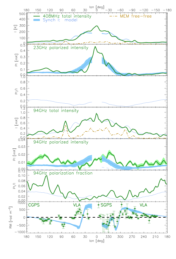
Figure 1: Profiles of the observables (thick green lines) and the slightly updated version of our previously fitted model (thin blue lines) along the Galactic plane. See text in § 2. In order from the top: total intensity at 408 MHz minus free-free estimate; polarised intensity at 23 GHz; model synchrotron polarisation fraction; total intensity at 94 GHz minus free-free estimate; polarised intensity at 94 GHz and (as the pale green filled region) its uncertainty (see text in § 2.2); dust polarisation fraction; Faraday RM at 1.4 GHz. The shaded regions show the Galactic variance for the model, i.e. the expected variation due to the turbulence. The dashed line in the dust panels shows the modelled synchrotron contribution at 94 GHz, which is small but not negligible. The dot-dashed gold line shows the free-free estimate compared to the total intensity curves.

Survey	Frequency [GHz]	Original resolution	Coverage	Reference
Haslam	0.408	$\sim$51 arcmin	Full sky	Haslam et al. (1982)
WMAP 7-year	22.8	53 arcmin	Full Sky	Jarosik et al. (2011)
WMAP 7-year	94	13 arcmin	Full Sky	Jarosik et al. (2011)
CGPS RMs	1.4	1 arcmin	part of Northern plane; see Fig. 1	Brown et al. (2003)
SGPS RMs	1.4	100 arcsec	part of Southern plane; see Fig. 1	Brown et al. (2007)
VLA RMs	1.4	50 arcsec	part of plane; see Fig. 1	van Eck et al. (2011)

Table 1: The datasets used in this analysis. The RMs are the extra-galactic sources only from the Canadian Galactic Plane survey (CGPS), the Southern Galactic Plane Survey (SGPS) and the van Eck et al. survey using the Very Large Array (VLA).

2.2 WMAP 94 GHz polarisation

The new dataset we include in this work is the WMAP 94 GHz frequency that, in polarisation, is dominated by thermal dust emission. As can be seen in Fig. 1, the free-free emission correction is also necessary on the plane, but unlike at 23 GHz, it does not dominate the total intensity.

The calibration and signal-to-noise ratio of the 94 GHz polarisation is more of a concern, however, since the dust emission is more weakly polarised than synchrotron emission. As noted above, the noise bias is significant at 94 GHz, which we overcome by plotting $\mathrm{x}PI$. We can also characterise the noise and calibration uncertainties by comparison of the maps for individual years. We use the variance from year to year in $Q$ and $U$ to estimate the uncertainty on $\mathrm{x}PI$, which then includes the effects of both the noise and the systematic uncertainties that are of that time-scale. These uncertainties are plotted as the dotted green lines around the green $\mathrm{x}PI$profile in Fig. 1. Jarosik et al. (2011) single out the W4 difference assembly as particularly prone to systematic artefacts, and we find that including it does significantly increase our estimate of the uncertainties. We therefore follow Jarosik et al. and omit W4 from the analysis.

The S/N apparent in Fig. 1 is somewhat low for performing quantitative fits and parameter exploration but is sufficient for the simpler qualitative analysis we present here. For a thorough exploration of the parameter space, we will need better data such as that expected from the Planck mission (Planck Collaboration, 2011).

3 Methods

The methods and tools used in this work are described in Jaffe et al. (2010), Jaffe et al. (2011), and Fauvet et al. (2011). In short, we have adopted models for each of the physical components of the ISM (thermal electrons, magnetic fields, dust, and CREs) and then integrated through the Galactic plane to simulate observable polarised emission and Faraday RM for comparison to the data.

As discussed in § 2.2, the WMAP 94 GHz polarisation data do not have a high enough S/N for a quantitative analysis such as the MCMC parameter exploration. So for this work, we simply compare the profiles and draw qualitative conclusions from the morphology.

3.1 Models of the Galaxy components

We use a magnetic field model based on a spiral arm compression as described in Jaffe et al. (2010). We have improved this model somewhat to simplify the parametrization and to make the field continuous and closer to divergence-free. See Appendix A for the modified parametrization. The principle differences are: to remove the extra complexity of the radial profile in the innermost few kpc of the Galaxy that originally followed Broadbent (1989) but is excluded in this analysis; to define the transition between arms continuously (rather than to jump discontinuously in the inter-arm region as in the previous parametrization); to vary the width of each arm with Galacto-centric radius in inverse proportion to the coherent field strength. Remember that the coherent field is assumed parallel to the arm, so that the arm corresponds to a magnetic flux tube. This last modification, which conserves magnetic flux, maintains a roughly divergence-free field. We also allow the spiral arm patterns for the different components (which are otherwise similar) to vary independently in orientation about the Galactic north-south pole. In other words, the components’ arms can be shifted relative to each other by a constant angle.

As in Jaffe et al. (2011), we use the “NE2001” thermal electron distribution model of Cordes & Lazio (2002).

We also use the galprop cosmic ray propagation code with a model based on the “z04LMPDS” from Strong et al. (2010) and with the fitted injection spectrum from Jaffe et al. (2011). Based on the given distribution of CRE sources, the code determines the spatial and spectral distribution of CREs after propagation in the Galaxy’s magnetic fields, in this case our model rather than the galprop model. The resulting distribution then is taken to compute the synchrotron emission as described in § 3.2.

We use a dust distribution model based on the same spiral arm parametrization used for the magnetic fields, which is in fact similar to that of Drimmel & Spergel (2001). Our parameters, given in Table 3, are adjusted to match the integrated total intensity profile of the data at 94 GHz. Fig. 1 shows that the model profile matches well at large scales.

We use the dust polarisation model described in Fauvet et al. (2011), i.e. with a geometrical factor of $\sin(\alpha)^{3}$, where $\alpha$ is the angle between the local field orientation and the line-of-sight (LOS). This factor approximates the effects of grain alignment and projection onto the LOS, but we note that our analysis is not particularly sensitive to this factor.

3.2 Simulation of observables

As described in Jaffe et al. (2010), we simulate the diffuse polarised emission at large scales using the publicly available code hammurabi (Waelkens et al., 2009), which simulates observables such as synchrotron and dust emission in full Stokes parameters and Faraday RMs. Jaffe et al. (2011) described how we then linked this code to the Galprop cosmic ray propagation code in order to include high-energy constraints from both direct cosmic-ray measurements or from diffuse $\gamma$-ray emission as measured by the Fermi LAT (Ackermann et al., 2010; Abdo et al., 2009). This is important to compare the synchrotron total intensity at low radio frequencies with polarised intensity at microwave frequencies. (Since low frequency polarisation is affected by Faraday depolarisation and higher frequencies by free-free contamination on the plane, it is complicated to compare total and polarised intensities on the plane at the same frequency.) Parameters have simply been adjusted manually to match the data as plotted in profiles along the plane as in Fig. 1. (A quantitative parameter exploration will be performed in a future work.)

Fauvet et al. use hammurabi to compute the “geometric suppression” map, i.e. the map of the polarisation fraction, and multiply it by a total intensity template to scale the polarisation simulation. This allows a more accurate modelling, since the intensity template partly accounts for localised features not in the model. In Fig. 2, we follow the same approach, using the 94 GHz total intensity data corrected for the free-free emission as described in Jaffe et al. (2011). This is in contrast to Fig. 1, where we do not use a template but simply plot the result of the integration through our dust density model. In this case, both the data and the simulated total intensity profiles are plotted for comparison, and their very similar large-scale characteristics give confidence that the dust distribution model should be accurate enough for this analysis.

As described in Waelkens et al. (2009), the simulation resolution in hammurabi is refined with radius as the observed solid angle encompasses a larger volume. The result is a resolution that varies but does not increase significantly with radius. In our large-scale, low-resolution simulations, it is roughly 20 pc or larger. With an outer scale of turbulence of 100 pc, this is clearly not sensitive to more than the largest scales of the turbulence (represented by a Gaussian random field simulation). Any structure on scales smaller than this will be modeled only as an average over the “sub-grid” effects. We have tested that increasing the resolution does not impact our results. The maps themselves are simulated to match observations smoothed to 6$\degr$ as described in § 2 above.

4 Inputs and Constraints

We use our previously studied models and additional information from other studies that is relevant to the comparison of data and model. In the following, we explain the choices we have made and the relevant external constraints.

4.1 Synchrotron

In Jaffe et al. (2010); Jaffe et al. (2011), we constrained the ratios of the magnetic field components (defined above) using synchrotron total and polarised emission as well as Faraday rotation measure. For the current analysis, we retain largely the same model as in Jaffe et al. (2011) but allow for an azimuthal shift between the spiral patterns of the different components. This has little effect on the integrated synchrotron profiles, since the model CRE distribution is relatively smooth and varies slowly with Galacto-centric radius.

4.2 Arm versus inter-arm contrast

The theory of shock compression at a spiral arm predicts a gas density contrast of approximately a factor of 4 in the shocked versus the pre-shock medium, assuming a strong adiabatic shock (e.g., Landau & Lifshitz 1987). The components of the magnetic field that are parallel to the shock are therefore compressed as well and thus amplified by a factor of 4. This is the physical motivation for the creation of the ordered random field from the isotropic random field and for the amplification of the coherent field, which is parallel to the same spiral shock front in our model.

We do not model the shock itself but simple spiral arms with Gaussian profiles. This can be thought of as a large-scale approximation to the modulation of a shock that then re-expands to its pre-shock strength downstream. We can define a contrast as the ratio of the peak in the arm to the minimum between arms. The original model of Broadbent et al. (1990) used a contrast of 3.5 for both coherent and isotropic random field components, which they found reproduced well the synchrotron total intensity profile, particularly the amplitude of the emission observed in the direction of spiral arm tangents.

We use the Broadbent et al. value of 3.5 as a starting value, but in our model, the strength of the coherent field component in each arm is allowed to vary as in Jaffe et al. (2010) so as to be consistent with the RM data. This contrast then varies for each arm by the factor $a_{i}$ given in Table 2. But these values cannot be compared with the theoretical value of 4 for shocked versus pre-shock medium without some knowledge of the width of the shocked region and its re-expansion, since our Gaussian profiles are effectively a large-scale average. Note also that the coherent field strengths in the arms we choose to match the RM data are degenerate with the thermal electron distribution, which is not very precisely known.

The ordered random component increases at the shock as a result of compression of both any pre-shock ordered random field and of the pre-shock isotropic random field. It then decreases back to its pre-shock strength, due to both re-expansion across the spiral arm and re-isotropisation by supernova-driven turbulence after star formation triggered by the shock. There are also other possible sources of the ordered random component such as superbubbles or shearing motions. In our model, this component has a Gaussian profile that goes to zero between the arms (and therefore has no meaningful contrast), so this is clearly only a simple approximation to include a variety of physical effects.

The isotropic random component itself would remain unchanged through the shock, only providing the source of an ordered random field created there. Our modeled spiral arm modulation of the isotropic random component therefore has a different origin such as the supernova-driven turbulence downstream of the shock. The arm contrast is therefore not constrained a priori and is left at the Broadbent et al. value of 3.5.

The diffuse component of the gas and dust would also be compressed by a factor of 4 in the shock, but the average gas and dust density is more strongly compressed due to the formation of dense clouds behind the shock. Since the WMAP data at 94 GHz trace primarily the cold dust component, it in particular will be tracing a more strongly compressed average density. For our dust model, we use the same parametrized spiral arm modulation but with a contrast of 7. This value, however, is degenerate with other parameters such as the dust arm width.

Our adopted contrasts are therefore either unconstrained a priori or roughly compatible with the loose theoretical constraint from the shock scenario. We will show that we can reproduce the degree of polarisation in the data in the outer Galaxy with our current choices, but we note that this will not provide a unique solution. Additional data on the distribution of both the dust and the fields in the Galaxy will be needed to create an unambiguous model of the effects of compression on the ISM in the spiral arms.

4.3 Cosmic ray arm contrast

The situation for CREs is somewhat different from that of the magnetic fields and dust. Similarly to the thermal gas, CREs can be considered to be tied to field lines, so that they should undergo the same perpendicular compression as the field. However, in the realistic situation where the shock front is not infinite and/or the field has a small component across the shock, CREs would diffuse along field lines at roughly the Alfvén speed, thereby reducing their post-shock density. An additional effect, clearly discussed in Fletcher et al. (2011), is that the perpendicular momentum squared of each CRE should increase at the shock in direct proportion to the field strength – by virtue of the conservation of the first adiabatic invariant (e.g., Northrop 1963). This would lead to an overall shift of the CRE energy spectrum towards higher energies, and hence to an additional increase (typically by the same factor of 4 as for the gas and the magnetic field) in the number density of CREs with a given energy, e.g. the characteristic energy for a given radio synchrotron observation.

From these two different effects on the CREs, each of which may lead to a factor of 4 compression, the number density of CREs at a given energy is expected to increase at the spiral-arm shock by a factor between 4 and 16. This abrupt increase in density would then be smoothed out on the downstream side, on roughly a diffusion length, $L\sim\sqrt{Dt}$, where $D$ is the diffusion coefficient (usually assumed to be isotropic for simplicity) and $t$ is the CRE lifetime. With $D\sim 3\times 10^{28}~{}{\rm cm^{2}~{}s^{-1}}$ and $t\sim(10^{7}-10^{8})$ yrs for electrons of a few GeV in a field of a few $\upmu$G, the diffusion length works out to be $L\sim(1-3)$ kpc.

Another aspect that might affect our analysis is the question of anisotropic diffusion of CRs from their acceleration sites. Effenberger et al. (2012), for example, simulate the propagation of CR protons including anisotropic diffusion in the presence of a spiral magnetic field. They find that if the CR sources are also distributed along spiral arms, the resulting CR density retains a strong azimuthal modulation, with an amplitude ratio as large as a factor of $\simeq 6$ for strongly anisotropic diffusion (as opposed to only $\simeq 2$ for isotropic diffusion) in the case of 1 GeV protons. Note that this effect is completely separate from, and not necessarily spatially coincident with, the CRE modulation due to the spiral-arm shock itself.

The question of whether the CRE distribution varies from arm to inter-arm regions is therefore a relevant uncertainty in our analysis.

Ackermann et al. (2011) present a study of the third Galactic quadrant where comparison of the $\gamma$-ray data with the velocity cubes in HI allows a separation of the spiral arms from the inter-arm regions. Among their results is a measure of the $\gamma$-ray emissivity in each region. They find that the $\gamma$-ray emission properties, when normalised by the varying gas density, vary little as a function of Galacto-centric radius. The small ($\approx 5$ per cent) average difference between the arm and inter-arm region implies a slightly lower emissivity per unit gas density in the Perseus arm compared to the inter-arm region that lies just inward of it. Though this is an analysis based on CR nucleon interactions rather than CR electrons, there is as yet no evidence in favour of any CR enhancement in the Perseus arm.

Since no enhancement as large as predicted has so far been observed either toward our Galaxy’s Perseus arm or in M51 (Fletcher et al., 2011), we consider our model of a smooth, azimuthally symmetric CRE distribution to be sufficiently realistic for this first-order analysis. We discuss the small effect a CRE enhancement in the arm might have on our results in § 5.

4.4 Dust intrinsic polarisation fraction

The details of the thermal dust emission process, and in particular the alignment of the grains with the magnetic field, are not well understood (Draine & Fraisse, 2009). There are therefore few theoretical constraints on the intrinsic polarisation fraction of dust, in contrast to the case of synchrotron, which introduces an additional uncertainty into the analysis. Observations of nearby, high-latitude clouds, which are likely observed at nearly their intrinsic polarisation, have dust polarisation fractions of up to $\sim$20 per cent with most much lower (Benoît et al., 2004; Ponthieu et al., 2005; Fauvet et al., 2011).

As we will discuss further below, the interesting differences between our model and the observations include the overall level of dust polarisation. We will show that we can address this problem in the outer Galaxy by changing the spatial distribution of the magnetic field components relative to each other and to the dust emitting regions. In other words, a higher than expected polarisation fraction can be reproduced by increasing either the intrinsic polarisation or the degree of ordering in the fields in the dust emitting regions; the two questions are degenerate. Adopting a higher degree of intrinsic polarisation is therefore the conservative choice that avoids over-stating the data’s ability to constrain the field ordering.

As described in § 3.2, our simulation has a finite resolution that in this large-scale study is of order 20 pc. The number we use as the “intrinsic” polarisation fraction is therefore the assumed average degree of polarization from a region of this size. Since the average molecular cloud size is of the same scale, this fraction then represents an average over a cloud. We might improve the modeling of the sub-grid effects, i.e. include the turbulence driven within the clouds with a model that could be significantly different in both scale and amplitude from what we have modeled for synchrotron. This improvement, however, could only decrease the predicted degree of polarisation from that obtained assuming an intrinsic polarisation of 30 per cent.

We therefore adopt 30 per cent for the intrinsic polarization fraction as a conservative upper limit while noting that this value is degenerate with the question of how ordered the fields are in the dust emitting regions.

4.5 External galaxies

External galaxies have been mapped in both total and polarised intensity by low-frequency radio observations. Beck (2009) reviews the different morphologies seen and in particular, the different relationships observed between the spiral structure seen in polarised synchrotron emission and that seen in gas tracers. A study of M51 by Fletcher et al. (2011) provides one of the first estimates of arm versus inter-arm contrasts seen in polarised synchrotron emission. They find a much lower level of contrast than expected by the scenario of shock compression by the spiral wave, but they note that it is unclear whether their observations have sufficient resolution. Their limit on the size of the compressed region based on the observed low level of contrast and the telescope beam is not so small as to rule out the scenario.

Patrikeev et al. (2006) use a wavelet analysis to find the arm ridges in each of a set of maps from low-frequency radio polarisation to CO and infra-red observations. They find a systematic shift in the molecular gas versus the mid-infrared in each spiral arm, consistent with the delay of star formation triggered in the shock. The polarised emission is also the component the furthest upstream, as expected if the magnetic fields are compressed and aligned with the shock.

Though these observations do not provide strong constraints on the relative positions or widths of the arms or on the arm versus inter-arm contrasts, they do provide evidence for such shifts and for variations between components’ arm geometries. As such, observations of external galaxies motivate our attempt to explore these differences in our own Galaxy.

5 Results

5.1 Profiles along the Galactic plane

Following Jaffe et al. (2010), we examine profiles of the observables along the Galactic plane as shown in Fig. 1. The model in blue is simply an updated form of our previous model from Jaffe et al. (2011). The RMs constrain the coherent field intensity in each arm, while the total and polarised synchrotron intensities constrain the amounts of isotropic and ordered random components.

We have added the dust emission as described in § 3.1 and see that the model (blue curve in Fig. 1) does not fit the dust polarised emission data at all, with two main problems. Firstly, the shape of the profile is not correct, with proportionately too much polarised emission in the inner Galaxy compared to the outer Galaxy. Secondly, in the outer Galaxy, the polarisation fraction is too low.

It is apparent from the RM panel of Fig. 1 that the data from van Eck et al. (2011) do not match our model. The geometry of our model was originally constrained in Jaffe et al. (2010) before these data were available. It is clear that though the amplitude of the closest peak in our RM model roughly matches the van Eck et al. data, its longitude does not. We note that simply changing the orientations of the spiral arms, their pitch angles (currently $-11.5\degr$), or the radius of the inner Galaxy ring does not solve the problem. Something more complicated than simple logarithmic spirals and an annular ring will be needed, but the average RM and its large scale variations predicted by our model are sufficiently accurate to fix the strength of the coherent field component.

It must also be noted that there is significant uncertainty regarding the distance to the Perseus arm in the outer Galaxy. The spiral arm model used in the NE2001 model places it roughly 2-3 kpc away toward the anti-centre, while the analysis of velocity data presented in both Abdo et al. (2010) and Ackermann et al. (2011) imply nearly twice the distance. There is a large degree of uncertainty in both estimates, but our analysis is not significantly affected by this. Our results are dependent only on the relative positions of the different components, not their absolute distances, and can therefore be re-scaled to match a corrected distance determination.

5.2 Outer Galaxy

For these simulations, we have assumed an intrinsic polarisation fraction of the dust of 30 per cent. As discussed in Section 4.4, 30 per cent is at the high end of what is considered plausible and significantly higher than what is usually assumed. By using 30 per cent, we are therefore being conservative, since a more commonly assumed 15 per cent makes the discrepancy between the model and the data in the outer Galaxy more extreme. An even higher intrinsic polarisation fraction might solve the problem in the outer Galaxy but would be in even more serious conflict with observations.

Nor can we reproduce the observed polarisation fraction by increasing the average amount of magnetic field ordering, because this would break the fit to the synchrotron emission. But since the synchrotron emission depends on the spatial distribution of CREs, and since these CREs quickly diffuse away from their acceleration sites (see discussion in Section 4.3), the synchrotron polarisation degree reflects only the average level of coherent and ordered random fields versus isotropic random fields. It is not very sensitive to where those components are spatially located. Therefore, we can shift the components relative to one another without much changing the synchrotron emission profiles.

We show the effect of this with a new model in yellow in Fig.  2, which is identical to the previous model except for the location of the isotropic random component. In the blue curve, as before, all field components as well as the dust have the peak of the arm in the same place. But the dashed yellow curve is the prediction from a model where the coherent and ordered random fields peak in the same place as the dust but the isotropic random component has been shifted away by $45\degr$ in Galacto-centric azimuth. This places it exactly between two dust arms, the furthest separation possible, maximising the resulting polarisation. The model is shown in Fig. 3. The result is two very similar profiles for the synchrotron polarisation fraction but significantly more polarised dust emission, since it is then emitted in regions of strongly ordered fields. This then matches far better the data in the outer Galaxy.

The model parameters have been set to those that best match the outer Galaxy, particularly the third quadrant (longitudes 180$\degr$ to 270$\degr$), since it is unclear how much the so-called “Fan” region (dominating most of the second quadrant, 90$\degr$ to 180$\degr$), which remains anomalous, may be due to a local feature.

5.3 Inner Galaxy

The shift of the isotropic random field component away from the dust emitting regions makes the mismatch between model and observations in the inner Galaxy worse. The inner Galaxy is also complicated by the presence of what is often referred to as the “molecular ring” and whose effect on the magnetic field components is not known. Furthermore, our Galaxy is thought to have a bar (see, e.g., Gerhard 2002) with again unknown effect on the field components and on the dust.

The parameters that match the dust emission in the outer Galaxy fail in the inner Galaxy, and this tension cannot be resolved with the current parametrization of the fields. Clearly, a more complicated model that smoothly varies quantities such as the arm positions, widths, contrasts, and pitch angles from the inner to outer Galaxy will be necessary to fit the data.

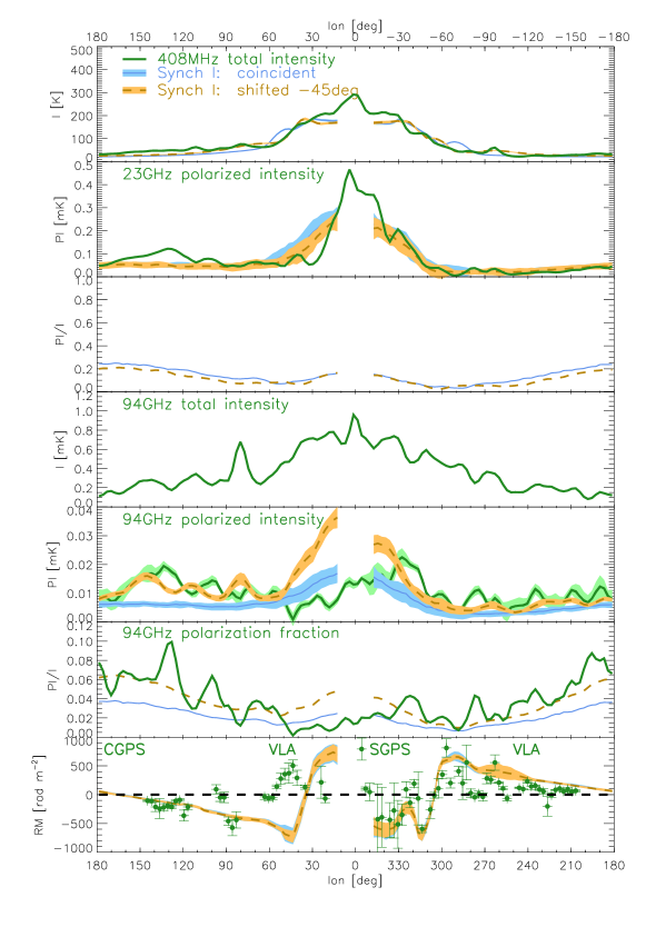
Figure 2: Panels as in Fig. 1. The blue line is the model from Fig. 1 and has coincident arms for all components while the dashed yellow model is that where the isotropic random field component has been shifted back 45$\degr$ in Galactic azimuth, as shown in Fig. 3. See § 5.

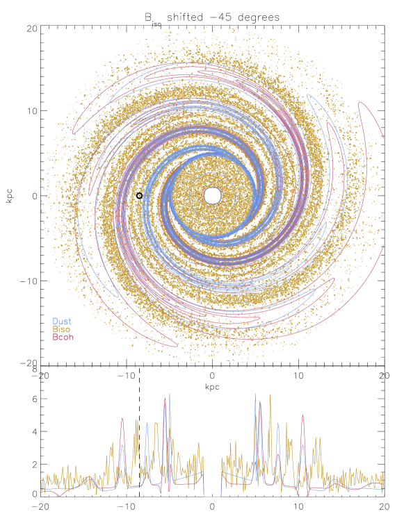
Figure 3: Top panel: contour plot of the Galaxy model seen from above. The magenta traces the coherent and ordered random magnetic fields. In blue is the dust distribution. In gold is the isotropic random field component. The Sun position is at -8.5 kpc, to the left of the galactic centre. The lower panel shows the profile on the axis connecting the Sun and the Galactic centre. The observed profiles along the plane are shown in Fig. 2.

5.4 Comparison to low-frequency radio polarisation

Note that the model in Fig. 3 has the Sun position (8.5 kpc to the left of centre) just inside the isotropic random field arm. This means that looking toward the outer Galaxy, we ought to see Faraday depolarisation effects in the low-frequency radio data in that direction. Though the strength of the depolarisation effect is unknown and would require some additional modeling to estimate, it is clear that the effect is the opposite of what is seen, namely that it is the inner Galaxy where there is significant Faraday depolarisation and the outer Galaxy only where strong polarisation is apparent. See, e.g., fig. 1 of Burigana et al. (2006) showing the polarised emission at 1.4 GHz. The implication is that the positions of the arms in our model may need to be adjusted relative to the position of the Sun.

We will in future add to our studies the Faraday depolarisation effects seen in the 1.4 GHz polarisation map, since this is important additional data on the spatial distribution of the turbulent medium.

6 Discussion

We show in Section 5 how the profiles of polarised synchrotron and dust emission in the Galactic plane, combined with previous work to constrain average strengths of the field components in the Galaxy, require a spatial separation of the different field components. It is clear from Fig. 2 that a constant mixing of the coherent plus ordered random fields with the isotropic random component is inconsistent with the polarised dust data in the Galactic plane. We can also see that the problem is opposite in the inner and outer Galaxy. Our current model cannot simultaneously fit both regions, but we can already draw some conclusions from Fig. 2.

6.1 The shock scenario

Firstly, we can reproduce the emission in the outer Galaxy with a model where the isotropic random component peaks in arms that are clearly separated from both the coherent and ordered random components and the dust emitting regions. The synchrotron emission constrains only the average amount of coherent plus ordered random and isotropic random magnetic fields in the Galaxy, but does not strongly depend on where they are located. External galaxies show indications of magnetic arms distinct from the gas arms and with morphologies that are not necessarily the same (see, e.g., Frick et al. 2000 or Beck 2009). They can be shifted relative to each other, have different pitch angles, or cross over the gas arm ridges. There is clear evidence for such effects in the case of M51 (Patrikeev et al., 2006). Our results in the outer Galaxy support the idea of a shift between components.

The second conclusion we can draw from Fig. 2 is that the situation is reversed in the inner Galaxy, where the data show no peak in the polarised emission as predicted, implying that the fields are less ordered in the dust emitting regions than in our models. Our current model cannot be tuned to simultaneously fit both regions.

We can reproduce the polarisation in the outer Galaxy with a model that has the peak of dust emission spatially coincident with the coherent and ordered random fields but offset from the isotropic random field. Such a lag can be naturally explained by the idea of a large-scale shock wave associated with the spiral arm: the shock compresses the fields so they lie predominantly parallel to the shock, compresses the gas and dust likewise, and triggers collapse of dust clouds and subsequently star formation. The turbulence is then generated in supernovae downstream of the compression after the stars have had time to evolve, thus explaining the shift in the isotropic random field component relative to the other arms.

This scenario is also consistent with the studies by Haverkorn et al. (2006, 2008), which examine the structure function of Faraday RM fluctuations in directions either tangent to spiral arms or tangent to inter-arm regions. They find that in the inter-arm regions, the structure function shows a rising spectrum up to a cut-off scale, consistent with turbulence from a Kolmogorov cascade of energies from large scale turbulence injected by supernova remnants. The arm tangents by contrast do not show such a spectrum but rather a flat structure function, perhaps implying a much smaller outer scale of turbulence, small enough that the turn-over on the structure function is not visible. This is interpreted by Haverkorn et al. as an alternative source of turbulence, e.g. HII regions and stellar winds instead of supernova remnants. But it is also what one might expect to see if the larger scale turbulence has been compressed perpendicular to the shock, i.e. perpendicular to the LOS when looking tangent to the arms. Alternatively, it could simply be that the the star formation is triggered in the shock and only later evolves into the supernova remnants that inject the turbulence, which would mean the turbulence is always downstream of the compressed region.

Since the downstream region is leading the shock inside co-rotation (where the interstellar gas rotates faster than the spiral pattern) and lagging behind the shock outside co-rotation, our simple model of spiral arms being azimuthally shifted as wholes is not accurate. The value of the co-rotation radius is very uncertain (e.g., Gerhard 2011), but it could be close to the Galacto-centric radius of the Sun, in which case inner/outer Galaxy would roughly coincide with inside/outside co-rotation. In other words, the depolarising turbulence would be shifted ahead of the dust arms in the inner Galaxy, and behind the dust arms in the outer Galaxy. But this difference in the shift direction would not change the polarisation degree.

It should be noted that the dust is emitted mostly in relatively compact clouds that are not resolved by our simulations. One can easily imagine different degrees of ordering in the magnetic fields in the clouds compared to the diffuse ISM traced by synchrotron emission, e.g. by turbulence injected at smaller scales. As discussed in § 4.4, however, our modeling effectively assumes 30 per cent polarization at the scale of a typical cloud, which is significantly higher than anything observed. Furthermore, there is also a truly diffuse dust component that would trace the large-scale turbulence seen in synchrotron emission, though the ratio of such emission to that from relatively compact clouds is unknown. We therefore find it difficult to envision a plausible alternative scenario to increase the dust polarization in the outer Galaxy as long as the dust clouds remain embedded in the same turbulent ISM that is traced by the synchrotron.

6.2 Refinements for the inner Galaxy

There are several possibilities that might explain the difference in the inner Galaxy. Broadly speaking, they are either that the dust-emitting regions have more disordered fields in the inner Galaxy, or that the intrinsic polarisation fraction of the dust emission drops.

We could perhaps model the former by allowing the field components to have different pitch angles so that the isotropic random component is coincident with the dust in the inner Galaxy but gradually shifts away in the outer Galaxy. This would result in a degree of ordering that would vary with Galacto-centric radius and might be made to reproduce the data. But this would not be consistent with the shock compression scenario that naturally accounts for the polarisation in the outer Galaxy, and we currently lack a plausible alternative scenario for such a morphology.

There is similarly a question of when the collapsing dust clouds decouple from the magnetic fields. There is more star formation in the inner Galaxy, and the colder dusty regions could be less strongly coupled to the large-scale ordered fields in the inner Galaxy. Even if the clouds remain coupled to the fields while collapsing, the collapse itself could disrupt the ordering in the fields. Since the synchrotron emission comes from a large volume while the dust emission may be dominated by relatively isolated regions of collapsing clouds, the dust emitting regions may have more random fields at small scales embedded in the larger-scale fields traced by synchrotron.

Alternatively, the truly intrinsic polarisation fraction could drop in the inner Galaxy due to the different environment (e.g. temperature) of the dusty regions. As discussed in § 4.4, the intrinsic polarisation fraction is not well understood.

We could fold these possibilities into an effective sub-grid polarisation fraction that varies with Galacto-centric radius. Our large-scale analysis cannot distinguish these possibilities without additional external constraints on small-scale dust polarization properties, but higher-resolution studies of the fields in individual clouds may be very informative.

6.3 Caveats

Note that the uncertainty in the true intrinsic polarisation fraction of dust does not affect our analysis in the outer Galaxy. As discussed in § 4.4, it is very unlikely to be high enough to account for the observed polarisation without spatially separating the dust from the isotropic random fields.

Another uncertainty in this analysis is the impact of the possible modulation of the CRE density due to the two effects discussed in § 4.3, namely the compression and acceleration of the CREs at the spiral-arm shocks and the distribution of CRE injection sites. Both sources of CRE density modulation arise in spiral arms, but they are not necessarily spatially coincident, as CREs are presumably injected by supernova remnants in the turbulent regions that develop downstream from the shocks, away from the amplified fields. One can speculate that the two effects may result in a fairly uniform average CRE density across spiral arms, thus explaining the observed lack of any such modulation in the CRE density.

In order to reproduce the observed level of synchrotron emission, and not to result in arm tangents that are more peaked in emission than observed, any CRE enhancement would have to be offset by a corresponding lowering of the coherent and ordered random magnetic fields. In any case, the degree of polarisation of the dust emission does not depend on the strength of the fields, only on the degree of ordering in the dusty regions. So the question of the CRE density is an interesting one but does not have a large effect on our main conclusions.

Neither the uncertainty in the intrinsic polarisation fraction of dust emission nor in the CRE density modulation, therefore, will change our main conclusion: that in the outer Galaxy, the dust emitting regions have more ordered fields than the average as traced by synchrotron emission.

7 Conclusions

We have continued our project to model the large scale Galactic magnetic fields by adding the polarised thermal dust emission from the WMAP 94 GHz band. We find that our model previously fit to synchrotron and Faraday RMs does not reproduce the observed level of dust polarisation. Even with an assumed intrinsic polarisation fraction of 30 per cent, which is higher than observed, the level of predicted polarisation is too low in all but the innermost regions of the Galactic plane. This implies that the dust emitting regions have more ordered magnetic fields than average. We are able to reproduce the data in the outer Galaxy by modifying the model to spatially separate the isotropic random field component from the dust emitting regions and the coherent and ordered random field components. This separation is consistent with the scenario of fields and dust compressed in the spiral arm shocks, with turbulence generated by supernova remnants downstream. The same model results in an over-prediction of the dust polarisation in the inner regions of the Galaxy, which indicates that a more sophisticated model is necessary. We will in further work explore models that allow either the spiral arm characteristics of each component or the dust intrinsic polarisation degree to vary with Galacto-centric radius. Our models would be improved by numerical simulations of galaxies’ magnetic fields that included arm versus inter-arm variations and provided constraints to break some of our parameter degeneracies. This project will be significantly aided by the Planck satellite’s more sensitive observations of polarised dust emission at both large and small scales.

Appendix A Model parametrization

The following tables describe the parametrization of the magnetic field and dust distribution models. The difference to previous works is in simplifying the radial profiles (since we do not fit the innermost region of the Galaxy where the Broadbent (1989) features have effect) and in making the field continuous in the transitions between arms. Each component has an associated scale height, which is unconstrained by our analysis confined to the Galactic plane. But they are given for completeness and for the small effect they may have within the resolution of 6$\degr$.

Total field $\mathbf{B}_{\mathrm{tot}}=\mathbf{B}_{\mathrm{coh}}+\mathbf{B}_{\mathrm{iso}}+\mathbf{B}_{\mathrm{ord}}$
Param.	Default	Equation	Description
Axisymmetric spiral coherent magnetic field: $\mathbf{B}_{\mathrm{ASS}}(r,\phi,z)=B(r)B_{\mathrm{coh}}(z)\mathbf{\hat{B}}$
$B_{0}$	1 $\upmu$G		Global amplitude normalisation
$R_{\mathrm{scale}}$	20 kpc	$B(r)=B_{0}\exp(-r^{2}/R_{\mathrm{scale}}^{2})$	Outer radial profile parameter. See fig. 3 of Jaffe et al. (2010).
$h_{\mathrm{g}}$	6 kpc	$B_{\mathrm{coh}}(z)=\mathrm{sech}^{2}(z/h_{\mathrm{g}})$	Global scale height of the coherent field.
$R_{\mathrm{max}}$	20 kpc		Maximum radius, beyond which $|B|=0$
$R_{\mathrm{mol}}$	5 kpc	$\mathbf{\hat{B}}=\left\{\begin{array}[]{ll}(\cos(\phi+\pi/2)\mathbf{\hat{e}}_{x},\sin(\phi+\pi/2)\mathbf{\hat{e}}_{y},0)&\mbox{ if $r\leq R_{\mathrm{mol}}$ }\\ (\sin(\theta_{p})\mathbf{\hat{e}}_{r},\cos(\theta_{p})\mathbf{\hat{e}}_{\phi},0)&\mbox{ if $r>R_{\mathrm{mol}}$ }\\ \end{array}\right.$	Field direction circular within “molecular ring” and otherwise spiral (expressed in cylindrical coordinates, with the x-axis between the Sun and Galactic centre).
$\theta_{p}$	-11.5$\degr$		$\theta_{p}$ is the pitch angle of field direction and spiral arms
Spiral compression arm coherent magnetic field: $\mathbf{B}_{\mathrm{coh}}=\mathbf{B}_{\mathrm{ASS}}+\sum_{i}^{N_{\mathrm{arms}}}\mathbf{B}_{\mathrm{arm},i}$
$a_{i}$	$(3,0.5,-4,$$1.2,-0.8)$	$\mathbf{B}_{\mathrm{arm},i}=B(r)a_{i}\rho_{c}(d_{i})\mathbf{\hat{B}}$	Amplitude of each of four spiral arms and molecular ring..
		$\rho_{c}(d)=c(r)B_{\mathrm{comp}}(z)\exp(-(d/d_{0}(r))^{2})$	Additional compression factor relative to background. $d$ is the distance to the nearest arm in kpc, computed using $r_{i}(\phi)$
$\phi_{0,i}$	$10\degr+90\degr i$	$r_{i}(\phi)=R_{s}\exp\left[(\phi-\phi_{0,i})/\beta\right]$ and $\beta\equiv 1/\tan(\theta_{p})$	$r(\phi)$ gives arm radius at given azimuth, and $\phi_{0,i}$ the azimuthal orientation of the rotation of spiral around axis through Galactic poles
$R_{\mathrm{comp}}$	7.1 kpc		Scale radius of compressed spiral arms.
$C_{0}$	2.5	$c(r)=\left\{\begin{array}[]{ll}C_{0}&\mbox{ if $r\leq r_{\mathrm{cc}}$ }\\ C_{0}(r/r_{\mathrm{cc}})^{-3}&\mbox{ if $r>r_{\mathrm{cc}}$ }\\ \end{array}\right.$	Arm compression amplitude, tailing off after a region of constant compression. The contrast, $\epsilon\equiv n^{\mathrm{(d)}}/n^{\mathrm{(u)}}$, is the ratio of downstream (post-shock) to upstream (pre-shock) density, in which case $C_{0}\approx\epsilon-1$ if we consider arm versus inter-arm instead of down- versus upstream.)
$r_{\mathrm{cc}}$	12 kpc	See $c(r)$.	Region of constant compression.
$d_{0}$	0.3 kpc	$d_{0}(r)=d_{0}/(c(r)B(r))$	Defines the base width of arm enhancement, which varies with radius.
$h_{\mathrm{c}}$	2 kpc	$B_{\mathrm{comp}}(z)=\mathrm{sech}^{2}(z/h_{\mathrm{c}})$	Scale height of the spiral compression.
Isotropic random and ordered random magnetic fields:
$\mathbf{B}_{\mathrm{iso}}+\mathbf{B}_{\mathrm{ord}}=\left[\mathbf{B}_{\mathrm{GRF}}B_{\mathrm{GRF}}(z)B_{\mathrm{GRF}}(r)+\sum_{i}^{N}\mathbf{B}_{\mathrm{arm},i}^{\mathrm{iso}}\right]+\sum_{i}^{N}\mathbf{B}_{\mathrm{arm},i}^{\mathrm{ord}}$
$h_{\mathrm{r}ms}$	2 kpc	$B_{\mathrm{GRF}}(z)=\mathrm{sech}^{2}(z/h_{\mathrm{r}ms})$	Global scale height of the turbulent field field.
$R_{\mathrm{G}RF}$	20 kpc	$B_{\mathrm{GRF}}(r)=\exp(-r^{2}/R^{2}_{\mathrm{G}RF})$	Global scale radius of the turbulent field.
$\alpha$	-0.37	$P_{B}(k)\equiv\left<|{\bf B}_{\mathrm{GRF}}(k)|^{2}\right>\propto k^{\alpha}$ and                        ${\bf B}_{\mathrm{GRF}}({\bf x})=\mathcal{F}^{-1}\left[{\bf B}_{\mathrm{GRF}}({\bf k})\right]$	Power law spectral index of initial GRF; default of -0.37 from Han et al. (2004) in 1D (compare to 3D Kolmogorov turbulence prediction of $-5/3$).
$D_{\mathrm{co}}$	0.1 kpc	$B_{\mathrm{GRF}}(k)=0$ for $k<1/D_{\mathrm{co}}$	Cutoff maximum of GRF fluctuations (minimum determined by resolution)
$B_{\mathrm{rms}}$	3.5	$B_{\mathrm{rms}}\equiv\left<B_{\mathrm{GRF}}^{2}({\bf x})\right>^{1/2}$	Total RMS amplitude of GRF fluctuations
$f_{\mathrm{ord}}$	0.15	${\bf B}_{\mathrm{arm,i}}^{\mathrm{iso}}=\rho_{c}{\bf B}_{\mathrm{GRF}}$ and ${\bf B}_{\mathrm{arm,i}}^{\mathrm{ord}}=f_{\mathrm{ord}}\rho_{c}{\bf B}_{\mathrm{proj}}$	Relates ordered to isotropic random component. $\bf{B}_{\mathrm{proj}}$ is the component of the GRF parallel to the coherent field direction, i.e. the spiral.

Table 2: Table of magnetic field modelling parameters as described in § 3.1. The total field is the sum of the coherent, isotropic random, and ordered random components. The coherent and isotropic random each have a (statistically) axisymmetric and a spiral component, while the ordered random only has the spiral component. Parameter values for the spiral are the same for each component in this work with the exception of $C_{0}$, which in Fig. 2 is different for the isotropic random component only.

Dust emissivity model parameters:
Parameter	Default	Description
$h_{\mathrm{g,d}}$	0.4 kpc	Scale height of dust uncompressed component.
$h_{\mathrm{c,d}}$	0.1 kpc	Scale height of the dust arms.
$R_{\mathrm{scale,d}}$	8 kpc	Scale radius of the uncompressed component.
$R_{\mathrm{comp,d}}$	13 kpc	Scale radius of the compressed spiral arms.
$C_{0,\mathrm{d}}$	6	Compression factor for dust.
$d_{0,\mathrm{d}}$	0.1 kpc	Base width of dust arms. The width varies with $r$ as described in Table 2.

Table 3: Table of parameters for the dust density distribution. The parametrization is the same as for the magnetic field models defined in Table 2, an axisymmetric component plus a spiral compressed component, and any parameters not listed here are the same.

References

- Abdo et al. (2009) Abdo A. A. et al., 2009, Physical Review Letters, 103, 251101
- Abdo et al. (2010) Abdo A. A. et al., 2010, The Astrophysical Journal, 710, 133
- Ackermann et al. (2010) Ackermann M. et al., 2010, Physical Review D, 82, 92004
- Ackermann et al. (2011) Ackermann M. et al., 2011, The Astrophysical Journal, 726, 81
- Beck (2009) Beck R., 2009, Proc. IAU Symposium, 259, pp 3–14
- Benoît et al. (2004) Benoît A. et al., 2004, Astronomy and Astrophysics, 424, 571
- Broadbent (1989) Broadbent A., 1989, (PhD thesis, Durham Univ.)
- Broadbent et al. (1990) Broadbent A., Haslam C. G. T., Osborne J. L., 1990, in Proceedings of the 21st International Cosmic Ray Conference. Volume 3 (OG Sessions). p. 229
- Brown et al. (2007) Brown J. C., Haverkorn M., Gaensler B. M., Taylor A. R., Bizunok N. S., McClure-Griffiths N. M., Dickey J. M., Green A. J., 2007, ApJ, 663, 258
- Brown et al. (2003) Brown J. C., Taylor A. R., Jackel B. J., 2003, ApJS, 145, 213
- Burigana et al. (2006) Burigana C., La Porta L., Reich P., Reich W., 2006, Astronomische Nachrichten, 327, 491
- Cordes & Lazio (2002) Cordes J. M., Lazio T. J. W., 2002, preprint (astro-ph/0207156)
- Dickinson et al. (2003) Dickinson C., Davies R. D., Davis R. J., 2003, MNRAS, 341, 369
- Draine & Fraisse (2009) Draine B. T., Fraisse A. A., 2009, The Astrophysical Journal, 696, 1
- Drimmel & Spergel (2001) Drimmel R., Spergel D. N., 2001, ApJ, 556, 181
- Effenberger et al. (2012) Effenberger F., Fichtner H., Scherer K., Buesching I., 2012, astro-ph/1210.1423
- Fauvet et al. (2011) Fauvet L. et al., 2011, Astronomy and Astrophysics, 526, 145
- Fauvet et al. (2012) Fauvet L., Macías-Pérez J. F., Jaffe T. R., Banday A. J., Désert F. X., Santos D., 2012, Astronomy and Astrophysics, 540, 122
- Fletcher et al. (2011) Fletcher A., Beck R., Shukurov A., Berkhuijsen E., Horellou C., 2011, Monthly Notices of the Royal Astronomical Society, 412, 2396
- Frick et al. (2000) Frick P., Beck R., Shukurov A., Sokoloff D., Ehle M., Kamphuis J., 2000, Monthly Notices of the Royal Astronomical Society, 318, 925
- Gerhard (2002) Gerhard O., 2002, in Proceedings. p. 73
- Gerhard (2011) Gerhard O., 2011, Memorie della Societa Astronomica Italiana Supplementi, 18, 185
- Górski et al. (2005) Górski K. M., Hivon E., Banday A. J., Wandelt B. D., Hansen F. K., Reinecke M., Bartelmann M., 2005, ApJ, 622, 759
- Han et al. (2004) Han J. L., Ferriere K., Manchester R. N., 2004, ApJ, 610, 820
- Haslam et al. (1982) Haslam C. G. T., Stoffel H., Salter C. J., Wilson W. E., 1982, A&AS, 47, 1
- Haverkorn et al. (2008) Haverkorn M., Brown J. C., Gaensler B. M., McClure-Griffiths N. M., 2008, The Astrophysical Journal, 680, 362
- Haverkorn et al. (2006) Haverkorn M., Gaensler B. M., Brown J. C., Bizunok N. S., McClure-Griffiths N. M., Dickey J. M., Green A. J., 2006, The Astrophysical Journal, 637, L33
- Jaffe et al. (2011) Jaffe T. R., Banday A. J., Leahy J. P., Leach S., Strong A. W., 2011, Monthly Notices of the Royal Astronomical Society, 416, 1152
- Jaffe et al. (2010) Jaffe T. R., Leahy J. P., Banday A. J., Leach S. M., Lowe S. R., Wilkinson A., 2010, Monthly Notices of the Royal Astronomical Society, 401, 1013
- Jansson & Farrar (2012) Jansson R., Farrar G. R., 2012, ApJ, 757, 14
- Jansson et al. (2009) Jansson R., Farrar G. R., Waelkens A. H., Enßlin T. A., 2009, Journal of Cosmology and Astro-Particle Physics, 7, 21
- Jarosik et al. (2011) Jarosik N. et al., 2011, The Astrophysical Journal Supplement, 192, 14
- Landau & Lifshitz (1987) Landau Lifshitz 1987, Fluid Mechanics. Vol. 6
- Lorimer et al. (2006) Lorimer D. R. et al., 2006, Monthly Notices of the Royal Astronomical Society, 372, 777
- Northrop (1963) Northrop T., 1963, The adiabatic motion of charged particles
- Patrikeev et al. (2006) Patrikeev I., Fletcher A., Stepanov R., Beck R., Berkhuijsen E. M., Frick P., Horellou C., 2006, Astronomy and Astrophysics, 458, 441
- Planck Collaboration (2011) Planck Collaboration 2011, A&A, 536, A1
- Ponthieu et al. (2005) Ponthieu N. et al., 2005, Astronomy and Astrophysics, 444, 327
- Stern (1966) Stern D. P., 1966, Space Science Reviews, 6, 147
- Strong et al. (2010) Strong A., Porter T., Digel S., Jóhannesson G., Martin P., Moskalenko I., Murphy E., Orlando E., 2010, The Astrophysical Journal Letters, 722, L58
- Strong et al. (2011) Strong A. W., Orlando E., Jaffe T. R., 2011, Astronomy and Astrophysics, 534, 54
- Sun et al. (2008) Sun X. H., Reich W., Waelkens A., Enßlin T. A., 2008, A&A, 477, 573
- van Eck et al. (2011) van Eck C. et al., 2011, ApJ, 728, 97
- Waelkens et al. (2009) Waelkens A., Jaffe T., Reinecke M., Kitaura F. S., Enßlin T. A., 2009, A&A, 495, 697