Observational constraints on non-minimally coupled Galileon model

Abstract

Abstract: As an extension of Dvali-Gabadadze-Porrati (DGP) model, the Galileon theory has been proposed to explain the “self-accelerating problem” and “ghost instability problem”. In this Paper, we extend the Galileon theory by considering a non-minimally coupled Galileon scalar with gravity. The statefinder analysis, $Om(z)$ diagnostic and constraint the model parameters have been investigate , we find $\Omega_{\text{m0}}=0.263_{-0.031}^{+0.031}$, $n=1.53_{-0.37}^{+0.21}$ (at the $95\%$ confidence level) with $\chi^{2}_{\text{min}}=473.376$. Further we show that due to the SNe Ia + BAO data ,our model behaves like a phantom-like dark energy.

I Introduction

The observational data can be use to probe the the equation of state (EoS) of dark energy $w_{\rm X}$ using the Supernovae Ia (SNe Ia) data SNearly , Cosmic Microwave Background radiations (CMB) CMBearly and Baryon Acoustic Oscillations (BAO) BAO1 ; Percival:2009xn .

Over the past decade,different kinds of the dynamical dark energy models have been discussed (see Refs. review for review). Some popular models are like quintessence quin , $f(R)$gravity fR , scalar field models stensor , the Dvali-Gabadadze-Porrati (DGP) braneworld DGP scenario,modified gravities Tsujikawa:2010zza , the Gauss-Bonnet gravity fG , $f(R,{\cal G})$ gravity fRG ,$f(R,T)$ gravity (Here $T$ is the trace of the energy-momentum tensor), frt ; ft and so on. Physically we need to find an effective gravitational action, which can recover the Einstein gravity Will . These modifications must be free from any extra degree of freedoms due to the ghostDeFelice ; DGPghost . In modified $f(R)$ theory and it’s reduction to scalar field models, we need to be careful in picking the mathematical forms of $f(R)$ or the field potentials functions in order to have compatibility with astrophysical observations fRviable . The scalar mode of the DGP theory is due to a longitudinal mode of a free massless sping 2 graviton with self interaction $\square\phi(\partial^{\mu}\phi\partial_{\mu}\phi)$ which is the mixing with the transverse gravitonDGPnon . The physical mechanism which is hidden behind such decoupling is so-called by Vainshtein mechanism Vainshtein . It means that it is possible to recover the Einstein gravity in a region of spacetime in size of the solar scales. The graviton interaction term of the form $\square\phi(\partial^{\mu}\phi\partial_{\mu}\phi)$ satisfies the non-Lorentzian invariance form of the classical boost symmetry, resembles the Galilean local boost transformation

$$\nabla_{\mu}\phi\rightarrow\nabla_{\mu}\phi+c_{\mu},$$

in the flat space-time. The non relativistic model, based on the Galilean symmetry called as the “Galileon” Nesseris:2010pc . It has been shown that there are only five field Lagrangians ${\cal L}_{i}$ ($i=1,\cdots,5$) which are invariant under the Galilean symmetry. Their discussion was based on the Minkowski background. The equation of the motion (EOM) derived from this action is second-order. Consequently, the model seems free from extra unphysical degenerated modes. The plan of this Paper is the following: In section II, we introduce our proposed model of non-minimal Galileon cosmology. In section III, we perform the statefinder and Om diagnostics on model. In section IV, we discuss the observational constraints on our model. In section V, we provide the Conclusion of our Paper.

II Non-minimal Galileon Cosmology

The covariant Galileon action reads Nesseris:2010pc

$$\mathcal{S}=\int{\rm d}^{4}x\sqrt{-g}\,\left[\frac{1}{2\kappa^{2}}(1-\epsilon\kappa^{2}\xi\pi^{2})R+\frac{1}{2}\sum_{i=1}^{5}c_{i}{\cal L}_{i}\right]+\int{\rm d}^{4}x\,{\cal L}_{M}\,,$$ (1)

with $g$ as $det(g_{\mu\nu})$ in units of $\kappa^{2}=8\pi G$, and the Galileon coupling constants $c_{i}$ are constants. The covariant Lagrangians ${\cal L}_{i}$ ($i=1,\cdots,5$) are given by Nesseris:2010pc

$${\cal L}_{1}=M^{3}\pi\,,\quad{\cal L}_{2}=(\nabla\pi)^{2}\,,\quad{\cal L}_{3}=(\square\pi)(\nabla\pi)^{2}/M^{3}\,,$$

$${\cal L}_{4}=(\nabla\pi)^{2}\left[2(\square\pi)^{2}-2\pi_{;\mu\nu}\pi^{;\mu\nu}-R(\nabla\pi)^{2}/2\right]/M^{6},$$

$${\cal L}_{5}=(\nabla\pi)^{2}[(\square\pi)^{3}-3(\square\pi)\,\pi_{;\mu\nu}\pi^{;\mu\nu}$$

$$~{}~{}~{}~{}~{}~{}~{}+2{\pi_{;\mu}}^{\nu}{\pi_{;\nu}}^{\rho}{\pi_{;\rho}}^{\mu}-6\pi_{;\mu}\pi^{;\mu\nu}\pi^{;\rho}G_{\nu\rho}]/M^{9}\,,$$ (2)

where $M$ is the mass parameter of Galileon model. Using the following standard metric

$${\rm d}s^{2}=-{\rm d}t^{2}+a^{2}(t)\left[\frac{{\rm d}r^{2}}{1-Kr^{2}}+r^{2}({\rm d}\theta^{2}+\sin^{2}\theta\,{\rm d}\phi^{2})\right]\,,$$ (3)

the equations of motion read

$$3H^{2}=\kappa^{2}(\rho_{\rm DE}+\rho_{m}+\rho_{r}+\rho_{K}+\rho_{\xi})\,,$$ (4)

$$3H^{2}+2\dot{H}=-\kappa^{2}(P_{\rm DE}+\rho_{r}/3+\rho_{K}/3+P_{\xi})\,,$$ (5)

$$\dot{\rho}_{m}+3H\rho_{m}=0\,,$$ (6)

$$\dot{\rho}_{r}+4H\rho_{r}=0\,,$$ (7)

where

$$\rho_{\xi}=6\xi\epsilon\pi H\dot{H}+3\xi\epsilon\pi^{2}H^{2},$$ (8)

$$P_{\xi} = \frac{\epsilon}{2}(1-4\xi)\dot{\pi}^{2}+2\epsilon\xi\dot{\pi}-2\epsilon\xi(1-6\xi)\dot{H}\pi^{2}$$

$$-3\xi\epsilon(1-8\xi)H^{2}\pi^{2}-\frac{1}{2}c_{1}\xi\pi.$$

and $\rho_{K}\equiv-3K/a^{2}\kappa^{2}$.

$$\rho_{\rm DE} \equiv -c_{1}M^{3}\pi/2-c_{2}\dot{\pi}^{2}/2+3c_{3}H\dot{\pi}^{3}/M^{3}$$ (10)

$$-45c_{4}H^{2}\dot{\pi}^{4}/(2M^{6})+21c_{5}H^{3}\dot{\pi}^{5}/M^{9},$$

$$P_{\rm DE} \equiv c_{1}M^{3}\pi/2-c_{2}\dot{\pi}^{2}/2-c_{3}\dot{\pi}^{2}\ddot{\pi}/M^{3}$$ (11)

$$+3c_{4}\dot{\pi}^{3}[8H\ddot{\pi}+(3H^{2}+2\dot{H})\dot{\pi}]/(2M^{6})$$

$$-3c_{5}H\dot{\pi}^{4}[5H\ddot{\pi}+2(H^{2}+\dot{H})\dot{\pi}]/M^{9}\,.$$

The solutions of (6) and (7) are respectively given by

$$\rho_{\text{m}}=\rho_{\text{m0}}a^{-3},\ \ \rho_{\text{r}}=\rho_{\text{r0}}a^{-4}.$$ (12)

We must write (5) in the following form

$$(H^{2})^{\prime}=-\kappa^{2}\Big{(}\rho_{\rm DE}+P_{\rm DE}+\frac{4}{3}\rho_{m}+\rho_{\xi}+P_{\xi}\Big{)},$$ (13)

in this new representation the deprivates are written with respect to the e-folding $\mathcal{N}=\ln a$. Figure 1 shows the time evolutionary scheme of the metric and the Galileon gauges, numerically. Also, the agreement of the Hubble parameter in our model and LCDM model is obviously manifested from the right panel.

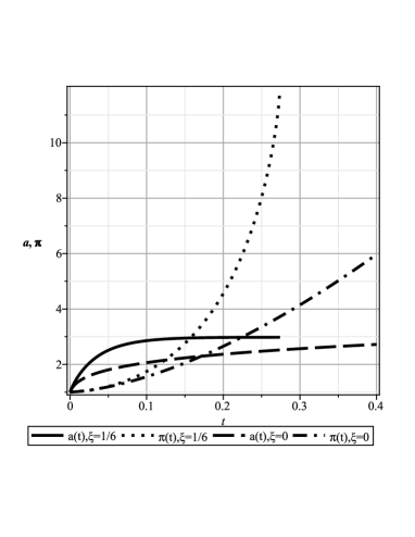
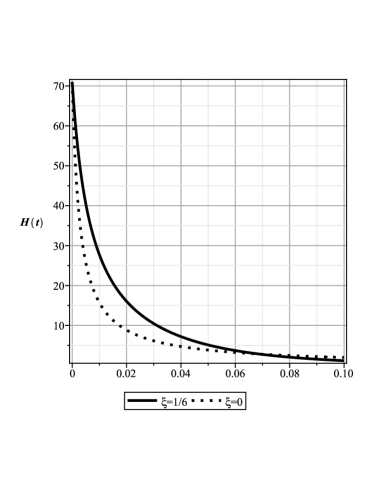
Figure 1: (Left) Time evolution of scale factor $a(t)$ and Galileon scalar $\pi$. (Right) Time evolution of the Hubble parameter $H(t)$.

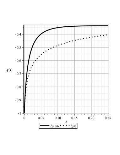
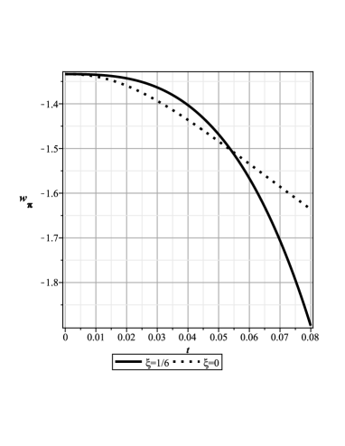
Figure 2: (Left) Deceleration parameter $q$. (Right) Equation of state parameter $w_{\pi}$.

III Statefinder Analysis and $Om$ Diagnostic

In order to classify the different dark energy models, Sanhi et al. Sanhi proposed a geometrical diagnostic method by considering higher derivatives of the scale factor. The statefinder parameters $\{r,s\}$ are defined

$$r\equiv\frac{\dddot{a}}{aH^{3}}\;,$$ (14)

$$s\equiv\frac{r-1}{3(q-1/2)}\;,$$ (15)

where $q\equiv-\frac{1}{H^{2}}\frac{\ddot{a}}{a}$ is the deceleration parameter. Apparently, $\Lambda$CDM model corresponds to a point $\{1,0\}$ in $\{r,s\}$ phase space. The statefinder diagnostic can discriminate different models. For example, it can distinguish quintom from other dark energy models WuYu . From the panel of figure-1, we observe that behavior of Hubble parameter can be approximated as

$$H\propto\frac{1}{t^{n}},\ \ n\geq 1.$$ (16)

With this ansatz form, the behavior of statefinder parameters is

$$r=\frac{n^{2}-3n+2}{n^{2}},\ \ s=\frac{2(3n-2)t^{n}}{3n(nt^{n}-2)}.$$ (17)

For very far future $t\rightarrow\infty$,

$$r=1-\frac{3n-2}{n^{2}},\ \ s=\frac{2(3n-2)}{3n^{2}},$$ (18)

which can be combined as

$$r=1-\frac{3s}{2}.$$ (19)

From (16), the scale factor evolves like

$$a(t)=a_{0}\exp\Big{(}\frac{t^{1-n}-t_{0}^{1-n}}{1-n}\Big{)}.$$ (20)

From this expression we obtain the Hubble parameter $H(z)$:

$$H(z)=H_{0}\Big{[}1+t_{0}^{n-1}(n-1)\log(1+z)\Big{]}^{\frac{n}{n-1}}.$$ (21)

We assume that $t_{0}=1$. So, the parameter for our model is $n$. Indeed, $n=n(\xi)$. We interpolate

$$n(\xi)=\Sigma_{m=1}^{5}c_{m}\xi^{m},\ \ \xi\in\textit{Z}.$$ (22)

It is very interesting to investigate the behavior of the (20) in limit of the limit $n\rightarrow 1$. In this case for (20) we have

$$a(t)=a_{0}\Big{(}\frac{t}{t_{0}}\Big{)},\ \ H(t)=\frac{1}{t}.$$ (23)

The $Om(z)$ is another diagnostic of dark energy proposed by Sahni et al. Sahni2008 . It is defined as

$$Om(z)\equiv\frac{E^{2}(z)-1}{(1+z)^{3}-1}.$$ (24)

By defining $E^{2}=H^{2}/H^{2}_{0}$. Obviously, this diagnostic parameter depends only to the first derivative of the luminosity distance $D_{L}(z)$. We are able from this diagnostic to discriminate different dark energy models by interpolating the geometrical slope of $Om(z)$ although we don’t know the precise value of $\Omega_{\text{m0}}$. The figure 2 shows different graphs of the deceleration parameter and effective EoS by indicating the DE behavior in the phantom era. Also the statefinder analysis has been presented in the figure 3.

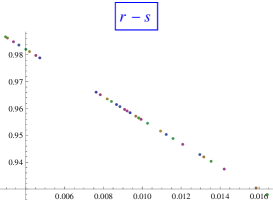
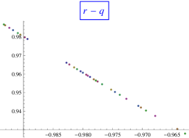
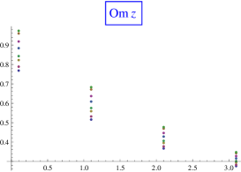
Figure 3: The evolutionary curves of statefinder pair $(r,s)$ (left), pair $(r,q)$ (middle) and $Om(z)$ (right) for (21) with $\Omega_{\text{m0}}=0.278$, $-1<z<4$. Here we plot for $1.2<n<1.5$ and $0.67<\xi<0.82$

IV Observational Constraints

We will now discuss the constraints on our model parameter $n$ which appeared in (21) with (13). Here we perform the data analysis using SNe Ia, BAO and SDSS Amanullah2010 . First we must review these data sets (see Appendix A of Wu:2010mn for a review).
In (2010), the Supernova Cosmology Project collaboration  Amanullah2010 reported the Union2 compilation, which consists of 557 SNe Ia data points. In fact this is the largest reported and spectroscopically confirmed SNe Ia sample . We use it to constrain the theoretical models in this paper based on the model (5). As usually, the results can be obtained by minimizing the $\hat{\chi}^{2}$

$$\hat{\chi}^{2}_{Sne}=\sum_{i=1}^{557}\frac{[\mu_{obs}(z_{i})-\mu_{th}(z_{i})]^{2}}{\sigma_{u,i}^{2}}\;,$$ (25)

where $\sigma_{\mu,i}^{2}$ are the errors . The luminosity distance $D_{L}$ can be calculated by Eisenstein2005 ; Nesseris2005

$$D_{L}\equiv(1+z)\int_{0}^{z}\frac{dz^{\prime}}{E(z^{\prime})}.\;$$ (26)

Calculating the ${\chi}^{2}_{SNe}$, we find that, the best fit values are $\Omega_{\text{m0}}=0.271$, $n=n(\xi)=1.52$ with $\chi^{2}_{Min}=481.272$. The results has been in figure 4 for different confidence limits.

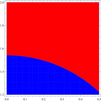
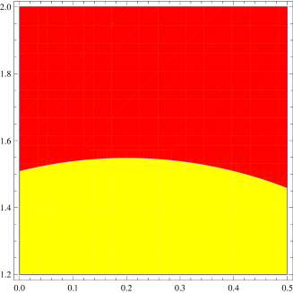
Figure 4: The $1\sigma$ and $2\sigma$ contours for $(\Omega_{\text{m0}},n)$ parameter space arising from the Sne Ia + BAO. The constraints on Model (21) from Sne Ia + BAO. The regions corresponds to $1-\sigma$ (Blue-left), $2-\sigma$ (Yellow-right) confidence regions. Here Red is the background color.

Now, using BAO data. The parameter $A$ represented using the BAO peak Eisenstein2005 . The constraints from SNe Ia+BAO are given by minimizing $\chi^{2}_{SNe}+\chi^{2}_{BAO}$. The results are $\Omega_{\text{m0}}=0.263_{-0.031}^{+0.031}$, $n=1.53_{-0.37}^{+0.21}$ (at the $95\%$ confidence level) with $\chi^{2}_{\text{min}}=473.376$.

V Conclusions

We constrained a non-minimally coupled Galileon gravity with Lagrangian $\mathcal{L}=\frac{1}{2\kappa^{2}}(1-\epsilon\kappa^{2}\xi\pi^{2})R+\frac{1}{2}\sum_{i=1}^{5}c_{i}{\cal L}_{i}$. Compared with references, we examine our model with SNe Ia+BAO data . Using SNe Ia and BAO, we find that the exponent power of Hubble parameter $n=\Sigma_{i=1}^{5}c_{m}\xi^{m}\approx 1.5$, which contains the CDM model. We like to mention here that we have followed largely the exposition given in the Wu and Yu paper wuyu1 .

References

- (1) A. G. Riess et al., Astron. J. 116, 1009 (1998); Astron. J. 117, 707 (1999); S. Perlmutter et al., Astrophys. J. 517, 565 (1999).
- (2) D. N. Spergel et al., Astrophys. J. Suppl. 148, 175 (2003); D. N. Spergel et al. [WMAP Collaboration], Astrophys. J. Suppl. 170, 377 (2007).
- (3) D. J. Eisenstein et al. [SDSS Collaboration], Astrophys. J. 633, 560 (2005).
- (4) W. J. Percival et al., Mon. Not. Roy. Astron. Soc. 401, 2148 (2010).
-
(5)
V. Sahni and A. A. Starobinsky,
Int. J. Mod. Phys. D 9, 373 (2000);
M. Jamil, D. Momeni, N. S. Serikbayev, R. Myrzakulov, Astrophys
Space Sci 339, 37 (2012);
M. Jamil, Y. Myrzakulov, O. Razina, R. Myrzakulov, Astrophys Space Sci 336, 315 (2011);
M. Jamil, S. Ali, D. Momeni and R. Myrzakulov, Eur. Phys. J. C 72, 1998 (2012) [arXiv:1201.0895 [physics.gen-ph]]. -
(6)
Y. Fujii, Phys. Rev. D 26, 2580 (1982);
L. H. Ford, Phys. Rev. D 35, 2339 (1987);
C. Wetterich, Nucl. Phys B. 302, 668 (1988); -
(7)
S. Nojiri and S. D. Odintsov,
Phys. Rept. 505, 59 (2011)
[arXiv:1011.0544 [gr-qc]];
S. Capozziello, V.F. Cardone, A. Troisi, JCAP 0608, 001 (2006);
S. Capozziello, V.F. Cardone, A. Troisi, Mon. Not. Roy. Astron. Soc. 375, 1423 (2007);
C. Frgerio Martins and P. Salucci, Mon. Not. Roy. Astron. Soc. 381, 1103 (2007);
G. Cognola, et al., Phys. Rev. D 77, 046009 (2008);
R. Myrzakulov, D. S.-G mez, A. Tureanu, Gen.Rel.Grav.43:1671-1684,2011;
E. Elizalde, R. Myrzakulov, V. V. Obukhov, D. S.-G mez,Class.Quant.Grav.27:095007,2010;
M. Cvetic, S. Nojiri, S.D. Odintsov, Nucl.Phys.B628:295-330,2002. A. Azadi, D. Momeni, M. Nouri-Zonoz, Phys.Lett.B670:210-214(2008);
D. Momeni, H. Gholizade , Int.J.Mod.Phys.D18,1719(2009);
M. Jamil, F. M. Mahomed, D. Momeni, Phys.Lett.B702,315(2011);
S. H. Hendi, D. Momeni, Eur. Phys. J. C 71 ,1823 (2011);
M. Sharif, H. Rizwana Kausar, J. Phys. Soc. Jpn. 80,044004(2011);
S. H. Hendi, B. Eslam Panah, S. M. Mousavi, Gen Relativ Gravit, 44,835 (2012);
M. Farasat Shamir, Astrophys. Space Sci.330,183(2010);
M. Sharif, M. Farasat Shamir, Class.Quant.Grav.26,235020(2009);
T. R. P. Caram s, E. R. Bezerra de Mello, Eur. Phys.J. C 64:113-121, (2009);
M.R. Setare, M. Jamil, Gen. Relativ. Gravit. (2011) 43:293-303 - (8) M. Jamil, S. Ali, D. Momeni, R. Myrzakulov, Eur. Phys. J. C 72, 1998 (2012); L. Amendola, Phys. Rev. D 60, 043501 (1999); J. P. Uzan, Phys. Rev. D 59, 123510 (1999); T. Chiba, Phys. Rev. D 60, 083508 (1999); N. Bartolo and M. Pietroni, Phys. Rev. D 61, 023518 (2000); F. Perrotta, C. Baccigalupi and S. Matarrese, Phys. Rev. D 61, 023507 (2000); A. Aslam, M. Jamil, D. Momeni and R. Myrzakulov, arXiv:1212.6022 [astro-ph.CO].
- (9) G. R. Dvali, G. Gabadadze and M. Porrati, Phys. Lett. B 485, 208 (2000); G. R. Dvali, G. Gabadadze and M. Porrati, Phys. Lett. B 485, 208 (2000).
- (10) S. Tsujikawa, Lect. Notes Phys. 800, 99 (2010) [arXiv:1101.0191 [gr-qc]].
- (11) S. Nojiri, S. D. Odintsov and M. Sasaki, Phys. Rev. D 71, 123509 (2005); T. Koivisto and D. F. Mota, Phys. Lett. B 644, 104 (2007); Phys. Rev. D 75, 023518 (2007); S. Tsujikawa and M. Sami, JCAP 0701, 006 (2007); A. De Felice and S. Tsujikawa, Phys. Lett. B 675, 1 (2009); Phys. Rev. D 80, 063516 (2009); M.R. Setare, M. Jamil, Europhys.Lett.92:49003,2010.
-
(12)
S. M. Carroll et al.,
Phys. Rev. D 71, 063513 (2005);
I. Navarro and K. Van Acoleyen, Phys. Lett. B 622, 1 (2005);
JCAP 0603, 008 (2006);
A. De Felice and T. Suyama, JCAP 0906, 034 (2009); Phys. Rev. D 80, 083523 (2009);
A. De Felice, J. M. Gerard and T. Suyama, Phys. Rev. D 82, 063526 (2010);
M. Jamil, D. Momeni and M. A. Rashid, Eur. Phys. J. C 71, 1711 (2011) [arXiv:1107.1558 [physics.gen-ph]];
D. Momeni, Int. J. Theor. Phys. 50, 1493 (2011) [arXiv:0910.0594 [gr-qc]];
M. R. Setare and D. Momeni, Int. J. Mod. Phys. D 19, 2079 (2010) [arXiv:0911.1877 [hep-th]];
A. De Felice and T. Tanaka, Prog. Theor. Phys. 124, 503 (2010);
E. Elizalde, R. Myrzakulov, V. V. Obukhov, D. S ez-G mez, Class.Quant.Grav,27,095007(2010);
M. E. Rodrigues, M. J. S. Houndjo, D. Momeni and R. Myrzakulov, arXiv:1212.4488 [gr-qc]; M. J. S. Houndjo, M. E. Rodrigues, D. Momeni and R. Myrzakulov, arXiv:1301.4642 [gr-qc]. -
(13)
M. Jamil, D. Momeni, M. Raza, R. Myrzakulov, Eur. Phys. J. C 72,1999 (2012);
M. J. S. Houndjo, F. G. Alvarenga, Manuel E. Rodrigues, Deborah F. Jardim, arXiv:1207.1646 [gr-qc];
T. Azizi, arXiv:1205.6957[gr-qc]; F. G. Alvarenga, M. J. S. Houndjo, A. V. Monwanou, Jean B. Chabi Orou, arXiv:1205.4678 [gr-qc] . -
(14)
M. J. S. Houndjo, D. Momeni, R. Myrzakulov,Int.J.Mod.Phys. D21 (2012) 1250093, arXiv:1206.3938 ;
M. Jamil, D. Momeni, R. Myrzakulov,Eur. Phys. J. C ,72,1959 (2012);
K.K.Yerzhanov, Sh.R.Myrzakul, I.I.Kulnazarov, R.Myrzakulov, arXiv:1006.3879 ;
M. Jamil, D. Momeni, R. Myrzakulov, Eur. Phys. J. C 72, 2122 (2012);
M. Jamil, D. Momeni, R. Myrzakulov, Eur. Phys. J. C 72, 2075 (2012);
K. Bamba, R. Myrzakulov, S. Nojiri, S. D. Odintsov, Phys. Rev. D 85, 104036 (2012);
M. Jamil, D. Momeni, R. Myrzakulov, Eur. Phys. J. C 73, 2267 (2013);
M. Jamil, D. Momeni, R. Myrzakulov, Gen. Relativ. Grav. 45, 263 (2013);
M. Jamil, D. Momeni, R. Myrzakulov, P. Rudra, J. Phys. Soc. Jpn. 81, 114004 (2012);
M. Jamil, D. Momeni, R. Myrzakulov, Eur. Phys. J. C 72, 2137 (2012);
R. Myrzakulov, Eur. Phys. J. C 71, 1752 (2011);
K. Bamba, M. Jamil, D. Momeni, R. Myrzakulov, Astrophysics and Space Science, DOI :10.1007/s10509-012-1312-2,arXiv:1202.6114 . - (15) C. M. Will, Living Rev. Rel. 4, 4 (2001); Living Rev. Rel. 9, 3 (2005); B. Bertotti, L. Iess and P. Tortora, Nature 425, 374 (2003).
- (16) A. De Felice, M. Hindmarsh and M. Trodden, JCAP 0608, 005 (2006); G. Calcagni, B. de Carlos and A. De Felice, Nucl. Phys. B 752, 404 (2006).
- (17) M. A. Luty, M. Porrati and R. Rattazzi, JHEP 0309, 029 (2003); A. Nicolis and R. Rattazzi, JHEP 0406, 059 (2004); K. Koyama and R. Maartens, JCAP 0601, 016 (2006); D. Gorbunov, K. Koyama and S. Sibiryakov, Phys. Rev. D 73, 044016 (2006).
-
(18)
K. Bamba, A. Lopez-Revelles, R. Myrzakulov, S. D. Odintsov and L. Sebastiani,
arXiv:1301.3049 [gr-qc];
S. A. Appleby and R. A. Battye, Phys. Lett. B 654, 7 (2007). -
(19)
C. Deffayet, G. R. Dvali, G. Gabadadze and A. I. Vainshtein,
Phys. Rev. D 65, 044026 (2002);
M. Porrati, Phys. Lett. B 534, 209 (2002). - (20) A. I. Vainshtein, Phys. Lett. B 39, 393 (1972).
- (21) S. Nesseris, A. De Felice and S. Tsujikawa, Phys. Rev. D 82, 124054 (2010) [arXiv:1010.0407 [astro-ph.CO]].
- (22) V. Sahni, T. D. Saini, A. A. Starobinsky and U. Alam, ETP Lett. 77, 201 (2003) [Pisma Zh. Eksp. Teor. Fiz. 77, 249 (2003)]; V. Sahni, A. Shafieloo and A. A. Starobinsky, Phys. Rev. D 78, 103502 (2008).
- (23) P. Wu and H. W. Yu, Phys. Lett. B 693, 415 (2010) [arXiv:1006.0674 [gr-qc]].
- (24) P. Wu and H. Yu, Int. J. Mod. Phys. D 14, 1873 (2005).
- (25) V. Sahni, A. Shafieloo and A. A. Starobinsky, Phys. Rev. D 78, 103502 (2008).
- (26) R. Amanullah, et al., arXiv:1004.1711.
- (27) D. J. Eisenstein, et al., Astrophys. J. 633, 560 (2005).
- (28) S. Nesseris and L. Perivolaropoulos, Phys. Rev. D 72, 123519 (2005).
- (29) P. Wu, H. Yu, Eur. Phys. J. C 71, 1552 (2011).