A Bayesian nonparametric approach to modeling market share dynamics

Abstract

We propose a flexible stochastic framework for modeling the market share dynamics over time in a multiple markets setting, where firms interact within and between markets. Firms undergo stochastic idiosyncratic shocks, which contract their shares, and compete to consolidate their position by acquiring new ones in both the market where they operate and in new markets. The model parameters can meaningfully account for phenomena such as barriers to entry and exit, fixed and sunk costs, costs of expanding to new sectors with different technologies and competitive advantage among firms. The construction is obtained in a Bayesian framework by means of a collection of nonparametric hierarchical mixtures, which induce the dependence between markets and provide a generalization of the Blackwell–MacQueen Pólya urn scheme, which in turn is used to generate a partially exchangeable dynamical particle system. A Markov Chain Monte Carlo algorithm is provided for simulating trajectories of the system, by means of which we perform a simulation study for transitions to different economic regimes. Moreover, it is shown that the infinite-dimensional properties of the system, when appropriately transformed and rescaled, are those of a collection of interacting Fleming–Viot diffusions.

and

1 Introduction

The idea of explaining firm dynamics by means of a stochastic model for the market evolution has been present in the literature for a long time. However, only recently, firm-specific stochastic elements have been introduced to generate the dynamics. Jovanovic [26] was the first to formulate an equilibrium model where stochastic shocks are drawn from a distribution with known variance and firm-specific mean, thus determining selection of the most efficient. Later Ericson and Pakes [12] provide a stochastic model for industry behavior which allows for heterogeneity and idiosyncratic shocks, where firms invest and the stochastic outcome determines the firm’s success, thus accounting for a selection process which can lead to the firm’s exit from the market. Hopenhayn [24] performs steady state analysis of a dynamic stochastic model which allows for entry, exit and heterogeneity. In [38] a stochastic model for market share dynamics, based on simple random walks, is introduced. The common feature of this non-exhaustive list is that, despite the mentioned models being inter-temporal and stochastic, the analysis and the explicit description of the model dynamics are essentially done at equilibrium, thus projecting the whole construction onto a static dimension and accounting for time somehow implicitly. Indeed, the researcher usually finds herself before the choice between a dynamic model with a representative agent and a steady-state analysis of an equilibrium model with heterogeneity. Furthermore, relevant for our discussion are two technical difficulties with reference to devising stochastic models for market share dynamics: the interdependence of market shares, and the fact that the distribution of the size of shocks to each firm’s share is likely to depend on that firm’s current share. As stated in [38], these together imply that an appropriate model might be one in which the distribution of shocks to each firm’s share is conditioned on the full vector of market shares in the current period.

The urge to overcome these problems from an aggregate perspective, while retaining the micro dynamics, has lead to a recent tendency of borrowing ideas from statistical physics for modeling certain problems in economics and finance. A particularly useful example of these tools is given by interacting particle systems, which are arbitrary-dimensional models describing the dynamic interaction of several variables (or particles). These allow for heterogeneity and idiosyncratic stochastic features but still permit a relatively easy investigation of the aggregate system properties. In other words, the macroscopic behavior of the system is derived from the microscopic random interactions of the economic agents, and these techniques allow us to keep track of the whole tree of outcomes in an inter-temporal framework. A recent example of such an approach is given in [5], where interacting particle systems are used to model the propagation of financial distress in a network of firms. Another example is [36], which studies limit theorems for the process of empirical measures of an economic model driven by a large system of agents that interact locally by means of mechanisms similar to what, in population genetics, are called mutation and recombination.

Here we propose a Bayesian nonparametric approach for modeling market share dynamics by constructing a stochastic model with interacting particles which allows us to overcome the above mentioned technical difficulties. In particular, a nonparametric approach allows us to avoid any unnecessary assumption on the distributional form of the involved quantities, while a Bayesian approach naturally incorporates probabilistic clustering of objects and features conditional predictive structures, easily admitting the representation of agents’ interactions based on the current individual status. Thus, with respect to the literature on market share dynamics, we model time explicitly, instead of analyzing the system at equilibrium, while retaining heterogeneity and conditioning on the full vector of market shares. And despite the different scope, with respect to the particles approach in [36], we instead consider many subsystems with interactions among each other and thus obtain a vector of dependent continuous-time processes. In constructing the model, the emphasis will be on generality and flexibility, which necessarily implies a certain degree of stylization of the dynamics. However, this allows the model to be easily adapted to represent diverse applied frameworks, such as, for example, population genetics, by appropriately specifying the corresponding relevant parameters. As a matter of fact, we will follow the market share motivation throughout the paper, with the parallel intent of favoring intuition behind the stochastic mechanisms. A completely micro-founded economic application will be provided in a follow-up paper [32]. However, besides the construction, the present paper includes an asymptotic distributional result which shows weak convergence of the aggregate system to a collection of dependent diffusion processes. This is a result of independent mathematical interest, relevant, in particular, for the population genetics literature, where our construction can be seen as a countable approximation of a system of Fleming–Viot diffusions with mutation, selection and migration (see [6]). Appendix A includes some basic material on Fleming–Viot processes.

Finally, it is worth mentioning that our approach is also allied to recent developments in the Bayesian nonparametric literature: although structurally different, our model has a natural interpretation within this field as belonging to the class of dependent processes, an important line of research initiated in the seminal papers of [30, 31]. Among others, we mention interesting dependent models developed in [9, 10, 11, 35, 39] where one can find applications to epidemiology, survival analysis and functional data analysis. See the monograph [23] for a recent review of the discipline. Although powerful and flexible, Bayesian nonparametric methods have not yet been extensively exploited for economic applications. Among the contributions to date, we mention [33, 27, 22] for financial time series, [21, 19] for volatility estimation, [28] for option pricing and [3, 8] for discrete choice models, [20] for stochastic frontier models. With respect to this literature, the proposed construction can be seen as a dynamic partially exchangeable array, so that the dependence is meant both with respect to time and in terms of a vector of random probability measures.

To be more specific, we introduce a flexible stochastic model for describing the time dynamics of the market concentration in several interacting, self-regulated markets. A potentially infinite number of companies operate in those markets where they have a positive share. Firms can enter and exit a market, and expand or contract their share in competition with other firms by means of endogenous stochastic idiosyncratic shocks. The model parameters allow for barriers to entry and exit, costs of expansion in new markets (e.g., technology conversion costs), sunk costs and different mechanisms of competitive advantage. The construction is achieved by first defining an appropriate collection of dependent nonparametric hierarchical models and deriving a related system of interacting generalized Pòlya urn schemes. This underlying Bayesian framework is detailed in Section 2. The collection of hierarchies induces the dependence between markets and allows us to construct, in Section 3, a dynamic system, which is driven by means of Gibbs sampling techniques [18] and describes how companies interact among one another within and between markets over time. These undergo stochastic idiosyncratic shocks that lower their current share and compete to increment it. An appropriate set of parameters regulates the mechanisms through which firms acquire and lose shares and determines the competitive selection in terms of relative strengths as functions of their current position in the market and, possibly, the current market configuration as a whole. For example, shocks can be set to be random in general but deterministic when a firm crosses upwards some fixed threshold, meaning that some antitrust authority has fixed an upper bound on the market percentage which can be controlled by a single firm, which is thus forced away from the dominant position. The competitive advantage allows for a great degree of flexibility, involving a functional form with very weak assumptions. In Section 4 the dynamic system is then mapped into a measure-valued process, which pools together the local information and describes the evolution of the aggregate markets. The system is then shown to converge in distribution, under certain conditions and after appropriate rescaling, to a system of dependent diffusion processes, each with values in the space of probability measures, known as interacting Fleming–Viot diffusions. In Section 5 two algorithms which generate sample paths of the system are presented, corresponding to competitive advantage directly or implicitly modeled. A simulation study is then performed to explore dynamically different economic scenarios with several choices of the model parameters, investigating the effects of changes in the market characteristics on the economic dynamics. Particular attention is devoted to transitions of economic regimes as dependent on specific features of the market, on regulations imposed by the policy maker or on the interaction with other markets with different structural properties. Finally, Appendix A briefly recalls some background material on Gibbs sampling, Fleming–Viot processes and interacting Fleming–Viot processes, while all proofs are deferred to Appendix B.

2 The underlying framework

In this section we define a collection of dependent nonparametric hierarchical models, which will allow a dynamic representation of the market’s interaction.

Let $\alpha$ be a finite non-null measure on a complete and separable space $\mathbb{X}$ endowed with its Borel sigma algebra $\mathscr{X}$, and consider the Pòlya urn for a continuum of colors, which represents a fundamental tool in many constructions of Bayesian nonparametric models. This is such that $X_{1}\sim\alpha(\cdot)/\alpha(\mathbb{X})$, and, for $n\geq 2$,

$$X_{n}|X_{1},\ldots,X_{n-1}\sim\frac{\alpha(\cdot)+\sum_{i=1}^{n-1}\delta_{X_{k}}(\cdot)}{\alpha(\mathbb{X})+n-1},$$ (1)

where $\delta_{y}$ denotes a point mass at $y$. We will denote the joint law of a sequence $(X_{1},\ldots,X_{n})$ from (1) with $\mathcal{M}_{n}^{\alpha}$, so that

$$\mathcal{M}_{n}^{\alpha}=\frac{\alpha}{\alpha(\mathbb{X})}\prod_{i=2}^{n}\frac{\alpha+\sum_{k<i}\delta_{X_{k}}}{\alpha(\mathbb{X})+i-1}.$$ (2)

In [2] it is shown that this prediction scheme is closely related to the Dirichlet process prior, introduced by [16]. A random probability measure $P$ on $(\mathbb{X},\mathscr{X})$ is said to be a Dirichlet process with parameter measure $\alpha$, henceforth denoted $P\sim\mathscr{D}(\cdot|\alpha)$, if for every $k\geq 1$ and every measurable partition $B_{1},\ldots,B_{k}$ of $\mathbb{X}$, the vector $(P(B_{1}),\ldots,P(B_{k}))$ has Dirichlet distribution with parameters $(\alpha(B_{1}),\ldots,\alpha(B_{k}))$.

Among the various generalizations of the Pòlya urn scheme (1) present in the literature, a recent extension given in [37] will be particularly useful for our construction. Consider, for every $n\geq 1$, the joint distribution

$$q_{n}(\mathrm{d}x_{1},\ldots,\mathrm{d}x_{n})\propto p_{n}(\mathrm{d}x_{1},\ldots,\mathrm{d}x_{n})\prod_{k=1}^{n}\beta_{n}(x_{k}),$$ (3)

where $\beta_{n}$ is a given bounded measurable function on $\mathbb{X}$. A representation for (3) can be provided in terms of a Dirichlet process mixture model [29]. In particular, it can be easily seen that when $p_{n}\equiv\mathcal{M}_{n}^{\alpha}$ in (3), the predictive distribution for $X_{i}$, given $\mathbf{x}_{(-i)}=(x_{1},\ldots,x_{i-1},x_{i+1},\ldots,x_{n})$, is

$$q_{n,i}\bigl{(}\mathrm{d}x_{i}|\mathbf{x}_{(-i)}\bigr{)}\propto\beta_{n}(x_{i})\alpha(\mathrm{d}x_{i})+\sum_{k\neq i}^{n}\beta_{n}(x_{i})\delta_{x_{k}}(\mathrm{d}x_{i}).$$ (4)

This can be thought of as a weighted version of (1), which is recovered when $\beta_{n}\equiv 1$ for all $n\geq 1$. A more general version of (4) can be obtained by making $\beta_{n}$ depend on the whole vector and thus allowing for a broad range of interpretations. See the discussion following (3) for this and for a more detailed interpretation of (4) in the context of the present paper.

Consider now the following setting. For each $n$, let $(X_{1},\ldots,X_{n})\in\mathbb{X}^{n}$ be an $n$-sized sample from $\mathcal{M}_{n}^{\alpha}$, and let

$$\alpha_{x_{1},\ldots,x_{n}}(\mathrm{d}y)=\alpha(\mathrm{d}y)+\sum_{k=1}^{n}\delta_{x_{k}}(\mathrm{d}y).$$ (5)

Define the double hierarchy

$$X_{1},\ldots,X_{n}|P \stackrel{{\scriptstyle\mathrm{i.i.d.}}}{{\sim}} P,\qquad P\sim\mathscr{D}(\cdot|\alpha),$$

$$Y_{1},\ldots,Y_{n}|Q_{n} \stackrel{{\scriptstyle\mathrm{i.i.d.}}}{{\sim}} Q_{n},\qquad Q_{n}\sim\mathscr{D}(\cdot|\alpha_{x_{1},\ldots,x_{n}}).$$

Here $(X_{1},\ldots,X_{n})$ are drawn from a Dirichlet process $P\sim\mathscr{D}(\cdot|\alpha)$ and $(Y_{1},\ldots,Y_{n})$, given $(X_{1},\ldots,X_{n})$, are drawn from a Dirichlet process $Q_{n}:=Q|(X_{1},\ldots,X_{n})\sim\mathscr{D}(\cdot|\alpha_{X_{1},\ldots,X_{n}})$. It can be easily seen that the joint law of $(Y_{1},\ldots,Y_{n})$ conditional on $(X_{1},\ldots,X_{n})$ is $\mathcal{M}_{n}^{\alpha_{x_{1},\ldots,x_{n}}}$, with $\mathcal{M}_{n}^{\alpha}$ as in (2). The following result, stated here for ease of reference, can be found in [41].

Lemma 2.1.

Let $\mathcal{M}_{n}^{\alpha}$ be as in (2). Then

$$\int_{\mathbb{X}^{n}}\mathcal{M}_{n}^{\alpha_{x_{1},\ldots,x_{n}}}(\mathrm{d}y_{1},\ldots,\mathrm{d}y_{n})\mathcal{M}_{n}^{\alpha}(\mathrm{d}x_{1},\ldots,\mathrm{d}x_{n})=\mathcal{M}_{n}^{\alpha}(\mathrm{d}y_{1},\ldots,\mathrm{d}y_{n}).$$ (7)

In particular, Lemma 2.1 yields a certain symmetry in (2), so that we could also state that the joint law of $(X_{1},\ldots,X_{n})$ conditional on $(Y_{1},\ldots,Y_{n})$ is $\mathcal{M}_{n}^{\alpha_{y_{1},\ldots,y_{n}}}$. Denote $\mathbf{x}=(x_{1},\ldots,x_{n})$ and extend (3) to

$$q_{n}(\mathrm{d}\mathbf{x})\propto p_{n}(\mathrm{d}\mathbf{x})\prod_{k=1}^{n}\beta_{n}(x_{k}),\qquad q_{n}(\mathrm{d}\mathbf{y})\propto p_{n}(\mathrm{d}\mathbf{y})\prod_{k=1}^{n}\beta_{n}(y_{k}).$$

From (4), when $(X_{1},\ldots,X_{n})$ and $(Y_{1},\ldots,Y_{n})$ come from (2) we have for $1\leq i\leq n$

$$q_{2n,i}\bigl{(}\mathrm{d}x_{i}|\mathbf{x}_{(-i)},\mathbf{y}\bigr{)}\propto\beta_{n}(x_{i})\alpha_{y_{1},\ldots,y_{n}}(\mathrm{d}x_{i})+\sum_{k\neq i}^{n}\beta_{n}(x_{k})\delta_{x_{k}}(\mathrm{d}x_{i})$$ (8)

and similarly for $y_{i}$. It is now straightforward to iterate the above argument and allow for an arbitrary number of dependent hierarchies. Denote $\mathbf{x}^{r}=(x^{r}_{1},\ldots,x^{r}_{n})$ and $\alpha_{\mathbf{x}^{r}}=\alpha_{x^{r}_{1},\ldots,x^{r}_{n}}$, where $r,r^{\prime},r^{\prime\prime}$ belong to some finite index set $\mathcal{I}$, whose cardinality is denoted $\#\mathcal{I}$. Then, for every $n\geq 1$, let

$$\begin{array}[]{rcl@{ \qquad}rcl}\mathbf{X}^{r}|P&\stackrel{{\scriptstyle\mathrm{i.i.d.}}}{{\sim}}&P,&P&\sim&\mathscr{D}(\cdot|\alpha),\\ \vspace*{5pt}\cr\mathbf{X}^{r}|P^{r}&\stackrel{{\scriptstyle\mathrm{i.i.d.}}}{{\sim}}&P^{r},&P^{r}&\sim&\mathscr{D}(\cdot|\alpha_{\mathbf{x}^{r}}),\\ \vspace*{5pt}\cr\mathbf{X}^{r^{\prime\prime}}|P^{r^{\prime},r^{\prime\prime}}&\stackrel{{\scriptstyle\mathrm{i.i.d.}}}{{\sim}}&P^{r^{\prime},r^{\prime\prime}},&P^{r^{\prime},r^{\prime\prime}}&\sim&\mathscr{D}(\cdot|\alpha_{\mathbf{x}^{r},\mathbf{x}^{r^{\prime}}}),\\ \vspace*{5pt}\cr&\vdots&&&\vdots&\end{array}$$ (13)

where the dimension subscript $n$ has been suppressed in $\mathbf{X}^{r},\mathbf{X}^{r^{\prime}},\mathbf{X}^{r^{\prime\prime}},\ldots,$ for notational simplicity. Denote now with

$$D_{n}=n\cdot\#\mathcal{I}$$ (14)

the total number of components in (13). The joint law of the $D_{n}$ items in (13) can be written

$$\mathcal{M}_{n}^{\alpha}(\mathrm{d}\mathbf{x}^{r})\mathcal{M}_{n}^{\alpha_{\mathbf{x}^{r}}}(\mathrm{d}\mathbf{x}^{r^{\prime}})\mathcal{M}_{n}^{\alpha_{\mathbf{x}^{r},\mathbf{x}^{r^{\prime}}}}(\mathrm{d}\mathbf{x}^{r^{\prime\prime}})\cdots,$$ (15)

where, in view of Lemma 2.1, (15) is invariant with respect to the order of $r,r^{\prime},r^{\prime\prime},\ldots.$ With a slight abuse of notation, define

$$\mathcal{I}(-r)=\{\mathbf{x}^{r^{\prime}}\colon\ r^{\prime}\in\mathcal{I},r^{\prime}\neq r\},$$ (16)

to be the set of all system components without the vector $\mathbf{x}^{r}$, and

$$\mathcal{I}(-x^{r}_{i})=\{\mathbf{x}^{r^{\prime}}\colon\ r^{\prime}\in\mathcal{I}\}\setminus\{x^{r}_{i}\}$$ (17)

to be the set of all system components without the item $x_{i}^{r}$. Analogously to (8) in this enlarged framework, the predictive law for $x^{r}_{i}$, conditional on the rest of the system, can be written

$$q_{{}_{D_{n},i}}(\mathrm{d}x^{r}_{i}|\mathcal{I}(-x^{r}_{i}))\propto\beta_{n}(x^{r}_{i})\alpha_{{}_{\mathcal{I}(-r)}}(\mathrm{d}x^{r}_{i})+\sum_{k\neq i}^{n}\beta_{n}(x^{r}_{k})\delta_{x^{r}_{k}}(\mathrm{d}x^{r}_{i}),$$ (18)

where the interpretation of $\alpha_{{}_{\mathcal{I}(-r)}}$ is clear from (5) and (16). Note that this predictive law reduces to (1) when $\beta_{n}\equiv 1$ and $\alpha_{{}_{\mathcal{I}(-r)}}\equiv\alpha$. Expression (18) will be the key for the definition of the market dynamics by means of an interacting system of particles. A detailed interpretation for $q_{D_{n},i}$ will be provided in the following section. See (3) and the following discussion.

To conclude the section, it is worth noting that (13) generates a partially exchangeable array, where partial exchangeability is intended in the sense of de Finetti (see, e.g., [4]). That is, if $r,r^{\prime},r^{\prime\prime}$ identify rows, then the system components are row-wise exchangeable but not exchangeable.

3 Dynamic models for market evolution

In this section we define a dynamical model for the temporal evolution of the firms’ market shares in multiple interacting markets. The model can be regarded as a random element whose realizations are right-continuous functions from $[0,\infty)$ to the space $(\mathbb{X}^{D_{n}},\mathscr{X}^{D_{n}})$, $D_{n}\in\mathbb{N}$ being (14), and we refer to it as a particle system, since it explicitly models the evolution of the share units, or particles, in several markets. For ease of presentation, we approach the construction by first considering a single market for a fixed number $n$ of share units, and then extend it to a collection of markets. The investigation of the asymptotic properties as $n\rightarrow\infty$ is, instead, the object of Section 4.

For any fixed $n\geq 1$, consider a vector $\mathbf{x}=\mathbf{x}^{(n)}=(x_{1},\ldots,x_{n})\in\mathbb{X}^{n}$, and let $(x_{1}^{*},\ldots,x_{K_{n}}^{*})$ denote the $K_{n}\leq n$ distinct values in $\mathbf{x}$, with $x_{j}^{*}$ having multiplicity $n_{j}$. The elements of $(x_{1}^{*},\ldots,x_{K_{n}}^{*})$ represent the $K_{n}$ firms operating in the market at a given time. Here $x_{j}^{*}$ is a random label to be seen as a unique firm identifier. The vector $\mathbf{x}$ represents the current market configuration, carrying implicitly the information on the shares. Namely, the fraction of elements in $\mathbf{x}$ equal to $x_{j}^{*}$ is the market share possessed by firm $j$. Here $n$ represents the level of share fractionalization in the market. Dividing the market into $n$ fractions is not restrictive, since any share can be approximated by means of a sufficiently large $n$. See Remark 5.1 below for a discussion of the implications of this assumption on the computational costs.

Define now a Markov chain taking values in $\mathbb{X}^{n}$ as follows. At each step an index $i$ is chosen from $\{1,\ldots,n\}$ with probability $\gamma_{n,i}\geq 0$ for $i=1,\ldots,n$, with $\sum_{i=1}^{n}\gamma_{n,i}=1$. Equivalently, let $\gamma_{j}(\mathbf{n}_{n})$ be the probability that firm $x_{j}^{*}$ loses an $n$th fraction of its market share at a certain transition, where $\gamma_{j}(\mathbf{n}_{n})$ depends on the frequencies $\mathbf{n}_{n}=(n_{1},\ldots,n_{K_{n}})$. That is, firm $x_{j}^{*}$ undergoes a shock whose probability is idiosyncratic, depending on the firm itself and on the current market configuration, summarized by the vector of frequencies. Different choices of $\gamma_{j}(\mathbf{n}_{n})$ reflect different market regulations, possibly imposed by the policy maker. We provide some examples:

1. [(3)]

2. $\gamma_{j}(\mathbf{n}_{n})=1/K_{n}$: neutrality. All firms have equal probability of undergoing a shock;

3. $\gamma_{j}(\mathbf{n}_{n})=n_{j}/n$: firms with higher shares are the weakest, with a flattening effect on the share distribution. This parametrization is also useful in population genetics contexts, where particles represent individuals;

4. $\gamma_{j}(\mathbf{n}_{n})=(1-n_{j}/n)/(K_{n}-1)$ when $K_{n}\geq 2$: firms with higher shares are the strongest. The probability of losing shares is decreasing in the firms’ positions in the market;

5. $\gamma_{j}(\mathbf{n}_{n})=\mathbf{1}(\max_{i}n_{i}\leq nC)\tilde{\gamma}_{j}(\mathbf{n}_{n})+\mathbf{1}(n_{j}>nC)$ for some constant $0<C<1$, where $\mathbf{1}(A)$ is the indicator function of the event $A$. The probability of selecting $x_{j}^{*}$ is $\tilde{\gamma}_{j}(\mathbf{n}_{n})$ provided no firm controls more than $C\%$ of the market. If firm $x_{j}^{*}$ controls more than $C\%$ of the market, at the following step, $x_{j}^{*}$ is selected with probability one. Thus $C$ is an upper bound imposed by the policy maker to avoid dominant positions. Incidentally, there is a subtler aspect of this mechanism which is worth commenting upon. It will be seen later that there is positive probability that the same firm acquires the vacant share again, but this only results in picking again $x_{j}^{*}$ with probability one, until the threshold $C$ is crossed downwards. This seemingly anomalous effect can be thought of as the viscosity with which a firm in a dominant position gets back to a legitimate status when condemned by the antitrust authority, which in no real world occurs instantaneously.

Suppose now $x_{i}=x_{j}^{*}$ has been chosen in $\mathbf{x}$. Once firm $x_{j}^{*}$ looses a fraction of its share, the next state of the chain is obtained by sampling a new value for $X_{i}$ from (4), leaving all other components unchanged. Hence the $i$th fraction of share is reallocated, according to the predictive distribution of $X_{i}|\mathbf{x}_{(-i)}$, either to an existing firm or to a new one entering the market.

Remark 3.1.

The above Markov chain can also be thought of as generated by a Gibbs sampler on $q_{n}(\mathrm{d}x_{1},\ldots,\mathrm{d}x_{n})$. This consists of sequentially updating one randomly selected component at a time in $(x_{1},\ldots,x_{n})$ according to the component-specific full conditional distribution $q_{n,i}(\mathrm{d}x_{i}|\mathbf{x}_{(-i)})$. The Gibbs sampler is a special case of a Metropolis–Hastings Markov chain Monte Carlo algorithm, and, under some assumptions satisfied within the above framework, yields a chain which is reversible with respect to $q_{n}(\mathrm{d}x_{1},\ldots,\mathrm{d}x_{n})$, hence also stationary. See [18] for details and Appendix A for a brief account.

Consider now an arbitrary collection of markets, indexed by $r,r^{\prime},r^{\prime\prime},\ldots\in\mathcal{I}$, so that the total size of the system is (14), and extend the construction as follows. At each transition, a market $r$ is selected at random with probability $\varrho_{r}$, and a component of $(x^{r}_{1},\ldots,x^{r}_{n})$ is selected at random with probability $\gamma^{r}_{n,i}$. The next state is obtained by setting all components of the system, different from $x^{r}_{i}$, equal to their previous state, and by sampling a new value for $x^{r}_{i}$ from (18). Choose now

$$\alpha_{{}_{\mathcal{I}(-r)}}(\mathrm{d}y)=\theta\pi\nu_{0}(\mathrm{d}y)+\theta(1-\pi)\sum_{r^{\prime}\in\mathcal{I}}m(r,r^{\prime})\mu_{r^{\prime}}(\mathrm{d}y),$$ (19)

where $\theta>0$, $\pi\in[0,1]$, $\nu_{0}$ is a non-atomic probability measure on $\mathbb{X}$,

$$\mu_{r^{\prime}}=n^{-1}\sum_{i=1}^{n}\delta_{x^{r^{\prime}}_{i}}$$ (20)

and $m(r,r^{\prime})\mathchoice{\nobreak\,\colon}{\nobreak\,\colon}{\nobreak\,\colon\;}{\nobreak\,\colon\;}\mathcal{I}\times\mathcal{I}\rightarrow[0,1]$ is such that

$$m(r,r)=0,\qquad\sum_{r^{\prime}\in\mathcal{I}}m(r,r^{\prime})=1.$$ (21)

In this case (18) becomes

$$q_{{}_{D_{n},i}}(\mathrm{d}x^{r}_{i}|\mathcal{I}(-x^{r}_{i})) \propto \theta\pi\beta_{n}(x^{r}_{i})\nu_{0}(\mathrm{d}x^{r}_{i})$$

$${}+\theta(1-\pi)\beta_{n}(x^{r}_{i})\sum_{r^{\prime}\in\mathcal{I}}m(r,r^{\prime})\mu_{r^{\prime}}(\mathrm{d}x^{r}_{i})+\sum_{k\neq i}^{n}\beta_{n}(x^{r}_{k})\delta_{x^{r}_{k}}(\mathrm{d}x^{r}_{i})$$

with normalizing constant $\bar{q}_{{}_{D_{n},i}}=\mathrm{O}(n)$ when $\beta_{n}=1+\mathrm{O}(n^{-1})$. By inspection of (3), there are three possible destinations for the allocation of the vacant share:

1. [(iii)]

2. A new firm is created and enters the market. The new value of the location $x^{r}_{i}$ is sampled from $\nu_{0}$, which is non-atomic, so that $x^{r}_{i}$ has (almost surely) never been observed. Here $\nu_{0}$ is common to all markets. The possibility of choosing different $\nu_{0,r}$, $r\in\mathcal{I}$, is discussed in Section 5 below.

3. A firm operating in the same market $r$ expands its share. The location is sampled from the last term, which is a weighted empirical measure of the share distribution in market $r$, obtained by ignoring the vacant share unit $x^{r}_{i}$.

4. A firm operating in another market $r^{\prime}$ either enters market $r$ or expands its current position in $r$. The location is sampled from the second term. In this case, an index $r^{\prime}\neq r$ is chosen according to the weights $m(r,\cdot)$; then within $r^{\prime}$ a firm $x^{r^{\prime}}_{j^{*}}$ is chosen according to the weighted empirical measure

   $$\mu_{r^{\prime}}(\mathrm{d}y)=n^{-1}\sum_{k=1}^{n}\beta_{n}(x^{r^{\prime}}_{k})\delta_{x^{r^{\prime}}_{k}}(\mathrm{d}y).$$

   If the cluster associated to $x^{r}_{i}$ has null frequency in the current state, we have an entrance from $r^{\prime}$; otherwise, we have a consolidation in $r$ of a firm that operates, at least, on both those markets.

We can now provide interpretation for the model parameters:

1. [(b)]

2. $\theta$ governs barriers to entry: the lower the $\theta$, the higher the barriers to entry, both for entrance of new firms and for those operating in other markets.

3. $\pi$ regulates sunk costs: given $\theta$, a low $\pi$ makes expansions from other sectors more likely than start-up of new firms, and vice versa.

4. $m(r,\cdot)$ allows us to set the costs of expanding to different sectors. For example, it might represent costs of technology conversion a firm needs to sustain or some regulation constraining its ability to operate in a certain market. Tuning $m(\cdot,\cdot)$ on the base of some notion of distance between markets allows us to model these costs, so that a low $m(r,r^{\prime})$ implies, say, that $r$ and $r^{\prime}$ require very different technologies, and vice versa.

5. $\beta_{n}$ is probably the most flexible parameter of the model, which, due to the minimal assumptions on its functional form (see Section 2), can reflect different features of the market, implying several possible interpretations. For example, it might represent competitive advantage. Since $\beta_{n}$ assigns different weights to different locations of $\mathbb{X}$, the higher $\beta_{n}(x^{r}_{j^{*}})$, the more favored is $x^{r}_{j^{*}}$ when competing with the other firms in the same market. Here, and later, $x^{r}_{j^{*}}$ denotes the $j$th firm in market $r$. It is, however, to be noted that setting $\beta\equiv 1$ does not imply competitive neutrality among firms, as the empirical measure implicitly favors those with higher shares. More generally, observe that the model allows us to consider a weight function of type $\beta_{n}(x^{r}_{k},\mu_{r})$, where $\mu_{r}$ is the empirical measure of market $r$, making $\beta_{n}$ depend on the whole current market configuration and on $x^{r}_{k}$ explicitly. This indeed allows for multiple interpretations and to arbitrarily set how firms relate to one another when competing in the same market. For example, this more general parametrization allows us to model neutrality among firms by setting $\beta_{n}(x^{r}_{k},\mu_{r})=1/n_{j}^{r}$, with $n_{j}^{r}$ being the number of share units possessed by firm $j$ in market $r$.

6. Weights $\gamma_{n,i}$ can model barriers to exit, if appropriately tuned (see also points (1) to (4) above). For example, setting $\gamma_{j}(\mathbf{n}_{n})$ very low (null) whenever $n_{j}$, or $n_{j}/n$, is lower than a given threshold makes the exit of firm $x^{r}_{j^{*}}$ very unlikely (impossible).

The function $\beta_{n}$, in point (d) above, will represent the crucial quantity which will be used for introducing explicitly the micro-foundation of the model. However, we do not pursue this here since we focus on generality and adaptability of the model. The micro-foundation will be the object of a subsequent work.

4 Infinite dimensional properties

From a qualitative point of view the outlined discrete-time construction would be enough for many applications. Indeed Section 5 below presents two algorithms which generate realizations of the system and are used to perform a simulation study, based on the above description. It is, however, convenient to embed the chain in continuous time, which makes the investigation of its properties somewhat simpler and leads to a result of independent mathematical interest. This will enable us to show that an appropriate transformation of the continuous time chain converges in distribution to a well-known class of processes which possess nice sample path properties. To this end, superimpose the chain to a Poisson point process with intensity $\lambda_{n}$, which governs the waiting times between points of discontinuity. The following proposition identifies the generator of the resulting process under some specific assumptions which will be useful later. Recall that the infinitesimal generator of a stochastic process $\{Z(t),t\geq 0\}$ on a Banach space $L$ is the linear operator $A$ defined by

$$Af=\lim_{t\downarrow 0}\frac{1}{t}\bigl{[}\mathbb{E}[f(Z(t))|Z(0)]-f(Z(0))\bigr{]}$$

with domain given by the subspace of all $f\in L$, for which the limit exists. In particular, the infinitesimal generator carries all the essential information about the process, since it determines the finite-dimensional distributions. Before stating the result, we need to introduce some notation. Let $B(\mathbb{X})$ be the space of bounded measurable functions on $\mathbb{X}$, and $(\varrho_{r})_{r\in\mathcal{I}}$ be a sequence with values in the corresponding simplex

$$\Delta_{\#\mathcal{I}}=\biggl{\{}(\varrho_{r})_{r\in\mathcal{I}}\colon\ \rho_{r}\geq 0,\forall r\in\mathcal{I},\sum_{r\in\mathcal{I}}\varrho_{r}=1\biggr{\}}.$$ (23)

Furthermore, let $q_{{}_{D_{n},i}}$ be as in (3), with $\bar{q}_{{}_{D_{n},i}}$ its normalizing constant, and let

$$\beta_{n}(z) = 1+\sigma(z)/n,\qquad\sigma\in B(\mathbb{X}),$$ (24)

$$C_{n,r,i} = \lambda_{n}\varrho_{r}\gamma_{n,i}^{r}/\bar{q}_{{}_{D_{n},i}}.$$ (25)

Define also the operators

$$\eta_{i}(\mathbf{x}|z) = (x_{1},\ldots,x_{i-1},z,x_{i+1},\ldots,x_{n}),$$ (26)

$$M^{n}g(w) = \int[g(y)-g(w)]\bigl{(}1+\sigma(y)/n\bigr{)}\nu_{0}(\mathrm{d}y),\qquad g\in B(\mathbb{X}),$$ (27)

$$G^{n,r^{\prime}}g(w) = \int[g(y)-g(w)]\bigl{(}1+\sigma(y)/n\bigr{)}\mu_{r^{\prime}}(\mathrm{d}y),\qquad g\in B(\mathbb{X}),$$ (28)

and denote by

$$\eta_{r_{i}},\qquad M_{r_{i}}^{n}f,\qquad G_{r_{i}}^{n,r^{\prime}}f$$ (29)

such operators as applied to the $i$th coordinate of those in ${\mathbf{x}}$ which belong to $r$. For instance, if $\mathbf{y}=(y_{1}^{r^{\prime}},y_{2}^{r},y_{3}^{r},y_{4}^{r^{\prime}})$, where $y_{2},y_{3}$ belong to market $r$ and the others to $r^{\prime}$, then $\eta_{r_{2}}(\mathbf{y}|z)=\eta_{3}(\mathbf{y}|z)=(y_{1}^{r^{\prime}},y_{2}^{r},z,y_{4}^{r^{\prime}})$.

Proposition 4.1

Let $X^{(D_{n})}(\cdot)=\{X^{(D_{n})}(t),t\geq 0\}$ be the right-continuous process with values in $\mathbb{X}^{D_{n}}$ which updates one component according to (3) at each point of a Poisson point process with intensity $\lambda_{n}$. Then $X^{(D_{n})}(\cdot)$ has infinitesimal generator, for $f\in B(\mathbb{X}^{D_{n}})$, given by

$$A_{D_{n}}f(\mathbf{x}) = \sum_{r\in\mathcal{I}}\Biggl{\{}\theta\pi\sum_{i=1}^{n}C_{n,r,i}M_{r_{i}}^{n}f(\mathbf{x})$$

$$\hphantom{\sum_{r\in\mathcal{I}}\Biggl{\{}}{}+\theta(1-\pi)\sum_{r^{\prime}}m(r,r^{\prime})\sum_{i=1}^{n}C_{n,r,i}G_{r_{i}}^{n,r^{\prime}}f(\mathbf{x})$$

$$\hphantom{\sum_{r\in\mathcal{I}}\Biggl{\{}}{}+\sum_{1\leq k\neq i\leq n}C_{n,r,i}[f(\eta_{r_{i}}(\mathbf{x}|x^{r}_{k}))-f(\mathbf{x})]$$

$$\hphantom{\sum_{r\in\mathcal{I}}\Biggl{\{}}{}+\frac{1}{n}\sum_{1\leq k\neq i\leq n}C_{n,r,i}\sigma(x^{r}_{k})[f(\eta_{r_{i}}(\mathbf{x}|x^{r}_{k}))-f(\mathbf{x})]\Biggr{\}}.$$

With respect to the market dynamics, generator (4.1) can be interpreted as follows. The first term governs the creation of new firms, obtained by means of operator (27) which updates with new values from $\nu_{0}$. The second regulates the entrance of firms from other markets, via operator (28) and according to the “distance” kernel $m(\cdot,\cdot)$. The last two terms deal with the expansion of firms in the same market. These parallel, respectively, points (i), (iii) and (ii) above.

Consider now the probability-measure-valued system associated with $X^{(D_{n})}(\cdot)$, that is, $Y^{(n)}(\cdot)=\{Y^{(n)}(t),t\geq 0\}$, where

$$Y^{(n)}(t)=(\mu_{r}(t),\mu_{r^{\prime}}(t),\ldots)$$ (31)

and $\mu_{r}$ is as in (20). $Y^{(n)}(t)$ is thus the collection of the empirical measures associated to each market, which provides aggregate information on the share distributions at time $t$. The following result identifies the generator of $Y^{(n)}(\cdot)$, for which we need some additional notation. Let

$$n_{[k]}=n(n-1)\cdots(n-k+1),\qquad n_{[0]}=1.$$ (32)

For every sequence $(r_{1},\ldots,r_{m})\in\mathcal{I}^{m}$, $m\in\mathbb{N}$, and given $r\in\mathcal{I}$, define $k_{r}=\sum_{j=1}^{m}\mathbf{1}(r_{j}=r)$ to be the number of elements in $(r_{1},\ldots,r_{m})$ equal to $r$. Define also $\mu_{r}^{(k_{r})}$ and $\mu^{(m)}$ to be the probability measures

$$\mu_{r}^{(k_{r})} = \frac{1}{n_{[k_{r}]}}\sum_{1\leq i_{r,1}\neq\cdots\neq i_{r,k_{r}}\leq n}\delta_{(x^{r}_{i_{r,1}},\ldots,x^{r}_{i_{r,k_{r}}})},$$ (33)

$$\mu^{(m)} = \prod_{r\in\mathcal{I}}\mu_{r}^{(k_{r})},$$ (34)

and let

$$\phi_{m}(\mu)=\int f\,\mathrm{d}\mu^{(m)},\qquad f\in B(\mathbb{X}^{m}).$$ (35)

Finally, denote $\sigma_{r_{k}}(\cdot)=\sigma(x_{k}^{r})$ and

$$r_{k,i}=(r_{k},r_{i}),$$ (36)

with $r_{i}$ as in (29), and define the map $\Phi_{ki}\mathchoice{\nobreak\,\colon}{\nobreak\,\colon}{\nobreak\,\colon\;}{\nobreak\,\colon\;}B(\mathbb{X}^{n})\rightarrow B(\mathbb{X}^{n-1})$ by

$$\Phi_{ki}f(x_{1},\ldots,x_{n})=f(x_{1},\ldots,x_{i-1},x_{k},x_{i+1},\ldots,x_{n}).$$ (37)

Proposition 4.2

Let $Y^{(n)}(\cdot)$ be as in (31). Then, for $\phi_{m}(\mu)$ as in (35), $m\leq D_{n}$ and under the hypothesis and notation of Proposition 4.1, the generator of $Y^{(n)}(\cdot)$ is

$$\mathbb{A}_{D_{n}}\phi_{m}(\mu) = \sum_{r\in\mathcal{I}}\Biggl{\{}\theta\pi\sum_{i=1}^{m}C_{n,r,i}\int M_{r_{i}}^{n}f\,\mathrm{d}\mu^{(m)}$$

$$\hphantom{\sum_{r\in\mathcal{I}}\Biggl{\{}}{}+\theta(1-\pi)\sum_{r^{\prime}}m(r,r^{\prime})\sum_{i=1}^{m}C_{n,r,i}\int G_{r_{i}}^{n,r^{\prime}}f\,\mathrm{d}\mu^{(m)}$$

$$\hphantom{\sum_{r\in\mathcal{I}}\Biggl{\{}}{}+\sum_{1\leq k\neq i\leq m}C_{n,r,i}\int(\Phi_{r_{k,i}}f-f)\,\mathrm{d}\mu^{(m)}$$

$$\hphantom{\sum_{r\in\mathcal{I}}\Biggl{\{}}{}+\frac{1}{n}\sum_{i=1}^{m}\sum_{k\neq i}^{k_{r}}C_{n,r,i}\int\sigma_{r_{k}}(\cdot)(\Phi_{r_{k,i}}f-f)\,\mathrm{d}\mu^{(m)}$$

$$\hphantom{\sum_{r\in\mathcal{I}}\Biggl{\{}}{}+\frac{n-k_{r}}{n}\sum_{i=1}^{m}C_{n,r,i}\int\sigma_{m+1}(\cdot)(\Phi_{m+1,r_{i}}f-f)\,\mathrm{d}\mu^{(m+1)}\Biggr{\}}.$$

The interpretation of (4.2) is similar to that of (4.1), except that (4.2) operates on the product space $\mathscr{P}(\mathbb{X})^{\#\mathcal{I}}$ instead of the product space of particles. Let $\mathscr{P}^{n}(\mathbb{X})\subset\mathscr{P}(\mathbb{X})$ be the set of purely atomic probability measures on $\mathbb{X}$ with atom masses proportional to $n^{-1}$, $D_{\mathscr{P}(\mathbb{X})^{\#\mathcal{I}}}([0,\infty))$ be the space of right-continuous functions with left limits from $[0,\infty)$ to $\mathscr{P}(\mathbb{X})^{\#\mathcal{I}}$ and $C_{\mathscr{P}(\mathbb{X})^{\#\mathcal{I}}}([0,\infty))$ the corresponding subset of continuous functions. The following theorem, which is the main result of the section, shows that the measure-valued system of Proposition 4.2 converges in distribution to a collection of interacting Fleming–Viot processes. These generalize the celebrated class of Fleming–Viot diffusions, which take values in the space of probability measures, to a system of dependent diffusion processes. See Appendix A for a brief review of the essential features. Here convergence in distribution means weak convergence of the sequence of distributions induced for each $n$ by $Y^{(n)}(\cdot)$ (as in Proposition 4.2) onto the space $D_{\mathscr{P}(\mathbb{X})^{\#\mathcal{I}}}([0,\infty))$, to that induced on the same space by a system of interacting Fleming–Viot diffusions, with the limiting measure concentrated on $C_{\mathscr{P}(\mathbb{X})^{\#\mathcal{I}}}([0,\infty))$.

Theorem 4.3

Let $Y^{(n)}(\cdot)=\{Y^{(n)}(t),t\geq 0\}$ be as in Proposition 4.2 with initial distribution $Q_{n}\in(\mathscr{P}^{n}(\mathbb{X}))^{\#\mathcal{I}}$, and let $Y(\cdot)=\{Y(t),t\geq 0\}$ be a system of interacting Fleming–Viot processes with initial distribution $Q\in(\mathscr{P}(\mathbb{X}))^{\#\mathcal{I}}$ and generator defined in Appendix A by (38)–(A). Assume $\mathbb{X}=[0,1]$, $a(\cdot,\cdot)\equiv m(\cdot,\cdot)$ and $M^{*}(x,\mathrm{d}y)=\nu_{0}(\mathrm{d}y)$. If additionally $\sigma$ in (A) is univariate, $\lambda_{n}=\mathrm{O}(n^{2}\#\mathcal{I})$ and $Q_{n}\Rightarrow Q$, then

$$Y^{(n)}(\cdot)\Rightarrow Y(\cdot)\qquad\mbox{as }n\rightarrow\infty$$

in the sense of convergence in distribution in $C_{\mathscr{P}(\mathbb{X})^{\#\mathcal{I}}}([0,\infty))$.

5 Algorithms and simulation study

In this section we device suitable simulation schemes for the above constructed systems by means of Markov chain Monte Carlo techniques. This allows us to explore different economic scenarios and perform sensitivity analysis on the effects of the model parameters on the regime changes. Remark 3.1 points out that the discrete representation for a single market can be obtained by means of Gibbs sampling the joint distribution $q_{n,i}$ in (3). A similar statement holds for the particle system in a multi market framework. The particle system in Section 3 is such that after a market $r$ and an item $x_{i}^{r}$ are chosen with probability $\varrho_{r}$ and $\gamma_{n,i}^{r}$ respectively, a new value for $x_{i}^{r}$ is sampled from

$$q_{{}_{D_{n},i}}(\mathrm{d}x^{r}_{i}|\mathcal{I}(-x^{r}_{i}))\propto\beta_{n}(x^{r}_{i})\alpha_{{}_{\mathcal{I}(-r)}}(\mathrm{d}x^{r}_{i})+\sum_{k\neq i}^{n}\beta_{n}(x^{r}_{k})\delta_{x^{r}_{k}}(\mathrm{d}x^{r}_{i}),$$

which selects the next ownership of the vacant share, and all other items are left unchanged. It is clear that $q_{{}_{D_{n},i}}$ is the full conditional distribution of $x_{i}^{r}$ given the current state of the system. Since the markets, and the particles within the markets, are updated in random order, it follows immediately that the particle system is reversible, hence stationary, with respect to (15).

Algorithm 1 is the random scan Gibbs sampler which generates a sample path of the particle system with the desired number of markets. Here we restrict to the case of $\sigma\equiv 0$, which implies that the normalizing constant $\bar{q}_{{}_{D_{n},i}}$ is $\theta+n-1$.

Algorithm 1

Initialize; then:

1. [3.]

2. select a market $r$ with probability $\varrho_{r}$;

3. within $r$, select $x^{r}_{i}$ with probability $\gamma^{r}_{n,i}$;

4. sample $u\sim\operatorname{Unif}(0,1)$;

5. update $x^{r}_{i}$:

   1. if $u<\frac{\pi\theta}{\theta+n-1}$, sample $x^{r}_{i}\sim\nu_{0}$;

   2. if $u>\frac{\theta}{\theta+n-1}$, sample uniformly an $x^{r}_{k}$, $k\neq i$, within market $r$ and set $x^{r}_{i}=x^{r}_{k}$;

   3. else:

      1. [ii.]

      2. select a market $r^{\prime}$ with probability $m(r,r^{\prime})$;

      3. sample uniformly an $x^{r^{\prime}}_{j}$ within market $r^{\prime}$ and set $x^{r}_{i}=x^{r^{\prime}}_{j}$;

6. go back to 1.

Remark 5.1.

Note that the fact that updating the whole vector implies sampling from $n$ different distributions does not lead to an increase in computational costs if one wants to simulate from the model. Indeed, acceleration methods such as those illustrated in [25] can be easily applied to the present framework.

As previously mentioned, setting $\sigma\equiv 0$, hence $\beta\equiv 1$, as in Algorithm 1, does not lead to neutrality among firms, determining instead a competitive advantage of the largest (in terms of shares) on the smallest. A different choice for $\beta$ allows us to correct or change arbitrarily this feature. For example, choosing $\beta(x^{r}_{j^{*}},\mu_{r})=n_{j}^{-1}$, where $n_{j}$ is the absolute frequency associated with cluster $x^{r}_{j^{*}}$, yields actual neutrality. Observe also that sampling from (3), which is composed of three additive terms, is equivalent to sampling either from

$$\frac{\beta_{n}(x^{r}_{i},\mu_{r})\nu_{0}(\mathrm{d}x^{r}_{i})}{\int\beta_{n}(y,\mu_{r})\nu_{0}(\mathrm{d}y)}$$ (39)

with probability

$$\frac{\theta\pi}{\bar{q}_{{}_{D_{n},i}}}\int\beta_{n}(y,\mu_{r})\nu_{0}(\mathrm{d}y),$$

from

$$\frac{\sum_{r^{\prime}\in\mathcal{I}}m(r,r^{\prime})\sum_{j=1}^{n}\beta_{n}(x^{r^{\prime}}_{j},\mu_{r})\delta_{x^{r^{\prime}}_{j}}(\mathrm{d}x^{r}_{i})}{\sum_{r^{\prime}\in\mathcal{I}}m(r,r^{\prime})\sum_{j=1}^{n}\beta_{n}(x^{r^{\prime}}_{j},\mu_{r})}$$ (40)

with probability

$$\frac{\theta(1-\pi)}{\bar{q}_{{}_{D_{n},i}}}\sum_{r^{\prime}\in\mathcal{I}}m(r,r^{\prime})\frac{1}{n}\sum_{j=1}^{n}\beta_{n}(x^{r^{\prime}}_{j},\mu_{r})$$

or from

$$\frac{\sum_{k\neq i}^{n}\beta_{n}(x^{r}_{k},\mu_{r})\delta_{x^{r}_{k}}(\mathrm{d}x^{r}_{i})}{\sum_{k\neq i}^{n}\beta_{n}(x^{r}_{k},\mu_{r})}$$ (41)

with probability

$$\frac{1}{\bar{q}_{{}_{D_{n},i}}}\sum_{k\neq i}^{n}\beta_{n}(x^{r}_{k},\mu_{r}),$$

where the normalizing constant $\bar{q}_{{}_{D_{n},i}}$ is given by

$$\theta\pi\int\beta_{n}(x)\nu_{0}(\mathrm{d}x)+\theta(1-\pi)\sum_{r^{\prime}\in\mathcal{I}}m(r,r^{\prime})\int\beta_{n}(x)\mu_{r^{\prime}}(\mathrm{d}x)+\sum_{k\neq i}^{n}\beta_{n}(x^{r}_{k}).$$

Once the functional forms for $\beta$ and $m$ are chosen, computing $\bar{q}_{{}_{D_{n},i}}$ is quite straightforward. If, for example, $\mathbb{X}=[0,1]$, and the type of an individual admits also interpretation as index of relative advantage, then one can set $\beta(x)=x$, and $\bar{q}_{{}_{D_{n},i}}$ becomes

$$\theta\pi{\bar{\nu}_{0}}+\theta(1-\pi)\sum_{r^{\prime}\in\mathcal{I}}m(r,r^{\prime})\bar{x}^{r^{\prime}}+\sum_{k\neq i}^{n}x^{r}_{k},$$

where ${\bar{\nu}_{0}}$ is the mean of $\nu_{0}$, and $\bar{x}^{r^{\prime}}$ is the average of the components of market $r^{\prime}$. To this end, note also that the assumption of $\nu_{0}$ being non-atomic can be relaxed simplifying the computation. Algorithm 2 is the extended algorithm for $\beta_{n}\not\equiv 1$.

Algorithm 2

Initialize; then:

1. [3.]

2. select a market $r$ with probability $\varrho_{r}$;

3. within $r$, select $x^{r}_{i}$ with probability $\gamma^{r}_{n,i}$;

4. sample $u\sim\operatorname{Unif}(0,1)$;

5. update $x^{r}_{i}$:

   1. [c.]

   2. if $u<\bar{q}_{{}_{D_{n},i}}^{-1}\pi\theta\int\beta_{n}(y,\mu_{r})\nu_{0}(\mathrm{d}y)$, sample $x^{r}_{i}$ from (39);

   3. if $u>1-\bar{q}_{{}_{D_{n},i}}^{-1}\sum_{k\neq i}^{n}\beta_{n}(x^{r}_{k},\mu_{r})$, sample $x^{r}_{i}$ from (41);

   4. else sample $x^{r}_{i}$ from (40);

6. go back to 1.

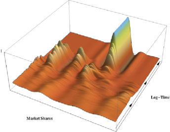
Figure 1: High sunk costs progressively transform a perfectly competitive market into an oligopoly and then into a monopoly.

In the following we illustrate how the above algorithms produce different scenarios where economic regime transitions are caused or affected by the choice of parameters, which can be structural or imposed by the policy maker during the observation period. We first consider a single market and then two interacting markets, and for simplicity we confine to the use of Algorithm 1. As a common setting to all examples we take $\mathbb{X}=[0,1]$, $n=500$, $\nu_{0}$ to be the probability distribution corresponding to a $\operatorname{Beta}(a,b)$ random variable, with $a,b>0$, with the state space discretized into 15 equally spaced intervals. The number of iterations is $5\times 10^{5}$, of which about 150 are retained at increasing distance. Every figure below shows the time evolution of the empirical measure of the market, which describes the concentration of market shares, where time is in log scale.

Figure 1 shows a single market which is in an initial state of balanced competition among firms, which have similar sizes and market shares: this can be seen by the flat side closest to the reader. As time passes, though, the high level of sunk costs, determined by setting a low $\theta$, is such that exits from the market are not compensated by the entrance of new firms, and a progressive concentration occurs. The competitive market first becomes an oligopoly, shared by no more than three or four competitors, and eventually a monopoly. Here $\nu_{0}$ corresponds to a $\operatorname{Beta}(1,1)$ and $\theta=1$. The fact that the figure shows the market attaining monopoly and staying there for a time greater than zero could be interpreted as conflicting with the diffusive nature of the process with positive (although small) entrance rate of new firms (mutation rate in population genetics terms). In this respect it is to be kept in mind, as already mentioned, that the figure is based on observations farther and farther apart in time. So the picture does not rule out the possibility of having small temporary deviations from the seeming fixation at monopoly, which, however, do not alter the long-run overall qualitative behavior.

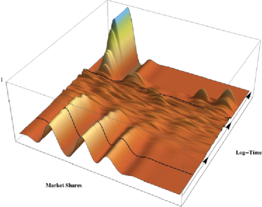
Figure 2: An Oligopoly becomes a competitive market after the policy maker reforms the sector regulation (threshold 1), and concentrates again after the reform is abolished (threshold 2).

In Figure 2 we observe a different type of transition. We initially have an oligopolistic market with three actors. The structural features of the market are such that the configuration is initially stable, until the policy maker, in correspondence to the first black solid line, introduces some new regulation which abates sunk costs or barriers to entry. Note that in the single market case the parameter $\theta$ can represent both, since this corresponds to setting $\pi=1$ in (19), while in a multiple market framework we can distinguish the two effects by means of the joint use of $\theta$ and $\pi$. Here all parameters are as in Figure 1, except $\theta$, which is set equal to 1 up to iteration 200, equal to 100 up to iteration $4.5\times 10^{4}$ and then equal to 0. The concentration level progressively decreases and the oligopoly becomes a competitive market with multiple actors. In correspondence of the second threshold, namely the second black solid line, there is a second regulation change in the opposite direction. The market concentrates again, and, from this point onward, we observe a dynamic similar to Figure 1 (recall that time is in log scale, so graphics are compressed toward the farthest side). The two thresholds can represent, for example, the effects of government alternation when opposite parties have very different political views about a certain sector.

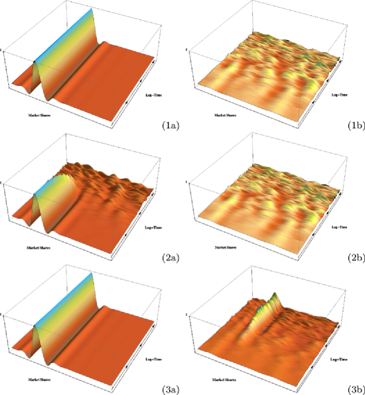
Figure 3: Effects of parameters’ change in interacting monopolistic and competitive markets. (1a) and (1b) are both closed, hence independent, markets. (2b) is closed, but (2a) has low barriers to entry ($\pi\approx 0$), and firms from (2b) progressively lower the concentration in (2a). (3b) has low barriers to entry, so that the monopolist of (3a) enters the market and conquers a dominant position.

We now proceed to illustrate some effects of the interaction between two markets with different structural properties and regulations when some of these parameters change. Figure 3 shows three scenarios regarding a monopolistic (left) and a competitive market (right). In all three cases $\nu_{0}$ corresponds to a $\operatorname{Beta}(1,1)$ for both markets. Case 1 represents independent markets, due to very high technological conversion costs or barriers to entry, which is for comparison purposes. Here $\theta_{a}=0,\theta_{b}=100$ and $\pi_{b}=1$. In Case 2 the monopolistic market has low barriers to entry, while (2b) is still closed, and a transition from monopoly to competition occurs. Here $\theta_{a}=30,\theta_{b}=100$, $\pi_{a}=0.01$, $\pi_{b}=1$. Case 3 shows the opposite setting, that is, a natural monopoly and a competitive market with low barriers to entry. The monopolist enters market (3b) and quickly assumes a dominant position. Here $\theta_{a}=0,\theta_{b}=100$, $\pi_{b}=0.7$. Recall, in this respect, the implicit effect due to setting $\beta\equiv 1$, commented upon above.

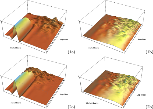
Figure 4: Firms in the competitive market (right) are polarized towards the right half of the state space. (1a) is a monopoly with high sunk costs and low barriers to entry, so firms from (1b) enters market (1a). (2a) is a monopoly with high barriers to entry and low sunk costs, so that a transition to a competitive regime occurs independently of (2b).

Case (2a) in Figure 3 suggests another point. The construction of the particle system by means of the hierarchical models defined in Section 2 compels us to have the same centering measure $\nu_{0}$, which generates new firms for all markets. In particular, this makes it essentially impossible to establish, by mere inspection of Figure 3(2a), whether the transition is due to new firms or to entrances from (2b). Relaxing this assumption on $\nu_{0}$ partially invalidates the underlying framework above, in particular, due to the fact that one loses the symmetry implied by Lemma 2.1. Nonetheless the validity of the particle system is untouched, in that the conditional distributions of type (18) are still available, where now $\nu_{0,r}$, in place of a common $\nu_{0}$, is indexed by $r\in\mathcal{I}$. This enables us to appreciate the difference between the two above mentioned effects. If one is willing to give a specific meaning to the location of the point $x\in\mathbb{X}$ which labels the firm, then $\nu_{0,r}\neq\nu_{0,r^{\prime}}$ can model the fact that, say, in two different sectors, firms are polarized on opposite sides of $\mathbb{X}$, which, in turn, represents some measurement of a certain exogenous feature possessed by those firms. Consider a monopoly and a competitive market, where we now take $\nu_{0,a}$ and $\nu_{0,b}$ to be the probability measures corresponding to a Beta($2,4$) and a Beta($4,2$) random variable for the monopolistic and competitive market, respectively. We are assuming that firms on the left half of the state space have a certain degree of difference, with respect to those on the other side, in terms of a certain characteristic. Figure 4 shows the different impact of barriers to entry and sunk costs on the monopolistic market, due to the joint use of $\pi$ and $\theta$, thus splitting Figure 3(2a) into two different scenarios. The competitive market is composed by firms which are polarized toward the right half of the state space, meaning, for example, that they have a high level of a certain feature. Then case 1 of Figure 4 shows the monopoly when sunk costs are high, but barriers to entry are low, so that the concentration is lowered by entrance of firms from the other market, rather than from the creation of new firms from within; while case 2 shows the effects of high barriers to entry and low sunk costs, so that a transition to a competitive regime occurs independently of (2b). The parameters for case 1 are $\theta_{a}=30$, $\theta_{b}=100$, $\pi_{a}=0$, $\pi_{b}=1$, while for case 2 we have $\theta_{a}=30$, $\theta_{b}=100$, $\pi_{a}=1$, $\pi_{b}=1$.

6 Concluding remarks

In this paper we propose a model for market share dynamics which is both well founded, from a theoretical point of view, and easy to implement, from a practical point of view. In illustrating its features we focus on the impact of changes in market characteristics on the behaviors of individual firms taking a macroeconomic perspective. An enrichment of the model could be achieved by incorporating exogenous information via sets of covariates. This can be done, for example, by suitably adapting the approach recently undertaken in [34] to the present framework. Alternatively, and from an economic viewpoint, more interestingly, one could modify the model adding a microeconomic understructure: this would consist of modeling explicitly the individual behavior by appropriately specifying the function $\beta_{n}$ at Point (d) in Section 3, which can account for any desired behavioral pattern of a single firm depending endogenously on both the status of all other firms and the market characteristics. This additional layer would provide a completely explicit micro-foundation of the model, allowing us to study the effect of richer types of heterogeneous individual decisions on industry and macroeconomic dynamics through comparative statics and dynamic sensitivity analysis. These issues of more economic flavor will be the focus of a forthcoming work.

Appendix A Background material

Basic elements on the Gibbs sampler

The Gibbs sampler is a special case of the Metropolis–Hastings algorithm, which, in turn, belongs to the class of Markov chain Monte Carlo procedures; see, for example, [18]. These are often applied to solve integration and optimization problems in large dimensional spaces. Suppose the integral of $f\mathchoice{\nobreak\,\colon}{\nobreak\,\colon}{\nobreak\,\colon\;}{\nobreak\,\colon\;}\mathbb{X}\rightarrow\mathbb{R}^{d}$ with respect to $\pi\in\mathscr{P}(\mathbb{X})$ is to be evaluated, and Monte Carlo integration turns out to be unfeasible. Markov chain Monte Carlo methods provide a way of constructing a stationary Markov chain with $\pi$ as the invariant measure. One can then run the chain, discard the first, say, $N$ iterations, and regard the successive output from the chain as approximate correlated samples from $\pi$, which are then used to approximate $\int f\,\mathrm{d}\pi$. The construction of a Gibbs sampler is as follows. Consider a law $\pi=\pi(\mathrm{d}x_{1},\ldots,\mathrm{d}x_{n})$ defined on $(\mathbb{X}^{n},\mathscr{X}^{n})$, and assume that the conditional distributions

$$\pi(\mathrm{d}x_{i}|x_{1},\ldots,x_{i-1},x_{i+1},\ldots,x_{n})$$

are available for every $1\leq i\leq n$. Then, given an initial set of values $(x_{1}^{0},\ldots,x_{n}^{0})$, update iteratively

$$x_{1}^{1} \sim \pi(\mathrm{d}x_{1}|x_{2}^{0},\ldots,x_{n}^{0}),$$

$$x_{2}^{1} \sim \pi(\mathrm{d}x_{2}|x_{1}^{1},x_{3}^{0},\ldots,x_{n}^{0}),$$

$$\vdots$$

$$x_{n}^{1} \sim \pi(\mathrm{d}x_{n}|x_{1}^{1},\ldots,x_{n-1}^{1}),$$

$$x_{1}^{2} \sim \pi(\mathrm{d}x_{1}|x_{2}^{1},\ldots,x_{n}^{1}),$$

and so on. Under mild conditions, this routine produces a Markov chain with equilibrium law $\pi(\mathrm{d}x_{1},\ldots,\mathrm{d}x_{n})$. The above updating rule is known as a deterministic scan. If instead the components are updated in a random order, called random scan, one also gets reversibility with respect to $\pi$.

Basic elements on Fleming–Viot processes

Fleming–Viot processes, introduced in [17], constitute, together with Dawson–Watanabe superprocesses, one of the two most studied classes of probability-measure-valued diffusions, that is, diffusion processes which take values on the space of probability measures. A review can be found in [15].

A Fleming–Viot process can be seen as a generalization of the neutral diffusion model. This describes the evolution of a vector $z=(z_{i})_{i\in S}$ representing the relative frequencies of individual types in an infinite population, where each type is identified by a point in a space $S$. The process takes values on the simplex

$$\Delta_{S}=\biggl{\{}(z_{i})_{i\in S}\in[0,1]^{S}\colon\ z_{i}\geq 0,\sum_{i\in S}z_{i}=1\biggr{\}}\\$$

and is characterized by the infinitesimal operator

$$L=\frac{1}{2}\sum_{i,j\in S}z_{i}(\delta_{ij}-z_{j})\frac{\partial^{2}}{\partial z_{i}\,\partial z_{j}}+\sum_{i\in S}b_{i}(z)\frac{\partial}{\partial z_{i}},\\$$

defined, for example, on the set $C(S)$ of continuous functions on $S$, if $S$ is compact. Here the first term drives the random genetic drift, which is the diffusive part of the process, and $b_{i}(z)$ determines the drift component, with

$$b_{i}(z)=\sum_{j\in S,j\neq i}q_{ji}z_{j}-\sum_{j\in S,j\neq i}q_{ij}z_{i}+z_{i}\biggl{(}\sum_{j\in S}\sigma_{ij}z_{j}-\sum_{k,l\in S}\sigma_{kl}z_{k}z_{l}\biggr{)},\\$$

where $q_{ij}$ is the intensity of a mutation from type $i$ to type $j$ and $\sigma_{ij}=\sigma_{ji}$ is the selection term in a diploid model. This specification is valid for $S$ finite, which yields the classical Wright–Fisher diffusion, or countably infinite; see, for example, [13]. Fleming and Viot [17] generalized to the case of an uncountable type space $S$ by characterizing the corresponding process, which takes values in the space $\mathscr{P}(S)$ of Borel probability measures on $S$, endowed with the topology of weak convergence. Its generator on functions $\phi_{m}(\mu)=F(\langle f_{1},\mu\rangle,\ldots,\langle f_{m},\mu\rangle)=F(\langle\mathbf{f},\mu\rangle)$, where $F\in C^{2}(\mathbb{R}^{m})$, $f_{1},\ldots,f_{m}$ continuous on $S$ and vanishing at infinity, for $m\geq 1$, and $\langle f,\mu\rangle=\int f\,\mathrm{d}\mu$, can be written

$$\mathbb{L}\phi(\mu) = \frac{1}{2}\sum_{i,j=1}^{m}(\langle f_{i}f_{j},\mu\rangle-\langle f_{i},\mu\rangle\langle f_{j},\mu\rangle)F_{z_{i}z_{j}}(\langle\mathbf{f},\mu\rangle)$$

$${}+\sum_{i=1}^{m}\langle Mf_{i},\mu\rangle F_{z_{i}}(\langle\mathbf{f},\mu\rangle)+\sum_{i=1}^{m}\bigl{(}\langle(f_{i}\circ\pi)\sigma,\mu^{2}\rangle-\langle f_{i},\mu\rangle\langle\sigma,\mu^{2}\rangle\bigr{)}F_{z_{i}}(\langle\mathbf{f},\mu\rangle),$$

where $\mu^{2}$ denotes product measure, $\pi$ is the projection onto the first coordinate, $M$ is the generator of a Markov process on $S$, known as the mutation operator, $\sigma$ is a non-negative, bounded, symmetric, Borel measurable functions on $S^{2}$, called selection intensity function and $F_{z_{i}}$ is the derivative of $F$ with respect to its $i$th argument. Recombination can also be included in the model.

Interacting Fleming–Viot processes

Introduced by [40], and further investigated by [7] and [6], a system of interacting Fleming–Viot processes extends a Fleming–Viot process to a collection of dependent diffusions of Fleming–Viot type, whose interaction is modeled as migration of individuals between subdivided populations. Following [6], the model without recombination can be described as follows. Let the type space be the interval $[0,1]$. Each component of the system is an element of the set $\mathscr{P}([0,1])$, denoted $\mu_{r}$ and indexed by a countable set $\mathcal{I}$ of elements $r,r^{\prime},\ldots.$ For $F\mathchoice{\nobreak\,\colon}{\nobreak\,\colon}{\nobreak\,\colon\;}{\nobreak\,\colon\;}(\mathscr{P}([0,1]))^{\mathcal{I}}\rightarrow\mathbb{R}$ of the form

$$F(\mu)=\int_{[0,1]}\cdots\int_{[0,1]}f(x_{1},\ldots,x_{m})\mu_{r_{1}}(\mathrm{d}x_{1})\cdots\mu_{r_{m}}(\mathrm{d}x_{m})$$ (38)

with $f\in C([0,1]^{m})$, $(r_{1},\ldots,r_{m})\in(\mathcal{I})^{m}$, $m\in\mathbb{N}$, the generator of a countable system of interacting Fleming–Viot processes is

$$\mathbb{G}F(\mu) = \sum_{r\in\Omega_{N}}\biggl{\{}q\int_{[0,1]}\biggl{[}\int_{[0,1]}\frac{\partial F(\mu)}{\partial\mu_{r}}(y)M^{*}(x,\mathrm{d}y)-\frac{\partial F(\mu)}{\partial\mu_{r}}(x)\biggr{]}\mu_{r}(\mathrm{d}x)$$

$$\hphantom{\sum_{r\in\Omega_{N}}\biggl{\{}}{}+c\sum_{r^{\prime}\in\Omega_{N}}a(r,r^{\prime})\int_{[0,1]}(\mu_{r^{\prime}}-\mu_{r})(\mathrm{d}x)\frac{\partial F(\mu)}{\partial\mu_{r}}(x)$$

$$\hphantom{\sum_{r\in\Omega_{N}}\biggl{\{}}{}+d\int_{[0,1]}\int_{[0,1]}\frac{\partial^{2}F(\mu)}{\partial\mu_{r}\,\partial\mu_{r}}(x,y)Q_{\mu_{r}}(\mathrm{d}x,\mathrm{d}y)$$

$$\hphantom{\sum_{r\in\Omega_{N}}\biggl{\{}}{}+s\int_{[0,1]}\int_{[0,1]}\int_{[0,1]}\frac{\partial F(\mu)}{\partial\mu_{r}}(x)\sigma(y,z)\mu_{r}(\mathrm{d}y)Q_{\mu_{r}}(\mathrm{d}x,\mathrm{d}z)\biggr{\}},$$

where the term $Q_{\mu_{r}}(\mathrm{d}x,\mathrm{d}y)=\mu_{r}(\mathrm{d}x)\delta_{x}(\mathrm{d}y)-\mu_{r}(\mathrm{d}x)\mu_{r}(\mathrm{d}y)$ drives genetic drift, $M^{*}(x,\mathrm{d}y)$ is a transition density on $[0,1]\times\mathscr{B}([0,1])$ modeling mutation, $\mathscr{B}([0,1])$ is the Borel sigma algebra on $[0,1]$, $a(\cdot,\cdot)$ on $\mathcal{I}\times\mathcal{I}$ such that $a(r,r^{\prime})\in[0,1]$ and $\sum_{r}a(r,r^{\prime})=1$ is a transition kernel modeling migration and $\sigma(\cdot,\cdot)$ is a bounded symmetric selection intensity function on $[0,1]^{2}$. The non-negative reals $q,c,d,s$ represent, respectively, the rate of mutation, immigration, resampling and selection. Let the mutation operator be

$$Mf(z)=\int[f(y)-f(z)]M^{*}(x,\mathrm{d}y),\qquad f\in B(\mathbb{X})$$ (40)

and the migration operator be

$$G^{r^{\prime}}f(z)=\int[f(y)-f(z)]\mu_{r^{\prime}}(\mathrm{d}y),\qquad f\in B(\mathbb{X}),$$ (41)

for $r^{\prime}\in\mathcal{I}$. Using this notation, and when $F$ is as in (38), (A) can be written

$$\mathbb{G}F(\mu) = \sum_{r\in\Omega_{N}}\Biggl{\{}q\sum_{i=1}^{m}\int_{[0,1]}\cdots\int_{[0,1]}M_{r_{i}}f\,\mathrm{d}\mu_{r_{1}}\cdots\,\mathrm{d}\mu_{r_{m}}$$

$$\hphantom{\sum_{r\in\Omega_{N}}\Biggl{\{}}{}+c\sum_{r^{\prime}\in\Omega_{N}}a(r,r^{\prime})\sum_{i=1}^{m}\int_{[0,1]}\cdots\int_{[0,1]}G_{r_{i}}^{r^{\prime}}f\,\mathrm{d}\mu_{r_{1}}\cdots\,\mathrm{d}\mu_{r_{m}}$$

$$\hphantom{\sum_{r\in\Omega_{N}}\Biggl{\{}}{}+d\sum_{i=1}^{m}\sum_{k\neq i}^{m}\int_{[0,1]}\cdots\int_{[0,1]}(\Phi_{r_{k,i}}f-f)\,\mathrm{d}\mu_{r_{1}}\cdots\,\mathrm{d}\mu_{r_{m}}$$

$$\hphantom{\sum_{r\in\Omega_{N}}\Biggl{\{}}{}+s\sum_{i=1}^{m}\int_{[0,1]}\cdots\int_{[0,1]}(\sigma_{r_{i},m+1}(\cdot,\cdot)f$$

$$\hphantom{\sum_{r\in\Omega_{N}}\Biggl{\{}{}+s\sum_{i=1}^{m}\int_{[0,1]}\cdots\int_{[0,1]}(}{}-\sigma_{m+1,m+2}(\cdot,\cdot)f)\,\mathrm{d}\mu_{r_{1}}\cdots\,\mathrm{d}\mu_{r_{m}}\,\mathrm{d}\mu_{r}\,\mathrm{d}\mu_{r}\Biggr{\}},$$

where $M_{j}$ and $G_{j}^{r^{\prime}}$ are $M$ and $G^{r^{\prime}}$ applied to the $j$th coordinate of $f$, $r_{i}$ is as in Proposition 4.1, $r_{k,i}$ as in (36) and $\Phi_{hj}$ as in (37). When $\mathcal{I}$ is single-valued, (A) simplifies to

$$\mathbb{G}F(\mu) = q\sum_{i=1}^{m}\langle M_{i}f,\mu^{m}\rangle+d\sum_{i=1}^{m}\sum_{k\neq i}^{m}\langle\Phi_{ki}f-f,\mu^{m}\rangle$$

$${}+s\sum_{i=1}^{m}\bigl{(}\langle\sigma_{i,m+1}(\cdot,\cdot)f,\mu^{m+1}\rangle-\langle\sigma_{m+1,m+2}(\cdot,\cdot)f,\mu^{m+2}\rangle\bigr{)},$$

which is the generator of a Fleming–Viot process with selection with $F(\mu)=\langle f,\mu^{m}\rangle$, $f\in C([0,1])$.

Appendix B Proofs

Proof of Proposition 4.1 The infinitesimal generator of the $\mathbb{X}^{n}$-valued process described at the beginning of Section 3 can be written, for any $f\in B(\mathbb{X}^{n})$, as

$$A_{n}f(\mathbf{x})=\lambda_{n}\sum_{i=1}^{n}\gamma_{n,i}\int[f(\eta_{i}(\mathbf{x}|y))-f(\mathbf{x})]q_{n,i}\bigl{(}\mathrm{d}y|\mathbf{x}_{(-i)}\bigr{)},$$ (43)

where $q_{n,i}(\mathrm{d}y|\mathbf{x}_{(-i)})$ is (4) and $\eta_{i}$ is as in (26). Within the multi-market framework, (43) is the generator of the process for the configuration of market $r$, say, conditionally on all markets $r^{\prime}\in\mathcal{I}$, $r^{\prime}\neq r$, and can be written

$$A_{D_{n}}f(\mathbf{x}^{r}|\mathcal{I}(-r))=\lambda_{n}\sum_{i=1}^{n}\gamma^{r}_{n,i}\int[f(\eta_{i}(\mathbf{x}^{r}|y))-f(\mathbf{x}^{r})]q_{{}_{D_{n},i}}(\mathrm{d}y|\mathcal{I}(-x^{r}_{i})),$$ (44)

where $\mathcal{I}(-r)$ and $\mathcal{I}(-x^{r}_{i})$ are as in (16) and (17), $\gamma_{n,i}^{r}$ are the market-specific removal probabilities and $q_{{}_{D_{n},i}}(\mathrm{d}y|\mathcal{I}(-x^{r}_{i}))$ is (18). Then the generator for the whole particle system, for every $f\in B(\mathbb{X}^{D_{n}})$, is

$$A_{D_{n}}f(\mathbf{x})=\lambda_{n}\sum_{r\in\mathcal{I}}\varrho_{r}\sum_{i=1}^{n}\gamma^{r}_{n,i}\int[f(\eta_{r_{i}}(\mathbf{x}|y))-f(\mathbf{x})]q_{{}_{D_{n},i}}(\mathrm{d}y|\mathcal{I}(-x^{r}_{i})),$$ (45)

where $\eta_{r_{i}}$ is as in (29). Setting now $\beta_{n}$ as in (24), (45) becomes

$$A_{D_{n}}f(\mathbf{x}) = \sum_{r\in\mathcal{I}}\Biggl{\{}\sum_{i=1}^{n}C_{n,r,i}\int[f(\eta_{r_{i}}(\mathbf{x}|y))-f(\mathbf{x})]\biggl{(}1+\frac{2\sigma(y)}{n}\biggr{)}\alpha_{{}_{\mathcal{I}(-r)}}(\mathrm{d}y)$$

$$\hphantom{\sum_{r\in\mathcal{I}}\Biggl{\{}}{}+\sum_{1\leq k\neq i\leq n}C_{n,r,i}[f(\eta_{r_{i}}(\mathbf{x}|x^{r}_{k}))-f(\mathbf{x})]$$

$$\hphantom{\sum_{r\in\mathcal{I}}\Biggl{\{}}{}+\frac{1}{n}\sum_{1\leq k\neq i\leq n}C_{n,r,i}\sigma(x^{r}_{k})[f(\eta_{r_{i}}(\mathbf{x}|x^{r}_{k}))-f(\mathbf{x})]\Biggr{\}},$$

with $C_{n,r,i}$ as in (25). Substituting (19) in (B) yields

$$A_{D_{n}}f(\mathbf{x}) = \sum_{r\in\mathcal{I}}\Biggl{\{}\theta\pi\sum_{i=1}^{n}C_{n,r,i}\int[f(\eta_{r_{i}}(\mathbf{x}|y))-f(\mathbf{x})]\biggl{(}1+\frac{\sigma(y)}{n}\biggr{)}\nu_{0}(\mathrm{d}y)$$

$$\hphantom{\sum_{r\in\mathcal{I}}\Biggl{\{}}{}+\theta(1-\pi)\sum_{r^{\prime}}m(r,r^{\prime})\sum_{1\leq j\neq i\leq n}C_{n,r,i}\int[f(\eta_{r_{i}}(\mathbf{x}|y))-f(\mathbf{x})]$$

$$\hphantom{\sum_{r\in\mathcal{I}}\Biggl{\{}{}+\;}{}\times\biggl{(}1+\frac{\sigma(y)}{n}\biggr{)}\mu_{r^{\prime}}(\mathrm{d}y)$$

$$\hphantom{\sum_{r\in\mathcal{I}}\Biggl{\{}}{}+\sum_{1\leq k\neq i\leq n}C_{n,r,i}[f(\eta_{r_{i}}(\mathbf{x}|x^{r}_{k}))-f(\mathbf{x})]$$

$$\hphantom{\sum_{r\in\mathcal{I}}\Biggl{\{}}{}+\frac{1}{n}\sum_{1\leq k\neq i\leq n}C_{n,r,i}\sigma(x^{r}_{k})[f(\eta_{r_{i}}(\mathbf{x}|x^{r}_{k}))-f(\mathbf{x})]\Biggr{\}}.$$

By means of (27) and (28), with $M_{i}^{n}f$ and $G_{i}^{n,r^{\prime}}f$ denoting, respectively, $M^{n}$ and $G^{n,r^{\prime}}$, applied to the $i$th coordinate of $f$, and $M_{r_{i}}^{n}f$ and $G_{r_{i}}^{n,r^{\prime}}f$ interpreted according to (29), (B) can be written

$$A_{D_{n}}f(\mathbf{x}) = \sum_{r\in\mathcal{I}}\Biggl{\{}\theta\pi\sum_{i=1}^{n}C_{n,r,i}M_{r_{i}}^{n}f(\mathbf{x})$$

$$\hphantom{\sum_{r\in\mathcal{I}}\Biggl{\{}}{}+\theta(1-\pi)\sum_{r^{\prime}}m(r,r^{\prime})\sum_{i=1}^{n}C_{n,r,i}G_{r_{i}}^{n,r^{\prime}}f(\mathbf{x})$$

$$\hphantom{\sum_{r\in\mathcal{I}}\Biggl{\{}}{}+\sum_{1\leq k\neq i\leq n}C_{n,r,i}[f(\eta_{r_{i}}(\mathbf{x}|x^{r}_{k}))-f(\mathbf{x})]$$

$$\hphantom{\sum_{r\in\mathcal{I}}\Biggl{\{}}{}+\frac{1}{n}\sum_{1\leq k\neq i\leq n}C_{n,r,i}\sigma(x^{r}_{k})[f(\eta_{r_{i}}(\mathbf{x}|x^{r}_{k}))-f(\mathbf{x})]\Biggr{\}}.$$

Proof of Proposition 4.2 For $k\leq n$, let $n_{[k]}$ be as in (32), and define the probability measure

$$\mu^{(D_{k})}=\prod_{r\in\mathcal{I}}\frac{1}{n_{[k]}}\sum_{1\leq i_{r,1}\neq\cdots\neq i_{r,k}\leq n}\delta_{(x^{r}_{i_{r,1}},\ldots,x^{r}_{i_{r,k}})},$$ (48)

where $D_{k}$ is as in (14). Define also

$$\phi_{D_{k}}(\mu)=\bigl{\langle}f,\mu^{(D_{k})}\bigr{\rangle},\qquad f\in B(\mathbb{X}^{D_{k}})$$

and

$$\mathbb{A}_{D_{n}}\phi_{D_{k}}(\mu)=\bigl{\langle}A_{D_{n}}f,\mu^{(D_{k})}\bigr{\rangle},$$ (49)

where $\langle f,\mu\rangle=\int f\,\mathrm{d}\mu$. Then $\mathbb{A}_{D_{n}}\phi_{D_{n}}(\mu)$ is the generator of the $(\mathscr{P}(\mathbb{X}))^{\#\mathcal{I}}$-valued system (31), which from (4.1), letting $f\in B(\mathbb{X}^{D_{n}})$ in (49), can be written

$$\mathbb{A}_{D_{n}}\phi_{D_{n}}(\mu) = \sum_{r\in\mathcal{I}}\Biggl{[}\theta\pi\sum_{i=1}^{n}C_{n,r,i}\langle M_{r_{i}}^{n}f,\mu^{(D_{n})}\rangle$$

$$\hphantom{\sum_{r\in\mathcal{I}}\Biggl{[}}{}+\theta(1-\pi)\sum_{r^{\prime}}m(r,r^{\prime})\sum_{i=1}^{n}C_{n,r,i}\bigl{\langle}G_{r_{i}}^{n,r^{\prime}}f,\mu^{(D_{n})}\bigr{\rangle}$$

$$\hphantom{\sum_{r\in\mathcal{I}}\Biggl{[}}{}+\sum_{1\leq k\neq i\leq n}C_{n,r,i}\bigl{\langle}\Phi_{r_{k,i}}f-f,\mu^{(D_{n})}\bigr{\rangle}$$

$$\hphantom{\sum_{r\in\mathcal{I}}\Biggl{[}}{}+\frac{1}{n}\sum_{1\leq k\neq i\leq n}C_{n,r,i}\bigl{\langle}\sigma_{r_{k}}(\cdot)(\Phi_{r_{k,i}}f-f),\mu^{(D_{n})}\bigr{\rangle}\Biggr{]},$$

where $\sigma_{r_{k}}(\cdot)$ denotes $\sigma(x^{r}_{k})$ and $\Phi_{ki}$ is as in (37). Note now that for $f\in B(\mathbb{X}^{m})$, $m\leq D_{n}$, we have

$$M_{r_{i}}^{n}f=f,\qquad G_{r_{i}}^{n,r^{\prime}}f=f,\qquad\Phi_{r_{k,i}}f=f,\qquad\mbox{if }i>m$$

and

$$\bigl{\langle}\Phi_{r_{k,i}}f,\mu^{(m)}\bigr{\rangle}=\bigl{\langle}f,\mu^{(m)}\bigr{\rangle},\qquad i\leq m,m+1\leq k\leq n.$$

Given (33) and (34), it follows that when $f\in B(\mathbb{X}^{m})$, $m\leq D_{n}$, (B) can be written

$$\mathbb{A}_{D_{n}}\phi_{m}(\mu) = \sum_{r\in\mathcal{I}}\Biggl{\{}\theta\pi\sum_{i=1}^{m}C_{n,r,i}\bigl{\langle}M_{r_{i}}^{n}f,\mu^{(m)}\bigr{\rangle}$$

$$\hphantom{\sum_{r\in\mathcal{I}}\Biggl{\{}}{}+\theta(1-\pi)\sum_{r^{\prime}}a(r,r^{\prime})\sum_{i=1}^{m}C_{n,r,i}\bigl{\langle}G_{r_{i}}^{n,r^{\prime}}f,\mu^{(m)}\bigr{\rangle}$$

$$\hphantom{\sum_{r\in\mathcal{I}}\Biggl{\{}}{}+\sum_{1\leq k\neq i\leq m}C_{n,r,i}\bigl{\langle}\Phi_{r_{k,i}}f-f,\mu^{(m)}\bigr{\rangle}$$

$$\hphantom{\sum_{r\in\mathcal{I}}\Biggl{\{}}{}+\frac{1}{n}\sum_{i=1}^{m}\sum_{k\neq i}^{k_{r}}C_{n,r,i}\bigl{\langle}\sigma_{r_{k}}(\cdot)(\Phi_{r_{k,i}}f-f),\mu^{(m)}\bigr{\rangle}$$

$$\hphantom{\sum_{r\in\mathcal{I}}\Biggl{\{}}{}+\frac{n-k_{r}}{n}\sum_{i=1}^{m}C_{n,r,i}\bigl{\langle}\sigma_{m+1}(\cdot)(\Phi_{m+1,r_{i}}f-f),\mu^{(m)}\mu_{r}\bigr{\rangle}\Biggr{\}}.$$

Proof of Theorem 4.3For $f\in B(\mathbb{X}^{k})$, $k\geq 1$, let $\|f\|=\sup_{x\in\mathbb{X}^{k}}|f(x)|$. Observe that (27) and (28) converge uniformly, respectively to (40) and (41), as $n$ tends to infinity, implying

$$\bigl{\|}\bigl{\langle}M^{n}_{r_{i}}f,\mu^{(m)}\bigr{\rangle}-\bigl{\langle}M_{r_{i}}f,\mu^{(m)}\bigr{\rangle}\bigr{\|} \rightarrow 0 ,\qquad f\in B(\mathbb{X}^{m}),$$

$$\bigl{\|}\bigl{\langle}G^{n,r^{\prime}}_{r_{i}}f,\mu^{(m)}\bigr{\rangle}-\bigl{\langle}G^{r^{\prime}}_{r_{i}}f,\mu^{(m)}\bigr{\rangle}\bigr{\|} \rightarrow 0 ,\qquad f\in B(\mathbb{X}^{m}).$$

Here the supremum norm is intended with respect to the vector $x\in\mathbb{X}^{m}$ of atoms in $\mu^{(m)}$, with $\mu^{(m)}$ as in (34). Let now $\mu^{(k_{r})}_{r}$ be as in (33), so that $\mu_{r}=n^{-1}\sum_{i=1}^{n}\delta_{x^{r}_{i}}$. Then it is easy to check that

$$\bigl{\|}\bigl{\langle}f,\mu^{(k_{r})}_{r}\bigr{\rangle}-\bigl{\langle}f,\mu_{r}^{k_{r}}\bigr{\rangle}\bigr{\|}\rightarrow 0,\qquad f\in B(\mathbb{X}^{k_{r}}),$$

as $n\rightarrow\infty$, where $\mu^{k_{r}}$ denotes a $k_{r}$-fold product measure $\mu_{r}\times\cdots\times\mu_{r}$, and that

$$\bigl{\|}\bigl{\langle}f,\mu^{(m)}\bigr{\rangle}-\langle f,\mu^{\times m}\rangle\bigr{\|}\rightarrow 0,\qquad f\in B(\mathbb{X}^{m}),$$

as $n\rightarrow\infty$, where we have denoted

$$\mu^{\times m}=\prod_{r\in\mathcal{I}}\mu_{r}^{k_{r}}.$$

We also have, from (25) $C_{n,r,i}=\lambda_{n}\varrho_{r}\gamma_{n,i}^{r}/\bar{q}_{{}_{D_{n},i}}$, where $\lambda_{n}$ is the Poisson rate driving the holding times, $\varrho_{r}=\mathrm{O}(\#\mathcal{I}^{-1})$ and $\gamma^{r}_{n,i}=\mathrm{O}(n^{-1})$ are the probability of choosing market $r$ and $x^{r}_{i}$ respectively during the update, and $\bar{q}_{{}_{D_{n},i}}=\mathrm{O}(n)$ is the normalizing constant of (3). Then choosing $\lambda_{n}=\mathrm{O}(nD_{n})=\mathrm{O}(n^{2}\#\mathcal{I})$ implies $C_{n,r,i}\rightarrow 1$ as $n\rightarrow\infty$. Finally, let $\varphi_{m}\in B(\mathscr{P}(\mathbb{X}^{m}))$ be

$$\varphi_{m}(\mu)=\langle f,\mu^{\times m}\rangle=\int_{[0,1]}\cdots\int_{[0,1]}f(x_{1},\ldots,x_{m})\mu_{r_{1}}(\mathrm{d}x_{1})\cdots\mu_{r_{m}}(\mathrm{d}x_{m})$$ (51)

for any sequence $(r_{1},\ldots,r_{m})\in\mathcal{I}^{m}$. Then it can be checked that (4.2) converges, as $n$ tends to infinity, to

$$\mathbb{A}\varphi_{m}(\mu) = \sum_{r\in\mathcal{I}}\Biggl{[}\theta\pi\sum_{i=1}^{m}\langle M_{r_{i}}f,\mu^{\times m}\rangle+\theta(1-\pi)\sum_{r^{\prime}\in\mathcal{I}}m(r,r^{\prime})\sum_{i=1}^{m}\langle G_{r_{i}}^{r^{\prime}}f,\mu^{\times m}\rangle$$

$$\hphantom{\sum_{r\in\mathcal{I}}\Biggl{[}}{}+\sum_{1\leq k\neq i\leq m}\langle\Phi_{r_{k,i}}f-f,\mu^{\times m}\rangle+\sum_{i=1}^{m}\langle\sigma_{r_{i}}(\cdot)f-\sigma_{m+1}(\cdot)f,\mu^{\times m}\mu_{r}\rangle\Biggr{]}$$

which, in turn, implies

$$\|\mathbb{A}_{D_{n}}\phi_{m}(\mu)-\mathbb{A}\varphi_{m}(\mu)\|\longrightarrow 0\qquad\mbox{as }n\rightarrow\infty.$$

Using (51), and letting $\mathbb{X}=[0,1]$, $\mathbb{A}\varphi_{m}(\mu)$ can be written

$$\mathbb{A}\varphi_{m}(\mu) = \sum_{r\in\mathcal{I}}\Biggl{[}\theta\pi\sum_{i=1}^{m}\int_{[0,1]}\cdots\int_{[0,1]}M_{r_{i}}f\,\mathrm{d}\mu_{r_{1}}\cdots\,\mathrm{d}\mu_{r_{m}}$$

$$\hphantom{\sum_{r\in\mathcal{I}}\Biggl{[}}{}+\theta(1-\pi)\sum_{r^{\prime}\in\mathcal{I}}m(r,r^{\prime})\sum_{i=1}^{m}\int_{[0,1]}\cdots\int_{[0,1]}G_{r_{i}}^{r^{\prime}}f\,\mathrm{d}\mu_{r_{1}}\cdots\,\mathrm{d}\mu_{r_{m}}$$

$$\hphantom{\sum_{r\in\mathcal{I}}\Biggl{[}}{}+\sum_{1\leq k\neq i\leq m}\int_{[0,1]}\cdots\int_{[0,1]}(\Phi_{r_{k,i}}f-f)\,\mathrm{d}\mu_{r_{1}}\cdots\,\mathrm{d}\mu_{r_{m}}$$

$$\hphantom{\sum_{r\in\mathcal{I}}\Biggl{[}}{}+\sum_{i=1}^{m}\int_{[0,1]}\cdots\int_{[0,1]}\bigl{(}\sigma_{r_{i}}(\cdot)f-\sigma_{m+1}(\cdot)f\bigr{)}\,\mathrm{d}\mu_{r_{1}}\cdots\,\mathrm{d}\mu_{r_{m}}\,\mathrm{d}\mu_{r}\Biggr{]},$$

which equals (A) for appropriate values of $q,c,d,s$ and for univariate $\sigma$. The statement with $C_{\mathscr{P}(\mathbb{X})^{\#\mathcal{I}}}([0,\infty))$ replaced by $D_{\mathscr{P}(\mathbb{X})^{\#\mathcal{I}}}([0,\infty))$ now follows from Theorems 1.6.1 and 4.2.11 of [14], which, respectively, imply the strong convergence of the corresponding semigroups and the weak convergence of the law of $Y^{(n)}(\cdot)$ to that of $Y(\cdot)$. Replacing $D_{\mathscr{P}(\mathbb{X})^{\#\mathcal{I}}}([0,\infty))$ with $C_{\mathscr{P}(\mathbb{X})^{\#\mathcal{I}}}([0,\infty))$ follows from [1], Section 18, by relativization of the Skorohod topology to $C_{\mathscr{P}(\mathbb{X})^{\#\mathcal{I}}}([0,\infty))$.

References

- [1] {bbook}[mr] \bauthor\bsnmBillingsley, \bfnmPatrick\binitsP. (\byear1968). \btitleConvergence of Probability Measures. \baddressNew York: \bpublisherWiley. \bidmr=0233396 \bptokimsref \endbibitem
- [2] {barticle}[mr] \bauthor\bsnmBlackwell, \bfnmDavid\binitsD. &\bauthor\bsnmMacQueen, \bfnmJames B.\binitsJ.B. (\byear1973). \btitleFerguson distributions via Pólya urn schemes. \bjournalAnn. Statist. \bvolume1 \bpages353–355. \bidissn=0090-5364, mr=0362614 \bptokimsref \endbibitem
- [3] {barticle}[mr] \bauthor\bsnmBurda, \bfnmMartin\binitsM., \bauthor\bsnmHarding, \bfnmMatthew\binitsM. &\bauthor\bsnmHausman, \bfnmJerry\binitsJ. (\byear2008). \btitleA Bayesian mixed logit-probit model for multinomial choice. \bjournalJ. Econometrics \bvolume147 \bpages232–246. \biddoi=10.1016/j.jeconom.2008.09.029, issn=0304-4076, mr=2478523 \bptokimsref \endbibitem
- [4] {barticle}[mr] \bauthor\bsnmCifarelli, \bfnmDonato Michele\binitsD.M. &\bauthor\bsnmRegazzini, \bfnmEugenio\binitsE. (\byear1996). \btitleDe Finetti’s contribution to probability and statistics. \bjournalStatist. Sci. \bvolume11 \bpages253–282. \biddoi=10.1214/ss/1032280303, issn=0883-4237, mr=1445983 \bptokimsref \endbibitem
- [5] {barticle}[mr] \bauthor\bsnmDai Pra, \bfnmPaolo\binitsP., \bauthor\bsnmRunggaldier, \bfnmWolfgang J.\binitsW.J., \bauthor\bsnmSartori, \bfnmElena\binitsE. &\bauthor\bsnmTolotti, \bfnmMarco\binitsM. (\byear2009). \btitleLarge portfolio losses: A dynamic contagion model. \bjournalAnn. Appl. Probab. \bvolume19 \bpages347–394. \biddoi=10.1214/08-AAP544, issn=1050-5164, mr=2498681 \bptokimsref \endbibitem
- [6] {barticle}[mr] \bauthor\bsnmDawson, \bfnmDonald A.\binitsD.A. &\bauthor\bsnmGreven, \bfnmAndreas\binitsA. (\byear1999). \btitleHierarchically interacting Fleming–Viot processes with selection and mutation: Multiple space time scale analysis and quasi-equilibria. \bjournalElectron. J. Probab. \bvolume4 \bpagesno. 4, 81 pp. (electronic). \bidissn=1083-6489, mr=1670873 \bptokimsref \endbibitem
- [7] {barticle}[mr] \bauthor\bsnmDawson, \bfnmDonald A.\binitsD.A., \bauthor\bsnmGreven, \bfnmAndreas\binitsA. &\bauthor\bsnmVaillancourt, \bfnmJean\binitsJ. (\byear1995). \btitleEquilibria and quasiequilibria for infinite collections of interacting Fleming–Viot processes. \bjournalTrans. Amer. Math. Soc. \bvolume347 \bpages2277–2360. \biddoi=10.2307/2154827, issn=0002-9947, mr=1297523 \bptokimsref \endbibitem
- [8] {barticle}[mr] \bauthor\bsnmDe Blasi, \bfnmPierpaolo\binitsP., \bauthor\bsnmJames, \bfnmLancelot F.\binitsL.F. &\bauthor\bsnmLau, \bfnmJohn W.\binitsJ.W. (\byear2010). \btitleBayesian nonparametric estimation and consistency of mixed multinomial logit choice models. \bjournalBernoulli \bvolume16 \bpages679–704. \biddoi=10.3150/09-BEJ233, issn=1350-7265, mr=2730644 \bptokimsref \endbibitem
- [9] {barticle}[mr] \bauthor\bsnmDe Iorio, \bfnmMaria\binitsM., \bauthor\bsnmMüller, \bfnmPeter\binitsP., \bauthor\bsnmRosner, \bfnmGary L.\binitsG.L. &\bauthor\bsnmMacEachern, \bfnmSteven N.\binitsS.N. (\byear2004). \btitleAn ANOVA model for dependent random measures. \bjournalJ. Amer. Statist. Assoc. \bvolume99 \bpages205–215. \biddoi=10.1198/016214504000000205, issn=0162-1459, mr=2054299 \bptokimsref \endbibitem
- [10] {barticle}[mr] \bauthor\bsnmDuan, \bfnmJason A.\binitsJ.A., \bauthor\bsnmGuindani, \bfnmMichele\binitsM. &\bauthor\bsnmGelfand, \bfnmAlan E.\binitsA.E. (\byear2007). \btitleGeneralized spatial Dirichlet process models. \bjournalBiometrika \bvolume94 \bpages809–825. \biddoi=10.1093/biomet/asm071, issn=0006-3444, mr=2416794 \bptokimsref \endbibitem
- [11] {barticle}[mr] \bauthor\bsnmDunson, \bfnmDavid B.\binitsD.B. &\bauthor\bsnmPark, \bfnmJu-Hyun\binitsJ.H. (\byear2008). \btitleKernel stick-breaking processes. \bjournalBiometrika \bvolume95 \bpages307–323. \biddoi=10.1093/biomet/asn012, issn=0006-3444, mr=2521586 \bptokimsref \endbibitem
- [12] {barticle}[auto:STB—2011/12/15—13:36:40] \bauthor\bsnmEricson, \bfnmR.\binitsR. &\bauthor\bsnmPakes, \bfnmA.\binitsA. (\byear1985). \btitleMarkov-perfect industry dynamics: A framework for empirical work. \bjournalRev. Econ. Stud. \bvolume62 \bpages53–82. \bptokimsref \endbibitem
- [13] {barticle}[mr] \bauthor\bsnmEthier, \bfnmS. N.\binitsS.N. (\byear1981). \btitleA class of infinite-dimensional diffusions occurring in population genetics. \bjournalIndiana Univ. Math. J. \bvolume30 \bpages925–935. \biddoi=10.1512/iumj.1981.30.30068, issn=0022-2518, mr=0632861 \bptokimsref \endbibitem
- [14] {bbook}[mr] \bauthor\bsnmEthier, \bfnmStewart N.\binitsS.N. &\bauthor\bsnmKurtz, \bfnmThomas G.\binitsT.G. (\byear1986). \btitleMarkov Processes: Characterization and Convergence. \bseriesWiley Series in Probability and Mathematical Statistics. \baddressNew York: \bpublisherWiley. \biddoi=10.1002/9780470316658, mr=0838085 \bptokimsref \endbibitem
- [15] {barticle}[mr] \bauthor\bsnmEthier, \bfnmS. N.\binitsS.N. &\bauthor\bsnmKurtz, \bfnmThomas G.\binitsT.G. (\byear1993). \btitleFleming–Viot processes in population genetics. \bjournalSIAM J. Control Optim. \bvolume31 \bpages345–386. \biddoi=10.1137/0331019, issn=0363-0129, mr=1205982 \bptokimsref \endbibitem
- [16] {barticle}[mr] \bauthor\bsnmFerguson, \bfnmThomas S.\binitsT.S. (\byear1973). \btitleA Bayesian analysis of some nonparametric problems. \bjournalAnn. Statist. \bvolume1 \bpages209–230. \bidissn=0090-5364, mr=0350949 \bptokimsref \endbibitem
- [17] {barticle}[mr] \bauthor\bsnmFleming, \bfnmWendell H.\binitsW.H. &\bauthor\bsnmViot, \bfnmMichel\binitsM. (\byear1979). \btitleSome measure-valued Markov processes in population genetics theory. \bjournalIndiana Univ. Math. J. \bvolume28 \bpages817–843. \biddoi=10.1512/iumj.1979.28.28058, issn=0022-2518, mr=0542340 \bptokimsref \endbibitem
- [18] {barticle}[mr] \bauthor\bsnmGelfand, \bfnmAlan E.\binitsA.E. &\bauthor\bsnmSmith, \bfnmAdrian F. M.\binitsA.F.M. (\byear1990). \btitleSampling-based approaches to calculating marginal densities. \bjournalJ. Amer. Statist. Assoc. \bvolume85 \bpages398–409. \bidissn=0162-1459, mr=1141740 \bptokimsref \endbibitem
- [19] {barticle}[auto:STB—2011/12/15—13:36:40] \bauthor\bsnmGriffin, \bfnmJ. E.\binitsJ.E. (\byear2011). \btitleThe Ornstein–Uhlenbeck Dirichlet process and other time-varying processes for Bayesian nonparametric inference. \bjournalJ. Statist. Plann. Inference \bvolume141 \bpages3648–3664. \bptokimsref \endbibitem
- [20] {barticle}[mr] \bauthor\bsnmGriffin, \bfnmJ. E.\binitsJ.E. &\bauthor\bsnmSteel, \bfnmM. F. J.\binitsM.F.J. (\byear2004). \btitleSemiparametric Bayesian inference for stochastic frontier models. \bjournalJ. Econometrics \bvolume123 \bpages121–152. \biddoi=10.1016/j.jeconom.2003.11.001, issn=0304-4076, mr=2126161 \bptokimsref \endbibitem
- [21] {barticle}[mr] \bauthor\bsnmGriffin, \bfnmJ. E.\binitsJ.E. &\bauthor\bsnmSteel, \bfnmM. F. J.\binitsM.F.J. (\byear2006). \btitleOrder-based dependent Dirichlet processes. \bjournalJ. Amer. Statist. Assoc. \bvolume101 \bpages179–194. \biddoi=10.1198/016214505000000727, issn=0162-1459, mr=2268037 \bptokimsref \endbibitem
- [22] {barticle}[mr] \bauthor\bsnmGriffin, \bfnmJ. E.\binitsJ.E. &\bauthor\bsnmSteel, \bfnmM. F. J.\binitsM.F.J. (\byear2011). \btitleStick-breaking autoregressive processes. \bjournalJ. Econometrics \bvolume162 \bpages383–396. \biddoi=10.1016/j.jeconom.2011.03.001, issn=0304-4076, mr=2795625 \bptokimsref \endbibitem
- [23] {bbook}[mr] \bauthor\bsnmHjort, \bfnmN. L.\binitsN.L., \bauthor\bsnmHolmes, \bfnmC. C.\binitsC.C., \bauthor\bsnmMüller, \bfnmP.\binitsP. &\bauthor\bsnmWalker, \bfnmS. G.\binitsS.G., eds. (\byear2010). \btitleBayesian Nonparametrics. \bseriesCambridge Series in Statistical and Probabilistic Mathematics. \baddressCambridge: \bpublisherCambridge Univ. Press. \bidmr=2722987 \bptokimsref \endbibitem
- [24] {barticle}[mr] \bauthor\bsnmHopenhayn, \bfnmHugo A.\binitsH.A. (\byear1992). \btitleEntry, exit, and firm dynamics in long run equilibrium. \bjournalEconometrica \bvolume60 \bpages1127–1150. \biddoi=10.2307/2951541, issn=0012-9682, mr=1180236 \bptokimsref \endbibitem
- [25] {barticle}[mr] \bauthor\bsnmIshwaran, \bfnmHemant\binitsH. &\bauthor\bsnmJames, \bfnmLancelot F.\binitsL.F. (\byear2001). \btitleGibbs sampling methods for stick-breaking priors. \bjournalJ. Amer. Statist. Assoc. \bvolume96 \bpages161–173. \biddoi=10.1198/016214501750332758, issn=0162-1459, mr=1952729 \bptokimsref \endbibitem
- [26] {barticle}[mr] \bauthor\bsnmJovanovic, \bfnmBoyan\binitsB. (\byear1982). \btitleSelection and the evolution of industry. \bjournalEconometrica \bvolume50 \bpages649–670. \biddoi=10.2307/1912606, issn=0012-9682, mr=0662724 \bptokimsref \endbibitem
- [27] {barticle}[mr] \bauthor\bsnmLau, \bfnmJohn W.\binitsJ.W. &\bauthor\bsnmSiu, \bfnmTak Kuen\binitsT.K. (\byear2008). \btitleModelling long-term investment returns via Bayesian infinite mixture time series models. \bjournalScand. Actuar. J. \bvolume4 \bpages243–282. \biddoi=10.1080/03461230701862889, issn=0346-1238, mr=2484128 \bptokimsref \endbibitem
- [28] {barticle}[mr] \bauthor\bsnmLau, \bfnmJohn W.\binitsJ.W. &\bauthor\bsnmSiu, \bfnmTak Kuen\binitsT.K. (\byear2008). \btitleOn option pricing under a completely random measure via a generalized Esscher transform. \bjournalInsurance Math. Econom. \bvolume43 \bpages99–107. \biddoi=10.1016/j.insmatheco.2008.03.006, issn=0167-6687, mr=2442035 \bptokimsref \endbibitem
- [29] {barticle}[mr] \bauthor\bsnmLo, \bfnmAlbert Y.\binitsA.Y. (\byear1984). \btitleOn a class of Bayesian nonparametric estimates. I. Density estimates. \bjournalAnn. Statist. \bvolume12 \bpages351–357. \biddoi=10.1214/aos/1176346412, issn=0090-5364, mr=0733519 \bptokimsref \endbibitem
- [30] {bincollection}[auto:STB—2011/12/15—13:36:40] \bauthor\bsnmMacEachern, \bfnmS. N.\binitsS.N. (\byear1999). \btitleDependent nonparametric Processes. In \bbooktitleASA Proc. of the Section on Bayesian Statistical Science. \baddressAlexandria, VA: \bpublisherAmer. Statist. Assoc. \bptokimsref \endbibitem
- [31] {bmisc}[auto:STB—2011/12/15—13:36:40] \bauthor\bsnmMacEachern, \bfnmS. N.\binitsS.N. (\byear2000). \bhowpublishedDependent Dirichlet processes. Technical Report, Ohio State Univ. \bptokimsref \endbibitem
- [32] {bmisc}[auto:STB—2011/12/15—13:36:40] \bauthor\bsnmMartin, \bfnmA.\binitsA., \bauthor\bsnmPrünster, \bfnmI.\binitsI., \bauthor\bsnmRuggiero, \bfnmM.\binitsM. &\bauthor\bsnmTaddei, \bfnmF.\binitsF. (\byear2012). \bhowpublishedInefficient credit cycles via generalized Pólya urn schemes. Working paper. \bptokimsref \endbibitem
- [33] {barticle}[mr] \bauthor\bsnmMena, \bfnmRamsés H.\binitsR.H. &\bauthor\bsnmWalker, \bfnmStephen G.\binitsS.G. (\byear2005). \btitleStationary autoregressive models via a Bayesian nonparametric approach. \bjournalJ. Time Ser. Anal. \bvolume26 \bpages789–805. \biddoi=10.1111/j.1467-9892.2005.00429.x, issn=0143-9782, mr=2203511 \bptokimsref \endbibitem
- [34] {barticle}[mr] \bauthor\bsnmPark, \bfnmJu-Hyun\binitsJ.H. &\bauthor\bsnmDunson, \bfnmDavid B.\binitsD.B. (\byear2010). \btitleBayesian generalized product partition model. \bjournalStatist. Sinica \bvolume20 \bpages1203–1226. \bidissn=1017-0405, mr=2730180 \bptokimsref \endbibitem
- [35] {barticle}[mr] \bauthor\bsnmPetrone, \bfnmSonia\binitsS., \bauthor\bsnmGuindani, \bfnmMichele\binitsM. &\bauthor\bsnmGelfand, \bfnmAlan E.\binitsA.E. (\byear2009). \btitleHybrid Dirichlet mixture models for functional data. \bjournalJ. R. Stat. Soc. Ser. B Stat. Methodol. \bvolume71 \bpages755–782. \biddoi=10.1111/j.1467-9868.2009.00708.x, issn=1369-7412, mr=2750094 \bptokimsref \endbibitem
- [36] {barticle}[mr] \bauthor\bsnmRemenik, \bfnmDaniel\binitsD. (\byear2009). \btitleLimit theorems for individual-based models in economics and finance. \bjournalStochastic Process. Appl. \bvolume119 \bpages2401–2435. \biddoi=10.1016/j.spa.2008.12.001, issn=0304-4149, mr=2532206 \bptokimsref \endbibitem
- [37] {barticle}[mr] \bauthor\bsnmRuggiero, \bfnmMatteo\binitsM. &\bauthor\bsnmWalker, \bfnmStephen G.\binitsS.G. (\byear2009). \btitleBayesian nonparametric construction of the Fleming–Viot process with fertility selection. \bjournalStatist. Sinica \bvolume19 \bpages707–720. \bidissn=1017-0405, mr=2514183 \bptokimsref \endbibitem
- [38] {barticle}[auto:STB—2011/12/15—13:36:40] \bauthor\bsnmSutton, \bfnmJ.\binitsJ. (\byear2007). \btitleMarket share dynamics and the “persistence of leadership” debate. \bjournalAmer. Econ. Rev. \bvolume97 \bpages222–241. \bptokimsref \endbibitem
- [39] {barticle}[auto:STB—2011/12/15—13:36:40] \bauthor\bsnmTrippa, \bfnmL.\binitsL., \bauthor\bsnmMüller, \bfnmP.\binitsP. &\bauthor\bsnmJohnson, \bfnmW.\binitsW. (\byear2011). \btitleThe multivariate beta process and an extension of the Pólya tree model. \bjournalBiometrika \bvolume98 \bpages17–34. \bptokimsref \endbibitem
- [40] {barticle}[mr] \bauthor\bsnmVaillancourt, \bfnmJean\binitsJ. (\byear1990). \btitleInteracting Fleming–Viot processes. \bjournalStochastic Process. Appl. \bvolume36 \bpages45–57. \biddoi=10.1016/0304-4149(90)90041-P, issn=0304-4149, mr=1075600 \bptokimsref \endbibitem
- [41] {barticle}[mr] \bauthor\bsnmWalker, \bfnmStephen\binitsS. &\bauthor\bsnmMuliere, \bfnmPietro\binitsP. (\byear2003). \btitleA bivariate Dirichlet process. \bjournalStatist. Probab. Lett. \bvolume64 \bpages1–7. \biddoi=10.1016/S0167-7152(03)00124-X, issn=0167-7152, mr=1995803 \bptokimsref \endbibitem