An extended family of circular distributions related to wrapped Cauchy distributions via Brownian motion

Abstract

We introduce a four-parameter extended family of distributions related to the wrapped Cauchy distribution on the circle. The proposed family can be derived by altering the settings of a problem in Brownian motion which generates the wrapped Cauchy. The densities of this family have a closed form and can be symmetric or asymmetric depending on the choice of the parameters. Trigonometric moments are available, and they are shown to have a simple form. Further tractable properties of the model are obtained, many by utilizing the trigonometric moments. Other topics related to the model, including alternative derivations and Möbius transformation, are considered. Discussion of the symmetric submodels is given. Finally, generalization to a family of distributions on the sphere is briefly made.

and

1 Introduction

As a unimodal and symmetric model on the circle, the wrapped Cauchy or circular Cauchy distribution has played an important role in directional statistics. It has density

$$f(\theta;\mu,\rho)=\frac{1}{2\uppi}\frac{1-\rho^{2}}{1+\rho^{2}-2\rho\cos(\theta-\mu)},\qquad-\uppi\leq\theta<\uppi,$$ (1)

where $\mu\ (\in[-\uppi,\uppi))$ is a location parameter, and $\rho\ (\in[0,1))$ controls the concentration of the model. This distribution has some desirable mathematical features, as discussed in Kent and Tyler [11] and McCullagh [15]. We write $\Theta\sim\operatorname{WC}(\mu,\rho)$ if a random variable $\Theta$ has density (1).

In modeling symmetric circular data, the wrapped Cauchy distribution could be one choice as well as other familiar symmetric models such as the von Mises and wrapped normal distributions; see also Jones and Pewsey [7]. In reality, however, it is not so common to find such data in fields of application. In many cases the data of interest are asymmetrically distributed, and therefore probability distributions having asymmetric densities are desired.

Construction of a tractable circular model with an asymmetric shape has been a problem in statistics of circular data. To tackle this problem, some asymmetric extensions of well-known circular models have been proposed in the literature. Maksimov [12], Yfantis and Borgman [20] and Gatto and Jammalamadaka [4] discussed an extension of the von Mises distribution, generated through maximization of Shannon’s entropy with restrictions on certain trigonometric moments. Batschelet [2] proposed a mathematical method of skewing circular distributions that has seen renewed interest very recently. Pewsey [16] presented a four-parameter family of distributions on the circle by wrapping the stable distribution, which is asymmetric, onto the circle. Recent work by Kato and Jones [9] proposed a family of distributions arising from the Möbius transformation which includes the von Mises and wrapped Cauchy distributions. Unlike familiar symmetric distributions, it is often difficult to deal with skew models in statistical analysis. This difficulty is partly due to the lack of some mathematical properties that many of the well-known symmetric models have. For example, existing asymmetric models often have complex normalizing constants and trigonometric moments, which could cause trouble in analysis.

In this paper, we provide a four-parameter extended family of circular distributions, based on the wrapped Cauchy distribution, by applying Brownian motion which, to our knowledge, has not been used to propose a skew distribution on the circle. The four parameters enable the model to describe not only symmetric shapes but also asymmetric ones. An advantage of the proposed model is its mathematical tractability. For instance, it has a simple normalizing constant and trigonometric moments. The current proposal is more tractable than the family discussed by Kato and Jones [9], but is complementary to it in the sense that the latter has other advantages (particularly some associated with Möbius transformation).

The subsequent sections are organized as follows. In Section 2 we make the main proposal of this paper. The derivation of the proposed model is given, and the probability density function and probabilities of intervals under the density are discussed. Also, special cases of the model are briefly considered. Section 3 concerns the shapes of the density. Conditions for symmetry and for unimodality are explored, and the interpretation of the parameters is discussed through pictures of the density. In Section 4 we discuss the trigonometric moments and problems related to them. It is shown that the trigonometric moments can be expressed in a simple form. The mean direction, mean resultant length and skewness of the model are also considered. Some other topics concerning our model are provided in Section 5. Apart from the derivation given in Section 2, there are other methods to generate the family, which are discussed in that section. In addition, we study the conformal transformation properties of the distribution. In Section 6 we investigate some properties of the symmetric cases of the proposed model. These submodels have some properties which the general family does not have. Finally, in Section 7, generalization to a family of distributions on the sphere is made, and its properties are briefly discussed.

Further material on the topic of this paper can be found in its technical report version, Kato and Jones [10]. This includes the path of the expected exit points of a Brownian particle, random variate generation using the Markov chain Monte Carlo method, and proofs of Theorems 1, 3 and 10.

2 A family of distributions on the circle

2.1 Definition

It is a well-known fact that the wrapped Cauchy distribution can be generated as the distribution of the position of a Brownian particle which exits the unit disc in the two-dimensional plane; see, for example, Section 1.10 in Durrett [3]. In addition to the wrapped Cauchy circular model, some distributions on certain manifolds are derived from, or have relationships with, Brownian motion. The Cauchy distribution on the real line is the distribution of the position where a Brownian particle exits the upper half plane. Considering the hitting time of the particle, one can obtain the inverse Gaussian distribution on the positive half-line. Kato [8] proposed a distribution for a pair of unit vectors by recording points where a Brownian particle hits circles with different radii.

By applying Brownian motion, we provide a family of asymmetric distributions on the circle, which includes the wrapped Cauchy distribution as a special case. The proposed model is defined as follows.

Definition 1.

Let $\{B_{t};t\geq 0\}$ be $\mathbb{R}^{2}$-valued Brownian motion without drift starting at $B_{0}=\rho_{1}(\cos\mu_{1},\sin\mu_{1})^{\prime}$, where $0\leq\rho_{1}<1$ and $-\uppi\leq\mu_{1}<\uppi$. This Brownian particle will eventually hit the unit circle. Let $\tau_{1}$ be the first time at which the particle exits the circle, that is, $\tau_{1}=\inf\{t;\|B_{t}\|=1\}$. After leaving the unit circle, the particle will hit a circle with radius $\rho_{2}^{-1}\ (0<\rho_{2}<1)$ first at the time $\tau_{2}$, meaning $\tau_{2}=\inf\{t;\|B_{t}\|=\rho_{2}^{-1}\}$. Then the proposed model is defined by the conditional distribution of $B_{\tau_{1}}$ given $B_{\tau_{2}}=\rho_{2}^{-1}(\cos\mu_{2},\sin\mu_{2})^{\prime},$ where $-\uppi\leq\mu_{2}<\uppi$.

To put it another way, the proposed random vector, $B_{\tau_{1}}$ given $B_{\tau_{2}}$, represents the position where a Brownian particle first hits the unit circle, given the future point at which the particle exits a circle with a larger radius. From the next subsection, we investigate some properties of the proposed model.

2.2 Probability density function

One feature of the proposed model is that it has a closed form of density with simple normalizing constant. It is given in the following theorem. See Appendix A of Kato and Jones [10] for the proof.

Theorem 1

Let $\Theta$ be a $[-\uppi,\uppi)$-valued random variable defined as $B_{\tau_{1}}=(\cos\Theta,\sin\Theta)^{\prime}$. Then the conditional density of $\Theta$ given $B_{\tau_{2}}=\rho_{2}^{-1}(\cos\mu_{2},\sin\mu_{2})^{\prime}$ is given by

$$f(\theta)=C[\{1+\rho_{1}^{2}-2\rho_{1}\cos(\theta-\mu_{1})\}\{1+\rho_{2}^{2}-2\rho_{2}\cos(\theta-\mu_{2})\}]^{-1},\qquad-\uppi\leq\theta<\uppi,$$ (2)

where $-\uppi\leq\mu_{1},\mu_{2}<\uppi,\ 0\leq\rho_{1},\rho_{2}<1$, and the normalizing constant $C$ is

$$C=\frac{(1-\rho_{1}^{2})(1-\rho_{2}^{2})\{1+\rho_{1}^{2}\rho_{2}^{2}-2\rho_{1}\rho_{2}\cos(\mu_{1}-\mu_{2})\}}{2\uppi(1-\rho_{1}^{2}\rho_{2}^{2})}.$$

For convenience, write $\Theta\sim\operatorname{EWC}(\mu_{1},\mu_{2},\rho_{1},\rho_{2})$ if a random variable $\Theta$ has density (2) (“E” for “Extended”). Note that the density does not involve any infinite sums or special functions.

It is easy to see that distribution (2) reduces to the wrapped Cauchy (1) when either $\rho_{1}$ or $\rho_{2}$ is equal to zero.

Quite often, it is advantageous to express the random variable and parameters of the proposed model in terms of complex numbers rather than real numbers. Define a random vector by $Z=\mathrm{e}^{\mathrm{i}\Theta}$ where $\Theta\sim\operatorname{EWC}(\mu_{1},\mu_{2},\rho_{1},\rho_{2})$. Then $Z$ has density

$$f(z)=\frac{1}{2\uppi}\frac{|1-\phi_{1}\overline{\phi_{2}}|^{2}}{1-|\phi_{1}\overline{\phi_{2}}|^{2}}\frac{1-|\phi_{1}|^{2}}{|z-\phi_{1}|^{2}}\frac{1-|\phi_{2}|^{2}}{|z-\phi_{2}|^{2}},\qquad z\in\partial D,$$ (3)

with respect to arc length on the circle, where $\phi_{1}=\rho_{1}\mathrm{e}^{\mathrm{i}\mu_{1}},\ \phi_{2}=\rho_{2}\mathrm{e}^{\mathrm{i}\mu_{2}}$ and $\partial D=\{z\in\mathbb{C};|z|=1\}$. It is clear that the parameters in this formulation, $\phi_{1}$ and $\phi_{2}$, take values on the unit disc in the complex plane denoted by $D=\{z\in\mathbb{C};|z|<1\}$. For brevity, we denote the distribution (3) by $\operatorname{EC}^{*}(\phi_{1},\phi_{2})$. Also, as in McCullagh [15], write $Z\sim C^{*}(\phi_{1})$ if $Z$ follows distribution (3) with $\phi_{2}=0$.

We remark that the above change-of-variable and reparametrization do not actually change the distribution. In later sections, we utilize either of the representations (2) or (3), whichever is the more convenient.

2.3 Probabilities

As well as the density of the proposed model, the probabilities of intervals under the density can also be expressed without using infinite sums or special functions.

Theorem 2

Let a random variable $\Theta$ follow the $\operatorname{EWC}(\mu_{1},\mu_{2},\rho_{1},\rho_{2})$ distribution. If $\rho_{1}\neq\rho_{2}$ or $\mu_{1}\neq\mu_{2}$, then the probability of intervals under the density of $\Theta$ is given by

$$P(a<\Theta\leq b)$$

$$\quad=\int_{a}^{b}C[\{1+\rho_{1}^{2}-2\rho_{1}\cos(\theta-\mu_{1})\}\{1+\rho_{2}^{2}-2\rho_{2}\cos(\theta-\mu_{2})\}]^{-1}\,\mathrm{d}\theta$$

$$\quad=\frac{C}{D}\biggl{\{}\rho_{1}\rho_{2}\sin(\mu_{1}-\mu_{2})\biggl{[}\log\biggl{\{}\frac{1+\rho_{2}^{2}-2\rho_{2}\cos(\theta-\mu_{2})}{1+\rho_{1}^{2}-2\rho_{1}\cos(\theta-\mu_{1})}\biggr{\}}\biggr{]}_{a}^{b}$$

$$\hphantom{\frac{C}{D}\biggl{\{}}\qquad{}+\frac{2\rho_{1}\{\rho_{1}(1+\rho_{2}^{2})-\rho_{2}(1+\rho_{1}^{2})\cos(\mu_{1}-\mu_{2})\}}{1-\rho_{1}^{2}}$$

$$\hphantom{{}+\frac{C}{D}\biggl{\{}}\qquad{}\times\biggl{(}\biggl{[}\arctan\biggl{\{}\frac{1+\rho_{1}}{1-\rho_{1}}\tan\biggl{(}\frac{\theta-\mu_{1}}{2}\biggr{)}\biggr{\}}\biggr{]}_{a}^{b}+A_{\mu_{1}}\biggr{)}$$

$$\hphantom{\frac{C}{D}\biggl{\{}}\qquad{}+\frac{2\rho_{2}\{\rho_{2}(1+\rho_{1}^{2})-\rho_{1}(1+\rho_{2}^{2})\cos(\mu_{1}-\mu_{2})\}}{1-\rho_{2}^{2}}$$

$$\hphantom{{}+\frac{C}{D}\biggl{\{}}\qquad{}\times\biggl{(}\biggl{[}\arctan\biggl{\{}\frac{1+\rho_{2}}{1-\rho_{2}}\tan\biggl{(}\frac{\theta-\mu_{2}}{2}\biggr{)}\biggr{\}}\biggr{]}_{a}^{b}+A_{\mu_{2}}\biggr{)}\biggr{\}},$$

where $C$ is defined as in Theorem 1, $-\uppi\leq a<b<\uppi,$

$$D=(\rho_{1}^{2}+\rho_{2}^{2})(1+\rho_{1}^{2}\rho_{2}^{2})-2\rho_{1}\rho_{2}(1+\rho_{1}^{2})(1+\rho_{2}^{2})\cos(\mu_{1}-\mu_{2})+4\rho_{1}^{2}\rho_{2}^{2}\cos^{2}(\mu_{1}-\mu_{2})$$

and

$$A_{\mu}=\cases{{\uppi,}&\quad$\displaystyle\tan\bigl{\{}{\textstyle\frac{1}{2}}(a-\mu)\bigr{\}}>\tan\bigl{\{}{\textstyle\frac{1}{2}}(b-\mu)\bigr{\}}$,\cr{0,}&\quad otherwise.}$$

If $\rho_{1}=\rho_{2}$ and $\mu_{1}=\mu_{2}$, then

$$P(a<\Theta\leq b) = \int_{a}^{b}C\{1+\rho_{1}^{2}-2\rho_{1}\cos(\theta-\mu_{1})\}^{-2}\,\mathrm{d}\theta$$

$$= \frac{2C}{(1-\rho_{1}^{2})^{2}}\biggl{\{}\biggl{[}\frac{\rho_{1}\sin(\theta-\mu_{1})}{1+\rho_{1}^{2}-2\rho_{1}\cos(\theta-\mu_{1})}\biggr{]}_{a}^{b}$$

$$\hphantom{\frac{2C}{(1-\rho_{1}^{2})^{2}}\biggl{\{}}{}+\frac{1+\rho_{1}^{2}}{1-\rho_{1}^{2}}\biggl{(}\biggl{[}\arctan\biggl{\{}\frac{1+\rho_{1}}{1-\rho_{1}}\tan\biggl{(}\frac{\theta-\mu_{1}}{2}\biggr{)}\biggr{\}}\biggr{]}_{a}^{b}+A_{\mu_{1}}\biggr{)}\biggr{\}}.$$

Proof.

The result is straightforward from equations (2.553.3), (2.554.3) and (2.559.2) of Gradshteyn and Ryzhik [5]. ∎

2.4 Special cases

The proposed family (2) contains some known distributions as special cases.

Case 1: The wrapped Cauchy distribution. As mentioned in Section 2.2, model (2) becomes the wrapped Cauchy $\operatorname{WC}(\mu_{1},\rho_{1})$ if $\rho_{2}=0$. Similarly, the model is $\operatorname{WC}(\mu_{2},\rho_{2})$ when $\rho_{1}=0$.

Case 2: A special case of the Jones and Pewsey [7] family. If $\rho_{1}=\rho_{2}(\equiv\rho)$ and $\mu_{1}=\mu_{2}(\equiv\mu)$, then density (2) reduces to

$$f(\theta)=\frac{1}{2\uppi}\frac{1-\rho^{2}}{1+\rho^{2}}\biggl{(}\frac{1-\rho^{2}}{1+\rho^{2}-2\rho\cos(\theta-\mu)}\biggr{)}^{2},\qquad-\uppi\leq\theta<\uppi.$$ (4)

This submodel corresponds to a special case of the family presented by Jones and Pewsey [7]. Their model has density

$$f_{\mathrm{JP}}(\theta)=\frac{\{\cosh(\kappa\psi)+\sinh(\kappa\psi)\cos(\theta-\mu)\}^{1/\psi}}{2\uppi P_{1/\psi}(\cosh(\kappa\psi))},\qquad-\uppi\leq\theta<\uppi,$$

where $\kappa\geq 0,\ \psi\in\mathbb{R},\ -\uppi\leq\mu<\uppi$ and $P_{1/\psi}(z)$ is the associated Legendre function of the first kind of degree $1/\psi$ and order 0 (Gradshteyn and Ryzhik [5], Sections 8.7, 8.8). Our submodel is equivalent to their family with $\psi=-1/2$ and $\kappa=2\log((1+\rho)/(1-\rho))$. In this case the associated Legendre function simplifies to $P_{-2}(z)=P_{1}(z)=z$. (See equations (8.2.1) and (8.4.3) of Abramowitz and Stegun [1].) This fairly heavy-tailed circular distribution is shown by Jones and Pewsey to tend, suitably normalized, to the $t$ distribution on $\sqrt{3}$ degrees of freedom as ($\rho\rightarrow 1$ and hence) $\kappa\rightarrow\infty$!

Case 3: One-point distribution. As $\rho_{1}$ ($\rho_{2}$) tends to one, the model converges to a point distribution with singularity at $\theta=\mu_{1}$ ($\theta=\mu_{2}$). Normalizing by a scale factor of $(1-\rho)/\sqrt{\rho}$, the limiting version of the wrapped Cauchy distribution as $\rho\rightarrow 1$ is the ordinary Cauchy distribution. That argument can be extended to show that the Cauchy limiting distribution also arises in this case.

Case 4: Two-point distribution. Assume that $\rho_{1}=\rho_{2}$ $(\equiv\rho)$ and $\mu_{1}\neq\mu_{2}$. When $\rho$ goes to one, model (2) converges to the distribution of a random variable which takes values on $\mu_{1}$ or $\mu_{2}$ with probability 0.5. If $\mu_{1}<\mu_{2}$ and $\rho$ tends to one, $\{\sqrt{\rho}/(1-\rho)\}(\Theta-\mu_{1})$ converges to $\frac{1}{2}C(0,1)+\frac{1}{2}I,$ where $C(0,1)$ is the standard Cauchy, and $I$ has the distribution function $F(x)=\lim_{\lambda\rightarrow\infty}\int_{-\infty}^{x}1/[\uppi\{1+(t-\lambda)^{2}\}]\,\mathrm{d}t.$ Roughly speaking, this limiting distribution is a 50:50 mixture of the standard Cauchy and a point distribution with singularity at $X=\infty$. Similarly, one can show that if $\mu_{1}>\mu_{2}$ and $\rho$ tends to one, $\{\sqrt{\rho}/(1-\rho)\}(\Theta-\mu_{1})$ converges to a 50:50 mixture of the standard Cauchy and a point distribution with singularity at $X=-\infty$. The limiting distribution of $\{\sqrt{\rho}/(1-\rho)\}(\Theta-\mu_{2})$ can be discussed in a similar manner.

Case 5: The circular uniform distribution. When $\rho_{1}=\rho_{2}=0$, the distribution reduces to the circular uniform distribution.

3 Shapes of probability density function

3.1 Conditions for symmetry

As briefly stated in Section 1, the proposed model can be symmetric or asymmetric, depending on the values of the parameters. The condition for symmetry is clearly written out in the following theorem.

Theorem 3

Density (2) is symmetric if and only if $\rho_{1}=\rho_{2},\ \rho_{j}=0$ or $\mu_{1}=\mu_{2}+(j-1)\uppi$ $(j=1,2)$.

See Appendix B of Kato and Jones [10] for the proof. The three-parameter symmetric submodels arising under the above conditions will be discussed in Section 6.

3.2 Conditions for unimodality

Turning to conditions for unimodality, it is possible to express these in terms of an inequality. The process to obtain the inequality is similar to that in Kato and Jones [9], Section 2.5. In the following discussion, take $\mu_{2}=0$ without loss of generality. First we calculate the first derivative of density (2) with respect to $\theta$, which is given by

$$\frac{\mathrm{d}}{\mathrm{d}\theta}f(\theta)\propto\frac{[\rho_{1}\sin(\theta-\mu_{1})(1+\rho_{2}^{2}-2\rho_{2}\cos\theta)+\rho_{2}\sin\theta\{1+\rho_{1}^{2}-2\rho_{1}\cos(\theta-\mu_{1})\}]}{\{1+\rho_{1}^{2}-2\rho_{1}\cos(\theta-\mu_{1})\}^{2}(1+\rho_{2}^{2}-2\rho_{2}\cos\theta)^{2}}.$$

Then it follows that the extrema of the density are obtainable as solutions of the following equation:

$$a_{0}+a_{1}\cos\theta+a_{2}\sin\theta+a_{3}\cos\theta\sin\theta+a_{4}\cos^{2}\theta=0,$$ (5)

where

$$a_{0} = 2\rho_{1}\rho_{2}\sin\mu_{1},\qquad a_{1}=\rho_{1}(1+\rho_{2}^{2})\sin\mu_{1},\qquad a_{2}=-\rho_{1}(1+\rho_{2}^{2})\cos\mu_{1}-\rho_{2}(1+\rho_{1}^{2}),$$

$$a_{3} = 4\rho_{1}\rho_{2}\cos\mu_{1},\qquad a_{4}=-4\rho_{1}\rho_{2}\sin\mu_{1}.$$

Following Yfantis and Borgman [20] and Kato and Jones [9], Section 2.5, put $x=\tan(\theta/2)$ so that $\cos\theta=(1-x^{2})/(1+x^{2})$, $\sin\theta=2x/(1+x^{2})$. It follows that equation (5) can be expressed as a quartic equation in $x$ whose discriminant $D$ (Uspensky [19]) can be written down in terms of $a_{0},\ldots,a_{4}$ as in (6) of Kato and Jones [9]. The quartic equation has four real roots or four complex ones if $D>0$, and two real roots and two complex ones if $D<0$. Therefore the distribution is bimodal when $D>0$ and unimodal when $D<0$. Since $a_{j}\ (0\leq j\leq 4)$ are functions of $\mu_{1},\rho_{1}$ and $\rho_{2}$, we can write the conditions for unimodality as a function of these three parameters. For general $\mu_{2}$, it is easy to see that the discriminant is expressed in terms of $\mu_{1}-\mu_{2}$, $\rho_{1}$ and $\rho_{2}$.

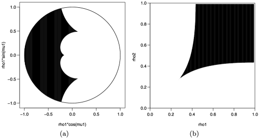
Figure 1: Discriminant $D$ as functions of: (a) $(\rho_{1}\cos\mu_{1},\rho_{1}\sin\mu_{1})$ with $\rho_{2}=0.5$, and (b) $(\rho_{1},\rho_{2})$ with $\mu_{1}=2\uppi/3$. Positive $D$, corresponding to bimodality, is displayed in black, and negative $D$, corresponding to unimodality, is exhibited in white.

Figure 1 exhibits areas of positivity (bimodality of density) and negativity (unimodality of density) of the discriminant $D$ for two pairs of parameters. Figure 1(a) suggests that density (2) with $\rho_{1}=0.5$ becomes unimodal for most cases when $-\uppi/2\leq\mu_{1}\leq\uppi/2$. It seems that bimodality is most likely to occur if $\uppi/2\leq\mu_{1}\leq 3\uppi/2$. The other frame of Figure 1 seems to show that distribution (2) with $\mu_{2}=2\uppi/3$ is bimodal if $\rho_{1}$ or $\rho_{2}$ is sufficiently large, and $\rho_{2}/\rho_{1}$ takes a value close to $1$. In particular, when $\rho_{1}=\rho_{2}$, the range of parameters corresponding to unimodality seems less wide than that when $\rho_{1}=a\rho_{2}$ with $a\neq 1$. As will be shown in Section 6.2, for $\mu_{1}=2\uppi/3$ and $\rho_{1}=\rho_{2}$, the density becomes unimodal if $\rho_{1}\leq 2-\sqrt{3}\simeq 0.268$ and bimodal otherwise.

Figure 2: Density (2) for $\mu_{2}=0$ and (a) $\rho_{1}=2/3,\ \rho_{2}=1/3$ and: $\mu_{1}=0$ (solid), $\uppi/3$ (dashed), $2\uppi/3$ (dot-dashed) and $\uppi$ (dotted), (b) $\mu_{1}=\uppi/2,\ \rho_{2}=1/3$ and: $\rho_{1}=0$ (solid), $1/4$ (dashed), $1/2$ (dot-dashed) and $3/4$ (dotted), (c) $\rho_{2}=1/3$ and: $(\mu_{1},\rho_{1})=(\uppi,1/3)$ (solid), $(0,0)$ (dashed), $(0,1/3)$ (dot-dashed) and $(0,2/3)$ (dotted), and (d) $\rho_{1}=\rho_{2}=0.5$ and: $\mu_{1}=0$ (solid), $\uppi/3$ (dashed), $2\uppi/3$ (dot-dashed) and $\uppi$ (dotted).

3.3 Pictures of density

We plot density (2) for selected values of the parameters in Figure 2. Confirming the results in the previous two subsections, this figure shows that the density can be symmetric or asymmetric, unimodal or bimodal, depending on the choice of the parameters. Figure 2(a), displaying the density for fixed values of $\mu_{2},\rho_{1}$ and $\rho_{2}$, suggests that the density is symmetric if $\mu_{1}=\mu_{2}$ or $\mu_{1}=\mu_{2}+\uppi$ and asymmetric otherwise. Figure 2(b) exhibits how the shape of density (2) changes as $\rho_{1}$ increases. It is clear from this frame that the greater the value of $\rho_{1}$, the greater the concentration of the density. The frame also implies that the absolute value of the circular skewness of the density with fixed $\mu_{1}$ and $\mu_{2}$ takes a large value if $\rho_{1}/\rho_{2}$ is close to 1. Some symmetric cases of the density are shown in Figure 2(c). It appears to be that the density is unimodal when $\mu_{1}=\mu_{2}$, whereas bimodality can occur when $\mu_{2}=\mu_{1}+\uppi$. Figure 2(d) is a case in which two parameters, $\rho_{1}$ and $\rho_{2}$, are fixed to be equal (to 0.5), also implying that density (2) is symmetric. We will focus on this submodel in Section 6.2.

4 Trigonometric moments and related problems

4.1 Trigonometric moments

It is often the case that asymmetric distributions on the circle have complicated trigonometric moments or Fourier coefficients. One feature of our asymmetric model, however, is the relative simplicity of its trigonometric moments. The expression for the moments is greatly simplified if the variables and parameters are represented in terms of complex numbers.

Theorem 4

Let a random variable $Z$ have the $\operatorname{EC}^{*}(\phi_{1},\phi_{2})$ distribution. Then the $n$th trigonometric moment of $Z$ is given by

$$E(Z^{n})=\cases{\displaystyle\frac{(1-|\phi_{2}|^{2})(1-\overline{\phi_{1}}\phi_{2})\phi_{1}^{n+1}-(1-|\phi_{1}|^{2})(1-\phi_{1}\overline{\phi_{2}})\phi_{2}^{n+1}}{(\phi_{1}-\phi_{2})(1-|\phi_{1}\overline{\phi_{2}}|^{2})},&\quad$\phi_{1}\neq\phi_{2}$,\cr\displaystyle\frac{1+n+(1-n)|\phi_{1}|^{2}}{1+|\phi_{1}|^{2}}\phi_{1}^{n},&\quad$\phi_{1}=\phi_{2}$.}$$

Proof.

The $n$th trigonometric moment can be expressed as

$$E(Z^{n}) = \frac{1}{2\uppi}\frac{|1-\overline{\phi_{1}}\phi_{2}|^{2}}{1-|\phi_{1}\overline{\phi_{2}}|^{2}}\int_{\partial D}z^{n}\Biggl{(}\prod_{j=1}^{2}\frac{1-|\phi_{j}|^{2}}{|z-\phi_{j}|^{2}}\Biggr{)}|\mathrm{d}z|$$

$$= \frac{1}{2\uppi\mathrm{i}}\frac{|1-\overline{\phi_{1}}\phi_{2}|^{2}}{1-|\phi_{1}\overline{\phi_{2}}|^{2}}\int_{\partial D}z^{n+1}\Biggl{\{}\prod_{j=1}^{2}\frac{1-|\phi_{j}|^{2}}{(z-\phi_{j})(1-\overline{\phi_{j}}z)}\Biggr{\}}\,\mathrm{d}z.$$

If $\phi_{1}\neq\phi_{2}$, the integrand in (4.1) is holomorphic on the unit disc, except at two poles of order 1, that is, $z=\phi_{j},\ j=1,2$. When $\phi_{1}=\phi_{2}$, the integrand in (4.1) has a single pole of order 2 at $z=\phi_{1}$. Hence, from the residue theorem (e.g., Rudin [18], Theorem 10.42), we obtain Theorem 4. ∎

4.2 Mean direction and mean resultant length

Let $Z$ be distributed as $\operatorname{EC}^{*}(\phi_{1},\phi_{2})$. From Theorem 4 it is easy to see that the first trigonometric moment for $Z$ is simply expressed as

$$E(Z)=\frac{(1-|\phi_{2}|^{2})\phi_{1}+(1-|\phi_{1}|^{2})\phi_{2}}{1-|\phi_{1}\phi_{2}|^{2}}\qquad\mbox{for any $\phi_{1}$ and $\phi_{2}$}.$$ (7)

The following result provides the condition under which the first trigonometric moment is equal to zero.

Corollary 0.

The necessary and sufficient condition for $E(Z)=0$ is given by $\phi_{1}=-\phi_{2}$.

Proof.

It is straightforward to show the sufficient condition for $E(Z)=0$. The necessary condition is proved as follows. Let $E(Z)=0$ and $\phi_{1}\neq-\phi_{2}$. Then, from Theorem 4, the following equation holds between the two parameters: $\phi_{1}\phi_{2}=({\phi_{1}+\phi_{2}})/{\overline{(\phi_{1}+\phi_{2})}}.$ Taking the absolute values of both sides of the above equation, we have $|\phi_{1}\phi_{2}|=1.$ Since $|\phi_{j}|<1\ (j=1,2)$, there does not exist $\phi_{1}$ and $\phi_{2}$ such that $|\phi_{1}\phi_{2}|=1$. Therefore, if $\phi_{1}\neq-\phi_{2}$, then $E(Z)\neq 0$. ∎

The mean direction is a measure of location which is defined as $\arg\{E(Z)\}$ if $E(Z)\neq 0$ and is undefined if $E(Z)=0$. The mean resultant length, which is a measure of concentration, is defined by $|E(Z)|$. Figure 3 shows the mean direction and mean resultant length of a random variable having density (3) with fixed $\phi_{2}=0.5$. Figure 3(a) suggests that the mean direction monotonically increases as $\arg(\phi_{1})$ increases from $-\uppi$ to $\uppi$. As seen in Corollary 1, Figure 3(b) confirms that the mean resultant length is zero if $\phi_{1}=-0.5$. It seems from this frame that unimodality holds for the mean resultant length as a function of $\phi_{1}$.

Figure 3: Plot of (a) mean direction and (b) mean resultant length of a random variable having the distribution $\operatorname{EC}^{*}(\phi_{1},0.5)$, as a function of $\phi_{1}$.

4.3 Skewness

A measure of skewness for circular distributions (Mardia [13]), $s$, is defined by

$$s={E[\operatorname{Im}\{(Z\mathrm{e}^{-\mathrm{i}\zeta})^{2}\}]}/{(1-\delta)^{3/2}},$$ (8)

where $\zeta$ and $\delta$ are the mean direction and mean resultant length for a $\partial D$-valued random variable $Z$, respectively. For our model, it is possible to express the skewness for the proposed model in a fairly simple form as follows.

Corollary 0.

Let $Z$ be distributed as $\operatorname{EC}^{*}(\phi_{1},\phi_{2})$. Then the skewness for the distribution of $Z$ is given by

$$s=\frac{|1-\phi_{1}\overline{\phi_{2}}|^{2}}{(1-|\phi_{1}\overline{\phi_{2}}|^{2})^{3}}\rho^{-2}(1-\rho)^{-3/2}\operatorname{Im}(\phi_{1}\overline{\phi_{2}})(|\phi_{1}|^{2}-|\phi_{2}|^{2})(1-|\phi_{1}|^{2})(1-|\phi_{2}|^{2}),$$ (9)

where $\rho=|(1-|\phi_{2}|^{2})\phi_{1}+(1-|\phi_{1}|^{2})\phi_{2}|/(1-|\phi_{1}\overline{\phi_{2}}|^{2}).$

Proof.

Note that the numerator of (8) can be expressed as

$$E[\operatorname{Im}\{(Z\mathrm{e}^{-\mathrm{i}\mu})^{2}\}]=\operatorname{Im}[E(Z^{2})\{\overline{E(Z)}/|E(Z)|\}^{2}].$$

Then, by using Theorem 4 and equation (7), the skewness (9) can be obtained after lengthy, but straightforward, calculations. ∎

Now we write $s=s(\phi_{1},\phi_{2})$ in order to view the skewness (9) as a function of $\phi_{1}$ and $\phi_{2}$. It follows from Corollary 2 and Theorem 3 that the following properties hold for $s$.

Theorem 5

The following properties hold for the skewness (9):

1. [5.]

2. $s(\phi_{1},\phi_{2})=0\Longleftrightarrow$ density (3) is symmetric.

3. $s(\phi_{1},\phi_{2})>0\ (<0)\Longleftrightarrow\operatorname{Im}(\phi_{1}\overline{\phi_{2}})(|\phi_{1}|-|\phi_{2}|)>0\ (<0).$

4. $s(\phi_{1},\phi_{2})=-s(\phi_{1},\overline{\phi_{2}}\phi_{1}^{2}/|\phi_{1}|^{2})=-s(\overline{\phi_{1}}\phi_{2}^{2}/|\phi_{2}|^{2},\phi_{2}),\phi_{1},\phi_{2}\neq 0$.

5. $s(\phi_{2},\phi_{1})=s(\phi_{1},\phi_{2})$.

6. $s(\overline{\phi_{1}},\overline{\phi_{2}})=-s(\phi_{1},\phi_{2}).$

7. $s(\alpha\phi_{1},\alpha\phi_{2})=s(\phi_{1},\phi_{2}),\alpha\in\partial D.$

8. Assume $\rho_{1},\rho_{2}>0$ and $\sin(\mu_{1}-\mu_{2})>0\ (<0)$. Then $\lim_{\rho_{1}\rightarrow 1}s(\rho_{1}\mathrm{e}^{\mathrm{i}\mu_{1}},\rho_{2}\mathrm{e}^{\mathrm{i}\mu_{2}})=\infty\ (-\infty)$.

Figure 4 plots this skewness when $\phi_{2}=0.5$. As the first property of Theorem 5 shows, the skewness is equal to zero if and only if $\operatorname{Im}(\phi_{1}\overline{\phi_{2}})=0,\ |\phi_{1}|=|\phi_{2}|$ or $|\phi_{j}|=0$ $(j=1,2)$. This figure also confirms the second property of Theorem 5 that the model is positively (negatively) skewed if $|\phi_{1}|>|\phi_{2}|$ and $\operatorname{Im}(\phi_{1}\overline{\phi_{2}})>0$ ($\operatorname{Im}(\phi_{1}\overline{\phi_{2}})<0$), or $|\phi_{1}|<|\phi_{2}|$ and $\operatorname{Im}(\phi_{1}\overline{\phi_{2}})<0$ ($\operatorname{Im}(\phi_{1}\overline{\phi_{2}})>0$). It can also be seen that the fifth and seventh properties of Theorem 5 hold in this figure.

Figure 4: Skewness (9) of a random variable having the distribution $\operatorname{EC}^{*}(\phi_{1},0.5)$, as a function of $\phi_{1}$.

5 Some other topics

5.1 Alternative derivations

As discussed in Section 2.1, the proposed model can be derived by considering a problem in Brownian motion. Apart from the derivation given there, here is another method to generate our family via this stochastic process, kindly suggested by the referee.

Remember that, given a $\mathbb{C}$-valued Brownian path without drift starting from $\phi$ $(\in D)$, the point of first exit from the unit disc $D$ has a wrapped Cauchy distribution with density proportional to $1/|z-\phi|^{2}$. (Although we assume $\phi\in D$ by convention, the Brownian motion starting at $1/\overline{\phi}$ has the same hitting distribution from the exterior because of the conformal invariance of Brownian motion.) From this it follows that another derivation of the proposed model (3) is given in the following theorem.

Theorem 6

Let $Z_{1}$ and $Z_{2}$ be the points of first exit from the unit disc for two independent $\mathbb{C}$-valued Brownian motions without drift starting from $\phi_{1}$ and $\phi_{2}$, respectively, where $\phi_{1},\phi_{2}\in D$. Then the conditional distribution of $Z_{1}$ $(\equiv Z)$ given $Z_{1}=Z_{2}$ is given by density (3).

Remark 0.

The referee embedded the above in a generalized formulation leading to densities of the form

$$f(z)\propto\prod_{j=1}^{d}\frac{1-|\phi_{j}|^{2}}{|z-\phi_{j}|^{2}},\qquad z\in\partial D;\phi_{1},\ldots,\phi_{d}\in D,$$ (10)

many of whose properties are also readily obtainable using the residue theorem.

In addition to the derivations using Brownian motion, there are other methods to generate our family. The following result shows that the proposed model appears in a Bayesian context.

Theorem 7

Let $\Theta|\nu$ have the wrapped Cauchy distribution $\operatorname{WC}(\nu,\rho_{1})$ with known $\rho_{1}$. Assume that the prior distribution of $\nu$ is distributed as the wrapped Cauchy $\operatorname{WC}(\mu_{2},\rho_{2})$. Then the posterior distribution of $\nu$ given $\Theta=\mu_{1}$ has density (2).

The above derivation enables us to generate random samples from our model using the Markov chain Monte Carlo method; see Kato and Jones [10], Section 5.3, for details.

Remark 0.

In Theorem 7, the marginal distribution of $\Theta$ is given by the wrapped Cauchy distribution, $\operatorname{WC}(\mu_{1}+\mu_{2},\rho_{1}\rho_{2})$.

Before we discuss a third method to derive our model, here we briefly recall a known property of the wrapped Cauchy distribution or the Poisson kernel as follows.

Theorem 8 ((Rudin [18], Theorem 11.9))

Assume $\overline{D}$ is the closed unit disc in the complex plane. Suppose a function $u$ is continuous on $\overline{D}$ and harmonic in $D$, and suppose that $|u(z)|<\infty$ for any $z\in\overline{D}$. Then

$$\int_{\partial D}u(z)\frac{1}{2\uppi}\frac{1-|\phi_{1}|^{2}}{|z-\phi_{1}|^{2}}\,\mathrm{d}z=u(\phi_{1}),\qquad\phi_{1}\in D.$$

Note that the integrand in the left-hand side of the above equation is actually the product of $u(z)$ and the density of the wrapped Cauchy $C^{*}(\phi_{1})$. From the fact that

$$g(z)=\frac{|\phi_{2}^{-1}|^{2}-|z|^{2}}{|z-\overline{\phi_{2}}^{-1}|^{2}},\qquad\phi_{2}\in D,$$

is a continuous real function on $\overline{D}$ and harmonic in $D$, it follows that

$$f(z)=\frac{g(z)}{2\uppi g(\phi_{1})}\frac{1-|\phi_{1}|^{2}}{|z-\phi_{1}|^{2}},\qquad z\in\partial D,$$

satisfies the definition of a density. Clearly, $f(z)$ is equal to density (3).

The following theorem implies that our model appears as a special case of a further general family of distributions. The proof is straightforward and omitted.

Theorem 9

Let $f$ and $g$ be probability density functions on the circle. Assume that $h$ is the convolution of $f$ and $g$, namely, $h(\tau)=(f*g)(\tau)=\int_{-\uppi}^{\uppi}f(\theta)g(\tau-\theta)\,\mathrm{d}\theta$. Then a function $k(\theta)=f(\theta)g(\tau-\theta)/h(\tau)$ is a probability density function on the circle.

Density (2) can be derived on setting $\tau=\mu_{2}$ and $f$ and $g$ as the densities of $\operatorname{WC}(\mu_{1},\rho_{1})$ and $\operatorname{WC}(0,\rho_{2})$, respectively. In this case $h(\tau)$ also has the form of the wrapped Cauchy density $\operatorname{WC}(\mu_{1},\rho_{1}\rho_{2})$ since the wrapped Cauchy distribution has the additive property.

5.2 Möbius transformation

The Möbius transformation is well known in complex analysis as a conformal mapping which projects the unit disc onto itself. It is defined as

$${\cal{M}}(w)=\alpha\frac{w+\beta}{\overline{\beta}w+1},\qquad w\in\overline{D};\alpha\in\partial D,\beta\in D.$$

Although this projection is usually defined on the interior of the unit disc, here we extend the domain of the mapping so that the boundary of the unit disc, that is, the unit circle, is included. It is easy to see that the unit circle is mapped onto itself via the transformation, namely, ${\cal M}(\partial D)=\partial D$. In directional statistics the transformation appears in some papers such as McCullagh [15], Jones [6] and Kato and Jones [9].

Here we study the conformal invariance properties of our family. The distribution (3) has a density that is a relative invariant of weight 2 in the sense that

$$f(z;\phi_{1},\phi_{2})=f\{{\cal M}(z);{\cal M}(\phi_{1}),{\cal M}(\phi_{2})\}|{\cal M}^{\prime}(z)|^{2}.$$

Similarly, the extended family (10) has a density that is relatively invariant with weight $k$, in the sense that $f(z;\phi_{1},\ldots,\phi_{k})=f\{{\cal M}(z);{\cal M}(\phi_{1}),\ldots,{\cal M}(\phi_{k})\}|{\cal M}^{\prime}(z)|^{k}.$ The relative invariance with weight 1 of the wrapped Cauchy distribution can be obtained by putting $k=1$.

The proposed family (3) is not closed under the Möbius transformation except for the wrapped Cauchy special cases. To say the same thing in a different way, if $Z$ follows the distribution (3), then the density for ${\cal M}(Z)$ is not of the form (3) except for $\phi_{1}=0$ or $\phi_{2}=0$. This fact can be understood clearly in the following context; as seen in Theorem 6, our model (3) can be derived as the conditional distribution of $Z_{1}$ given $Z_{1}=Z_{2}$, where $Z_{1}$ and $Z_{2}$ are independent wrapped Cauchy variables. Invertibility of the transformations ${\cal M}$ implies that $Z_{1}=Z_{2}$ if and only if ${\cal M}(Z_{1})={\cal M}(Z_{2})$. However, as is known as the Borel paradox (e.g., Pollard [17], Section 5.5), the conditional distribution of $Z_{1}$ given $Z_{1}=Z_{2}$ is generally not the same as the conditional distribution of $Z_{1}$ given ${\cal M}(Z_{1})={\cal M}(Z_{2})$. Consequently, the Möbius transformation of the conditional distribution of $Z_{1}$ given $Z_{1}=Z_{2}$, which is the Möbius transformation of model (3), is not the same as the conditional distribution of ${\cal M}(Z_{1})$ given ${\cal M}(Z_{1})={\cal M}(Z_{2})$, which is model (3). In a similar manner one can see that the extended model (10) with $k\geq 2$ is not closed under the Möbius transformation.

6 Symmetric cases

So far, we have mostly considered the full family of distributions with densities (2) and (3). In this section, we focus on the symmetric special cases of the proposed model. Some properties, which the general family does not have, hold for the symmetric cases. In Section 6.1, model (2) with $\mu_{1}=\mu_{2}$ or $\mu_{2}+\uppi$ is discussed. In Section 6.2, we briefly consider another symmetric model, namely, model (2) with $\rho_{1}=\rho_{2}$.

6.1 Symmetric case I: $\mu_{1}=\mu_{2}$ or $\mu_{1}=\mu_{2}+\uppi$

Model (2) with $\mu_{1}=\mu_{2}$ or $\mu_{1}=\mu_{2}+\uppi$ is essentially the same as the distribution with density

$$f(\theta)=\frac{1-\rho_{1}\rho_{2}}{2\uppi(1+\rho_{1}\rho_{2})}\frac{1-\rho_{1}^{2}}{1+\rho_{1}^{2}-2\rho_{1}\cos(\theta-\mu)}\frac{1-\rho_{2}^{2}}{1+\rho_{2}^{2}-2\rho_{2}\cos(\theta-\mu)},$$

(11)

$$\quad-\uppi\leq\theta<\uppi,$$

where $-1<\rho_{1}<1,\ 0\leq\rho_{2}<1,$ and $-\uppi\leq\mu<\uppi$. Note the extension in the range of $\rho$: this density corresponds to (2) with $\mu_{1}=\mu_{2}$ when $\rho_{1}\geq 0$ in (6.1), while the density is equivalent to (2) with $\mu_{1}=\mu_{2}+\uppi$ when $\rho_{1}<0$ in (6.1). Clearly, the density is symmetric about $\theta=\mu$ and $\theta=\mu+\uppi$.

One might, however, wish to restrict interest to the case where $0\leq\rho_{1}<1$ because then density (6.1) is unimodal. To see this, note that in this case $a_{0}=a_{1}=a_{4}=0$ in (5) so that stationary points of the density occur at $\sin\theta=0$ and, potentially, also at $\cos\theta=-a_{2}/a_{3}=(\rho_{1}+\rho_{2})(1+\rho_{1}\rho_{2})/4\rho_{1}\rho_{2}$. However, the latter expression can easily be proved to not be less than unity, showing that (6.1) is unimodal. On the other hand, the symmetric model (6.1) with negative $\rho_{1}$ has a relationship with mixtures of two wrapped Cauchy distributions. The density for this submodel can be expressed as

$$f(\theta) = p\frac{1}{2\uppi}\frac{1-\rho_{1}^{2}}{1+\rho_{1}^{2}-2\rho_{1}\cos(\theta-\mu)}+(1-p)\frac{1}{2\uppi}\frac{1-\rho_{2}^{2}}{1+\rho_{2}^{2}-2\rho_{2}\cos(\theta-\mu)},$$

where $p=-\rho_{1}(1-\rho_{2}^{2})/\{(1+\rho_{1}\rho_{2})(\rho_{2}-\rho_{1})\}$. Inter alia, this representation allows random numbers from density (6.1) with $\rho_{1}\leq 0$ to be more easily generated than they were for the general case in Kato and Jones [10], Section 5.3.

6.2 Symmetric case II: $\rho_{1}=\rho_{2}$

In this section we discuss the submodel of density (2) with $\rho_{1}=\rho_{2}=\rho\ (\in[0,1))$. The density for this submodel reduces to

$$f(\theta) = \frac{(1-\rho^{2})\{1+\rho^{4}-2\rho^{2}\cos(\mu_{1}-\mu_{2})\}}{2\uppi(1+\rho^{2})}$$

$${}\times[\{1+\rho^{2}-2\rho\cos(\theta-\mu_{1})\}\{1+\rho^{2}-2\rho\cos(\theta-\mu_{2})\}]^{-1},\qquad-\uppi\leq\theta<\uppi.$$

The model is symmetric about $\theta=\overline{\mu}$ and $\overline{\mu}+\uppi$, where $\overline{\mu}=\arg(\sum_{j=1}^{2}\cos\mu_{j}+\mathrm{i}\sum_{j=1}^{2}\sin\mu_{j})$. As displayed in Figure 2(d), this submodel can be unimodal or bimodal depending on the choice of the parameters. The condition for unimodality can be simplified for this submodel as follows:

$$-2\arccos\biggl{(}\frac{2\rho}{1+\rho^{2}}\biggr{)}\leq\mu_{1}-\mu_{2}\leq 2\arccos\biggl{(}\frac{2\rho}{1+\rho^{2}}\biggr{)}.$$

This result was used in Section 3.2 to find the region of Figure 1(b) in which the discriminant takes negative values, corresponding to unimodality, when $\rho_{1}=\rho_{2}$ and $\mu_{1}-\mu_{2}=2\uppi/3$.

7 A generalization on the sphere

As described in Section 2.1, the proposed model (2) can be derived using Brownian motion. By adopting a multi-dimensional Brownian motion instead of the two-dimensional one, we can extend model (2) to a distribution on the unit sphere. The generalized model is defined as follows.

Definition 2.

Let $\{B_{t};t\geq 0\}$ be $\mathbb{R}^{d}$-valued Brownian motion starting at $B_{0}=\rho_{1}\eta_{1}$, where $d\geq 2$, $0\leq\rho_{1}<1,\ \eta_{1}\in S^{d}$ and $S^{d}=\{x\in\mathbb{R}^{d};\|x\|=1\}$. Assume $\tau_{1}=\inf\{t;\|B_{t}\|=1\}$ and $\tau_{2}=\inf\{t;\|B_{t}\|=\rho_{2}^{-1}\}$, where $0<\rho_{2}<1$. Then the proposed model is defined by the conditional distribution of $B_{\tau_{1}}$ given $B_{\tau_{2}}=\rho_{2}^{-1}\eta_{2},$ where $\eta_{2}\in S^{d}$.

For simplicity, write $X=B_{\tau_{1}}$. The probability density function of this extended model is available, and it is given in the following theorem.

Theorem 10

The conditional distribution of $X$ given $B_{\tau_{2}}=\rho_{2}^{-1}\eta_{2}$ is of the form

$$f(x)=\frac{1}{A_{d-1}}\frac{(1+\rho_{1}^{2}\rho_{2}^{2}-2\rho_{1}\rho_{2}\eta_{1}^{\prime}\eta_{2})^{d/2}}{1-\rho_{1}^{2}\rho_{2}^{2}}\frac{1-\rho_{1}^{2}}{\|x-\rho_{1}\eta_{1}\|^{d}}\frac{1-\rho_{2}^{2}}{\|x-\rho_{2}\eta_{2}\|^{d}},\qquad x\in S^{d},$$ (12)

where $A_{d-1}$ is the surface area of $S^{d}$, that is, $A_{d-1}=2\uppi^{d/2}/\Gamma(d/2)$.

See Appendix C of Kato and Jones [10] for the proof. Note that density (12) reduces to the circular case (2) if $d=2,\ x=(\cos\theta,\sin\theta)^{\prime},\ \eta_{1}=(\cos\mu_{1},\sin\mu_{1})^{\prime}$ and $\eta_{2}=(\cos\mu_{2},\sin\mu_{2})^{\prime}$. It might be appealing that density (12), which is not rotationally symmetric in general, can be expressed in a relatively simple form.

When $\rho_{2}=0$, the distribution becomes the so-called “exit” distribution on the sphere, whose density is given by

$$f(x)=\frac{1}{A_{d-1}}\frac{1-\rho_{1}^{2}}{\|x-\rho_{1}\eta_{1}\|^{d}},\qquad x\in S^{d}.$$ (13)

We write $X\sim\operatorname{Exit}_{d}(\rho_{1}\eta_{1})$ if a random variable $X$ has density (13). This model is rotationally symmetric about $x=\eta_{1}$. See, for example, Durrett [3], Section 1.10, for details about the distribution. In particular, when $d=2$, model (13) becomes the wrapped Cauchy distribution. It is noted that this distribution is a submodel of Jones and Pewsey’s [7] family of distributions on the sphere with density

$$f(x)=\frac{1}{A_{d-1}}\frac{|\sinh(\kappa\psi)|^{d/2-1}}{2^{2/d-1}\Gamma(d/2)}\frac{\{\cosh(\kappa\psi)+\sinh(\kappa\psi)x^{\prime}\mu\}^{1/\psi}}{P_{1/\psi+d/2-1}^{1-d/2}\{\cosh(\kappa\psi)\}},\qquad x\in S^{d},$$ (14)

where $P_{\alpha}^{\beta}(z)$ is the associated Legendre function of the first kind of degree $\alpha$ and order $\beta$ (Gradshteyn and Ryzhik [5], Sections 8.7, 8.8). It follows from equation (8.711.1) of Gradshteyn and Ryzhik [5] and equation (2) of McCullagh [14] that density (14) reduces to density (13) if $\kappa=d\log\{(1+\rho_{1})/(1-\rho_{1})\}/2,\ \mu=\eta_{1}$ and $\psi=-2/d$. Also, the extended model (12) includes the model with density

$$f(x)=\frac{1}{A_{d-1}}\frac{(1-\rho_{1}^{2})^{d+1}}{1+\rho_{1}^{2}}\frac{1}{\|x-\rho_{1}\eta_{1}\|^{2d}},\qquad x\in S^{d},$$ (15)

when $\rho_{1}=\rho_{2},\ \eta_{1}=\eta_{2}$. It can be seen that this model is another submodel of Jones and Pewsey’s [7] family (14) by putting $\psi=-1/d$ and $\kappa=d\log\{(1+\rho_{1})/(1-\rho_{1})\}$. Also, notice that, if $d=2$, density (15) corresponds to Case 2, (4), of circular submodels in Section 2.4. In addition to these two submodels, the multivariate model (12) contains the uniform distribution ($\rho_{1}=\rho_{2}=0$), one-point distribution ($\rho_{1}=0$ and $\rho_{2}\rightarrow 1$, or $\rho_{2}=0$ and $\rho_{1}\rightarrow 1$), and two-point distribution ($\rho_{1}=\rho_{2},\ \mu_{1}\neq\mu_{2}$ and $\rho_{1}\rightarrow 1$).

In a similar manner to Theorem 7, it is easy to prove that model (12) can be derived from Bayesian analysis of the exit distribution.

Theorem 11

Let $X|\xi$ be distributed as the exit distribution $\operatorname{Exit}(\rho_{1}\xi)$ with known $\rho_{1}$. Suppose that the prior distribution of $\xi$ is $\operatorname{Exit}(\rho_{2}\eta_{2})$. Then the posterior distribution of $\xi$ given $X=\eta_{1}$ is given by density (12).

From this result and the random number generator of the exit distribution given by Kato [8], Section 3.3, it is possible to generate random samples from (12) through the Markov chain Monte Carlo method in a similar manner to Kato and Jones [10], Section 5.3.

References

• [1] {bmisc}[auto:STB—2011/12/15—13:36:40] \bauthor\bsnmAbramowitz, \bfnmM.\binitsM. &\bauthor\bsnmStegun, \bfnmI. A.\binitsI.A. (\byear1970). \bhowpublishedHandbook of Mathematical Functions. New York: Dover Press. \bptokimsref \endbibitem
• [2] {bbook}[mr] \bauthor\bsnmBatschelet, \bfnmEduard\binitsE. (\byear1981). \btitleCircular Statistics in Biology. \baddressLondon: \bpublisherAcademic Press. \bidmr=0659065 \bptokimsref \endbibitem
• [3] {bbook}[mr] \bauthor\bsnmDurrett, \bfnmRichard\binitsR. (\byear1984). \btitleBrownian Motion and Martingales in Analysis. \bseriesWadsworth Mathematics Series. \baddressBelmont, CA: \bpublisherWadsworth International Group. \bidmr=0750829 \bptokimsref \endbibitem
• [4] {barticle}[mr] \bauthor\bsnmGatto, \bfnmRiccardo\binitsR. &\bauthor\bsnmJammalamadaka, \bfnmSreenivasa Rao\binitsS.R. (\byear2007). \btitleThe generalized von Mises distribution. \bjournalStat. Methodol. \bvolume4 \bpages341–353. \biddoi=10.1016/j.stamet.2006.11.003, issn=1572-3127, mr=2380560 \bptokimsref \endbibitem
• [5] {bbook}[mr] \bauthor\bsnmGradshteyn, \bfnmI. S.\binitsI.S. &\bauthor\bsnmRyzhik, \bfnmI. M.\binitsI.M. (\byear2007). \btitleTable of Integrals, Series, and Products, \bedition7th ed. \baddressAmsterdam: \bpublisherElsevier/Academic Press. \bnoteTranslated from the Russian. Translation edited and with a preface by Alan Jeffrey and Daniel Zwillinger. \bidmr=2360010 \bptokimsref \endbibitem
• [6] {barticle}[mr] \bauthor\bsnmJones, \bfnmM. C.\binitsM.C. (\byear2004). \btitleThe Möbius distribution on the disc. \bjournalAnn. Inst. Statist. Math. \bvolume56 \bpages733–742. \biddoi=10.1007/BF02506486, issn=0020-3157, mr=2126808 \bptokimsref \endbibitem
• [7] {barticle}[mr] \bauthor\bsnmJones, \bfnmM. C.\binitsM.C. &\bauthor\bsnmPewsey, \bfnmArthur\binitsA. (\byear2005). \btitleA family of symmetric distributions on the circle. \bjournalJ. Amer. Statist. Assoc. \bvolume100 \bpages1422–1428. \biddoi=10.1198/016214505000000286, issn=0162-1459, mr=2236452 \bptokimsref \endbibitem
• [8] {barticle}[mr] \bauthor\bsnmKato, \bfnmShogo\binitsS. (\byear2009). \btitleA distribution for a pair of unit vectors generated by Brownian motion. \bjournalBernoulli \bvolume15 \bpages898–921. \biddoi=10.3150/08-BEJ178, issn=1350-7265, mr=2555204 \bptokimsref \endbibitem
• [9] {barticle}[mr] \bauthor\bsnmKato, \bfnmShogo\binitsS. &\bauthor\bsnmJones, \bfnmM. C.\binitsM.C. (\byear2010). \btitleA family of distributions on the circle with links to, and applications arising from, Möbius transformation. \bjournalJ. Amer. Statist. Assoc. \bvolume105 \bpages249–262. \biddoi=10.1198/jasa.2009.tm08313, issn=0162-1459, mr=2656051 \bptokimsref \endbibitem
• [10] {bmisc}[auto:STB—2011/12/15—13:36:40] \bauthor\bsnmKato, \bfnmS.\binitsS. &\bauthor\bsnmJones, \bfnmM. C.\binitsM.C. (\byear2011). \bhowpublishedAn extended family of circular distributions related to wrapped Cauchy distributions via Brownian motion. Technical Report 11/02, Statistics Group, The Open Univ. Available at http://statistics.open.ac.uk. \bptokimsref \endbibitem
• [11] {barticle}[auto:STB—2011/12/15—13:36:40] \bauthor\bsnmKent, \bfnmJ. T.\binitsJ.T. &\bauthor\bsnmTyler, \bfnmD. E.\binitsD.E. (\byear1988). \btitleMaximum likelihood estimation for the wrapped Cauchy distribution. \bjournalJ. Appl. Statist. \bvolume15 \bpages247–254. \bptokimsref \endbibitem
• [12] {barticle}[mr] \bauthor\bsnmMaksimov, \bfnmV. M.\binitsV.M. (\byear1967). \btitleNecessary and sufficient statistics for a family of shifts of probability distributions on continuous bicompact groups. \bjournalTeor. Verojatnost. i Primenen. \bvolume12 \bpages307–321 \bnote(in Russian). English translation: Theor. Probab. Appl. 12 267–280. \bidissn=0040-361X, mr=0214175 \bptokimsref \endbibitem
• [13] {bbook}[mr] \bauthor\bsnmMardia, \bfnmK. V.\binitsK.V. (\byear1972). \btitleStatistics of Directional Data. \baddressLondon: \bpublisherAcademic Press. \bidmr=0336854 \bptokimsref \endbibitem
• [14] {barticle}[mr] \bauthor\bsnmMcCullagh, \bfnmPeter\binitsP. (\byear1989). \btitleSome statistical properties of a family of continuous univariate distributions. \bjournalJ. Amer. Statist. Assoc. \bvolume84 \bpages125–129. \bidissn=0162-1459, mr=0999670 \bptokimsref \endbibitem
• [15] {barticle}[mr] \bauthor\bsnmMcCullagh, \bfnmPeter\binitsP. (\byear1996). \btitleMöbius transformation and Cauchy parameter estimation. \bjournalAnn. Statist. \bvolume24 \bpages787–808. \biddoi=10.1214/aos/1032894465, issn=0090-5364, mr=1394988 \bptokimsref \endbibitem
• [16] {barticle}[mr] \bauthor\bsnmPewsey, \bfnmArthur\binitsA. (\byear2008). \btitleThe wrapped stable family of distributions as a flexible model for circular data. \bjournalComput. Statist. Data Anal. \bvolume52 \bpages1516–1523. \biddoi=10.1016/j.csda.2007.04.017, issn=0167-9473, mr=2422752 \bptokimsref \endbibitem
• [17] {bbook}[mr] \bauthor\bsnmPollard, \bfnmDavid\binitsD. (\byear2002). \btitleA User’s Guide to Measure Theoretic Probability. \bseriesCambridge Series in Statistical and Probabilistic Mathematics \bvolume8. \baddressCambridge: \bpublisherCambridge Univ. Press. \bidmr=1873379 \bptokimsref \endbibitem
• [18] {bbook}[mr] \bauthor\bsnmRudin, \bfnmWalter\binitsW. (\byear1987). \btitleReal and Complex Analysis, \bedition3rd ed. \baddressNew York: \bpublisherMcGraw-Hill. \bidmr=0924157 \bptokimsref \endbibitem
• [19] {bbook}[auto:STB—2011/12/15—13:36:40] \bauthor\bsnmUspensky, \bfnmJ. V.\binitsJ.V. (\byear1948). \btitleTheory of Equations. \baddressNew York: \bpublisherMcGraw-Hill. \bptokimsref \endbibitem
• [20] {barticle}[auto:STB—2011/12/15—13:36:40] \bauthor\bsnmYfantis, \bfnmE. A.\binitsE.A. &\bauthor\bsnmBorgman, \bfnmL. E.\binitsL.E. (\byear1982). \btitleAn extension of the von Mises distribution. \bjournalComm. Statist. Theory Methods \bvolume11 \bpages1695–1706. \bptokimsref \endbibitem