Abstract

‘Distribution regression’ refers to the situation where a response $Y$ depends on a covariate $P$ where $P$ is a probability distribution. The model is $Y=f(P)+\mu$ where $f$ is an unknown regression function and $\mu$ is a random error. Typically, we do not observe $P$ directly, but rather, we observe a sample from $P$. In this paper we develop theory and methods for distribution-free versions of distribution regression. This means that we do not make distributional assumptions about the error term $\mu$ and covariate $P$. We prove that when the effective dimension is small enough (as measured by the doubling dimension), then the excess prediction risk converges to zero with a polynomial rate.

1 Introduction

In a standard regression model, we need to predict a real-valued response $Y$ from a vector-valued covariate (or feature) $X\in\mathbb{R}^{d}$. Recently, there has been interest in extensions of standard regression from finite dimensional Euclidean spaces to other domains. For example, in functional regression (Ferraty and Vieu (2006)) the covariate is a function instead of a finite dimensional vector.

In this paper, we study distribution regression where the covariate is a probability distribution $P$. This differs from functional regression in two important ways. First, $P$ is a probability measure on $\mathbb{R}^{k}$ rather than a one-dimensional function. Second, and more importantly, we do not observe the covariate $P$ directly. Rather, we observe a sample from $P$, which means that we have a regression model with measurement error (Carroll et al. (2006), Fan and Truong (1993)).

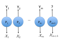
Figure 1: Illustration of the model - distributions $P_{1},\dots,P_{m},P_{m+1}$ are unobserved, only the ${\cal X}_{1},\ldots,{\cal X}_{m},{\cal X}_{m+1}$ sample sets are observable.

The formal definition of the problem is as follows. We consider a regression problem with variables $(P_{1},Y_{1}),\ldots,(P_{m},Y_{m})$ where $Y_{i}\in\mathbb{R}$ and each $P_{i}$ is a probability distribution on a compact subset ${\cal K}\subset\mathbb{R}^{k}$. We assume that

$$Y_{i}=f(P_{i})+\mu_{i},\quad i=1,\ldots,m,$$

for some functional $f$, where $\mu_{i}$ is a noise variable with mean 0. We do not observe $P_{i}$ directly; rather we observe a sample

$$X_{i1},\ldots,X_{in_{i}}\stackrel{{\scriptstyle i.i.d}}{{\sim}}P_{i}.$$ (1)

Thus the observed data are

$$({\cal X}_{1},Y_{1}),\ldots,({\cal X}_{m},Y_{m})$$ (2)

where ${\cal X}_{i}=\{X_{i1},\ldots,X_{in_{i}}\}$. Our goal is to predict a new $Y_{m+1}$ from a new batch ${\cal X}_{m+1}$ drawn from a new distribution $P_{m+1}$. This model is illustrated in Figure 1.

We model the unobservable probability distributions $P_{1},\ldots,P_{m}$ as follows. Let $\mathbb{D}$ denote the set of all distributions on ${\cal K}$ that have a density with respect to the Lebesgue measure. We assume that the distributions $P_{i}$ are an i.i.d. sample from a measure ${\cal P}$ on $\mathbb{D}$, that is,

$$P_{1},\ldots,P_{m},P_{m+1}\stackrel{{\scriptstyle i.i.d}}{{\sim}}{\cal P}.$$

Note that $f:\mathbb{D}\to\mathbb{R}$. If $Q(\cdot|P)$ denotes the law of $Y$ given $P$, then the joint distribution of $(Y,P)$ is given by

$$\mathbb{P}(Y\in A,P\in B) =Q(Y\in A|P\in B)\mathcal{P}(P\in B)$$

Our main result is a theorem where we prove that when the effective dimension measured by the doubling dimension is small enough, then the estimator is consistent and the prediction risk converges to zero with a polynomial rate.

Our results are distribution free in the sense that the only distributional assumptions we make in this regression problem are that $\mu_{i}$ has mean 0 and that $\mathbb{P}(|Y_{i}|\leq B_{Y})=1$ for some $B_{Y}$. We make no other distributional assumptions.

Outline. In Section 2 we discuss related work. We propose a specific estimator for distribution regression in Section 3. We call this kernel-kernel estimator since it makes use of kernels in two different ways. In Section 4 we derive an upper bound on the risk of the estimator. The proofs can be found in Section 5. In Section 6 we analyze the risk bound in terms of the doubling dimension, which is a measure of the intrinsic dimension of the space. We present numerical illustrations in Section 7. Finally, we give some concluding remarks in Section 8.

2 Related work

Our framework is related to functional data analysis, which is a new and steadily improving field of statistics. For comprehensive reviews and references, see Ramsay and Silverman (2005); Ferraty and Vieu (2006).

A popular approach to do machine learning, such as classification and regression, on the domain of distributions is to embed the distribution to a Hilbert space, introduce kernels between the distributions, and then use a traditional kernel machine to solve the learning problem. There are both parametric and nonparametric methods proposed in the literature.

Parametric methods, (e.g. Jebara et al. (2004); Moreno et al. (2004); Jaakkola and Haussler (1998)), usually fit a parametric family (e.g. Gaussians distributions or exponential family) to the densities, and using the fitted parameters they estimate the inner products between the distributions. The problem with parametric approaches, however, is that when the true densities do not belong to the assumed parametric families, then this method introduces some unavoidable bias during the estimation of the inner products between the densities.

A couple of nonparametric approaches exist as well. Since our covariates are represented by finite sets, reproducing kernel Hilbert space (RKHS) based set kernels can be used in these learning problems. Smola et al. (2007) proposed to embed the distributions to an RKHS using the mean map kernels. In this framework, the role of universal kernels have been studied by Christmann and Steinwart (2010). Recently, the representer theorem has also been generalized for the space of probability distributions (Muandet et al., 2012). Kondor and Jebara (2003) introduced Bhattacharyya’s measure of affinity between finite-dimensional Gaussians in a Hilbert space. In contrast to the previous approaches, Póczos et al. (2012, 2011) used nonparametric Rényi divergence estimators to solve machine learning problems on the set of distributions.

Although, there are a few algorithms designed for regression on distributions, we know very little about their theoretical properties. To the best of our knowledge, even the simplest, fundamental questions have not been studied yet. For example, we do not know how many distributions ($m$) and how many samples ($n_{i}$, $i=1,\ldots,m$) we need to achieve small prediction error. Our paper is providing an answer to this question.

3 The Kernel-Kernel Estimator

In this section we define an estimator $\widehat{f}$ for the unknown function $f$. Our predictor for $Y_{m+1}$ is then $\widehat{Y}_{m+1}=\widehat{f}({\cal X}_{m+1})$. Let $\widehat{P}_{i}$ denote an estimator of $P_{i}$ based on ${\cal X}_{i}$, and let ${\cal X}$ be a sample from a new distribution $P=P_{m+1}$. Accordingly, we denote with $\widehat{P}$ an estimator of $P$ based on ${\cal X}$.

Given a bandwidth $h>0$ and a kernel function $K$ (whose properties will be specified later), we define

$$\widehat{f}(\widehat{P}) =\widehat{f}(\widehat{P};\widehat{P}_{1},\ldots,\widehat{P}_{m})$$

$$=\begin{cases}\frac{\sum_{i}Y_{i}K\left(\frac{D(\widehat{P}_{i},\widehat{P})}{h}\right)}{\sum_{i}K\left(\frac{D(\widehat{P}_{i},\widehat{P})}{h}\right)}&\mbox{if }\sum_{i}K\left(\frac{D(\widehat{P}_{i},\widehat{P})}{h}\right)>0\\ 0&\mbox{otherwise.}\end{cases}$$

To complete the definition, we need to specify $\widehat{P}_{i}$, $\widehat{P}$ and $D$. We will estimate $P_{i}$ — or, more precisely, the density $p_{i}$ of $P_{i}$ — with a kernel density estimator

$$\widehat{p}_{i}(x)=\frac{1}{n_{i}}\sum_{j=1}^{n_{i}}\frac{1}{b_{i}^{k}}B\left(\frac{\|x-X_{ij}\|}{b_{i}}\right)$$ (3)

where $B$ is an appropriate kernel function (see, e.g. Tsybakov (2010)) with bandwidth $b_{i}>0$. Here $\|x\|$ denotes the Euclidean norm of $x\in\mathbb{R}^{k}$. Accordingly, $\widehat{P}_{i}$ is defined by

$$\widehat{P}_{i}(A)=\int_{A}\widehat{p}_{i}(u)du,$$

for all Borel measurable subsets of $\mathbb{R}^{k}$. For any two probabilities in $P$ and $Q$ in $\mathbb{D}$, we take $D(P,Q)$ to be the $L_{1}$ distance of their densities: $D(P,Q)=\|p-q\|=\int|p(x)-q(x)|dx$. Hence,

$$\widehat{f}(\widehat{P})=\widehat{f}(\widehat{P};\widehat{P}_{1},\ldots,\widehat{P}_{m})=\frac{\sum_{i=1}^{m}Y_{i}K\left(\frac{||\widehat{p}-\widehat{p}_{i}||}{h}\right)}{\sum_{i=1}^{m}K\left(\frac{||\widehat{p}-\widehat{p}_{i}||}{h}\right)}$$ (4)

which we call the ‘kernel-kernel estimator’ since it makes use of two kernels, $B$ and $K$.

For simplicity, $n$ will denote the size of the sample $\mathcal{X}$, and $b$ will be the bandwidth in the estimator of $\widehat{p}$.

In what follows we will make the following assumptions on $f$, $K$, $\mathcal{P}$, $\mu_{i}$, and $Y_{i}$.

Assumptions

• (A1) Hölder continuous functional. The unknown functional $f$ belongs to the class ${\cal M}={\cal M}(L,\beta,D)$ of Hölder continuous functionals on $\mathbb{D}$:

  $${\cal M}=\Biggl{\{}f:\ |f(P_{i})-f(P_{j})|\leq L\,D(P_{i},P_{j})^{\beta}\Biggr{\}},$$

  for some $L>0$ and $0<\beta\leq 1$, where $D$ is the above specified $L_{1}$ metric on $\mathbb{D}$. In the $\beta=1$ special case this means that $f$ is Lipschitz continuous.

• (A2) Asymmetric boxed and Lipschitz kernel. The kernel $K$ satisfies the following properties: $K:[0,\infty]\to\mathbb{R}$ is non-negative and Lipschitz continuous with Lipschitz constant $L_{K}$. In addition, there exist constants $0<\underline{K}<1$ and $0<r<R<\infty$ such that, for all $x>0$, it holds that

  $$\underline{K}I_{\{x\in\mathcal{B}(0,r)\}}\leq K(x)\leq I_{\{x\in\mathcal{B}(0,R)\}}.$$

• (A3) Hölder class of distributions. The distribution ${\cal P}$ is supported on the set of distributions ${\cal H}_{k}(1)$ with densities that are $1$-smooth Hölder functions, as defined in Rigollet and Vert (2009).

• (A4) Bounded regression. We will assume that ${\sup}_{P\in\mathcal{P}}|f(P)|<f_{\max}$ for some $f_{\max}>0$. Also, $\mu_{i}$ has mean $0$ and $\mathbb{P}(|Y_{i}|\leq B_{Y})=1$ for some $B_{Y}<\infty$.

• (A5) Lower bound on $\min_{1\leq i\leq m+1}{n_{i}}$. Let $n=\min_{1\leq i\leq m+1}{n_{i}}$. We assume that $e^{n^{\frac{k}{2+k}}}/m\to\infty$ as $m\to\infty$.

• (A6) Relationship between $n$ and $h$. Assume that $C_{*}n^{-\frac{1}{2+k}}\leq rh/4$ where $C_{*}$ is defined in (9).

4 Upper Bound on Risk

We are concerned with upper bounding the risk

$$R(m,n)=\mbox{$\mathbb{E}$}\bigg{[}|\widehat{f}(\widehat{P};\widehat{P}_{1},\ldots,\widehat{P}_{m})-f(P)|\bigg{]},$$

where the expectation is with respect to the joint distribution of the sample $({\cal X}_{1},Y_{1}),\ldots,({\cal X}_{m},Y_{m})$, the new covariate $P=P_{m+1}$ and the new observation ${\cal X}_{m+1}$. Note that the absolute prediction risk is $\mathbb{E}|\widehat{Y}-Y|\leq R(m,n)+c$, where $c=\mathbb{E}(|\mu|)$ is a constant. So bounding the prediction risk is equivalent to bounding $R(m,n)$, which we call the excess prediction risk. In what follows, $C,c_{1},c_{2},\ldots$ represent constants whose value can be different in different expressions.

Let $\mathcal{B}(P,h)=\{\widetilde{P}\in\mathbb{D}:D(\widetilde{P},P)\leq h\}$ denote the $L_{1}$ ball of distributions around $P$ with radius $h$. We will see that the risk depends on the size of the class of probabilities $\mathbb{D}$. In particular, the risk depends on the small ball probability

$$\Phi_{P}(h)=\mathcal{P}(\mathcal{B}(P,h)),$$

where $P$ is a fixed distribution and $\Phi_{P}(h)$ is a function of $P$.

Our first result, Theorem 1, provides a general upper bound on the risk. In our second result (Section 6) we show that when the effective dimension measured by the doubling dimension is small, then the risk converges to zero. We also derive an upper bound on the rate of convergence.

Theorem 1

Suppose that the assumptions stated above hold. Let $b=n^{-\frac{1}{2+k}}$ be the bandwidth in the density estimators $\widehat{p}_{i}$. Then

$$R (m,n)\leq\frac{1}{h}\mbox{$\mathbb{E}$}\left[\frac{1}{\Phi_{P}(rh/2)}\right]C_{1}n^{-\frac{1}{2+k}}+C_{2}h^{\beta}$$

$$+C_{3}\sqrt{\frac{1}{m}}\sqrt{\mbox{$\mathbb{E}$}\left[\frac{1}{\Phi_{P}(rh/2)}\right]}+{\frac{C_{4}}{m}}{\mbox{$\mathbb{E}$}\left[\frac{1}{\Phi_{P}(rh/2)}\right]}$$

$$+(m+1)e^{-\frac{1}{2}n^{\frac{k}{2+k}}},$$

where the constants $C_{i}$’s are specified in the proof.

5 Proof of Theorem 1

In this Section we prove our main result, Theorem 1. The main idea of the proof is to use the triangle inequality to write

$$R(m,n) =\mbox{$\mathbb{E}$}|\widehat{f}(\widehat{P};\widehat{P}_{1},\ldots,\widehat{P}_{m})-f(P)|$$

$$\leq\mbox{$\mathbb{E}$}|\widehat{f}(\widehat{P};\widehat{P}_{1},\ldots,\widehat{P}_{m})-\widehat{f}(P;P_{1},\ldots,P_{m})|$$ (5)

$$\qquad+\mbox{$\mathbb{E}$}|\widehat{f}(P;P_{1},\ldots,P_{m})-f(P)|.$$ (6)

In Sections 5.2 and 5.3 we will derive upper bounds for (5) and (6), respectively. Section 5.1 contains a series of technical results needed in our proofs.

Throughout, we let $\widehat{K}_{i}=K\left(\frac{D(\widehat{P}_{i},\widehat{P})}{h}\right)$, $K_{i}=K\left(\frac{D(P_{i},P)}{h}\right)$ and $\epsilon_{i}=K_{i}-\widehat{K}_{i}$, for $i=1,\ldots,m$. Note that, for ease of readability, we have omitted the dependence on $h$.

5.1 Technical Results

5.1.1 $L_{1}$ Risk of Density Estimators

In this section we bound $\mbox{$\mathbb{E}$}[D(P,\widehat{P})|P]=\mbox{$\mathbb{E}$}[\int|p-\widehat{p}||P]$, the $L_{1}$ risk of the density estimator $\widehat{p}$ of $p$, uniformly over all $P$ in $\mathbb{D}$. To this end, suppose that $n_{i}\geq n$ for all $i=1,2,\ldots,m+1$, and let $b_{i}=b=n^{-\frac{1}{k+2}}$. In this case, the following lemma provides upper bound on the $L_{1}$ risk of the density estimator.

Lemma 2

$$\mbox{$\mathbb{E}$}[D(\widehat{P}_{i},P_{i})|P_{i}] \leq\bar{C}n^{-\frac{1}{2+k}},$$ (7)

$$\mbox{$\mathbb{E}$}[D(\widehat{P}_{i},P_{i})] \leq\bar{C}n^{-\frac{1}{2+k}},$$

where

$$\bar{C}=c_{0}(c_{1}+c_{2}),$$ (8)

with $c_{0}$, $c_{1}$ and $c_{1}$ constants specified in the proof.

Proof. Recall that we assume that ${\cal P}$ is supported on the set ${\cal H}_{k}(1)$ of distributions, which are $1$-smooth $k$-dimensional densities as defined in Rigollet and Vert (2009).

Let $\mbox{$\mathbb{E}$}\bigg{[}D_{2}(\widehat{P}_{i},P)|P_{i}\bigg{]}=\mbox{$\mathbb{E}$}\bigg{[}\sqrt{\int(\widehat{p}_{i}-p_{i})^{2}}\bigg{]}$ denote the integrated mean squared risk for the density estimator $\widehat{p}_{i}$ of a fixed density $p_{i}$. It then follows from Lemma 4.1 of Rigollet and Vert (2009) that (with an appropriate kernel function $B$),

$$\mbox{$\mathbb{E}$}[D^{2}_{2}(\widehat{P}_{i},P_{i})|P_{i}] \leq c_{1}^{2}b_{i}^{2}+\left(\frac{c_{2}^{2}}{n_{i}b_{i}^{k}}\right)$$

for some constants $c_{1},c_{2}>0$.

From Jensen’s inequality, we have that $E[X]\leq(\mbox{$\mathbb{E}$}[X^{2}])^{1/2}$ for any $X$ random variable. We also know that $(a+b)^{1/2}\leq a^{1/2}+b^{1/2}$ for any $a,b>0$, therefore

$$\mbox{$\mathbb{E}$}[D_{2}(\widehat{P}_{i},P_{i})|P_{i}] \leq\left(c_{1}^{2}b_{i}^{2}+\left(\frac{c_{2}^{2}}{n_{i}b_{i}^{k}}\right)\right)^{1/2}$$

$$\leq c_{1}b_{i}+\frac{c_{2}}{n_{i}^{1/2}b_{i}^{k/2}}.$$

Since the distributions in $\mathbb{D}$ are supported on a compact set and the kernel $B$ has also compact support, we have, for an appropriate constant $c_{0}>0$,

$$\int|p_{i}-\widehat{p}_{i}|\leq c_{0}\sqrt{\int(p_{i}-\widehat{p}_{i})^{2}}.$$

Therefore,

$$\mbox{$\mathbb{E}$}[D(\widehat{P}_{i},P_{i})|P_{i}] \leq c_{0}\mbox{$\mathbb{E}$}[D_{2}(\widehat{P}_{i},P_{i})|P_{i}]$$

$$\leq c_{0}(c_{1}b_{i}+\frac{c_{2}}{n_{i}^{1/2}b_{i}^{k/2}})$$

$$\leq c_{0}(c_{1}+c_{2})n^{-\frac{1}{2+k}},$$

where the last step follows from our assumptions that $n_{i}^{-1/2}b_{i}^{-k/2}\leq n^{-\frac{1}{2}}n^{\frac{k}{2(k+2)}}=n^{-\frac{1}{k+2}}$, and thus

$$c_{1}b_{i}+\frac{c_{2}}{n_{i}^{1/2}b_{i}^{k/2}}\leq(c_{1}+c_{2})n^{-\frac{1}{2+k}}.$$

$\Box$

Next, we show that the terms $D(\widehat{P}_{i},P_{i})$ are uniformly bounded by a term of order $O(h)$, with high probability.

Lemma 3

With probability no smaller than $1-(m+1)e^{-\frac{1}{2}n^{\frac{k}{2+k}}}$, $D(\widehat{P}_{i},P_{i})<\frac{rh}{4}$ for all $i=1,\ldots,m+1$.

Notice that by Assumption (A5), $1-(m+1)e^{-\frac{1}{2}n^{\frac{k}{2+k}}}\rightarrow 1$.

Proof. From McDiarmid’s inequality, for any $\epsilon>0$ we have that

$$\mathbb{P}(||\widehat{p}_{i}-p_{i}||_{1}-\mathbb{E}||\widehat{p}_{i}-p_{i}||_{1}>\epsilon)\leq e^{-n\epsilon^{2}/2}$$

(see, for example, section 2.4 of Devroye and Lugosi (2001)). Thus,

$$\mathbb{P}(||\widehat{p}_{i}-p_{i}||_{1}>\mathbb{E}||\widehat{p}_{i}-p_{i}||_{1}+n^{-\frac{1}{2+k}}) \leq e^{-\frac{1}{2}n^{\frac{k}{2+k}}},$$

since $nn^{-\frac{2}{2+k}}=n^{\frac{k}{2+k}}$. This implies that

$$\mathbb{P}(\max_{1\leq i\leq m+1}||\widehat{p}_{i}-p_{i}||_{1}>\mathbb{E}||\widehat{p}_{i}-p_{i}||_{1}+n^{-\frac{1}{2+k}}))$$

$$\leq(m+1)e^{-\frac{1}{2}n^{\frac{k}{2+k}}}\to 0,$$

by assumption (A5). Therefore,

$$1 -(m+1)e^{-\frac{1}{2}n^{\frac{k}{2+k}}}$$

$$\leq\mathbb{P}(\max_{1\leq i\leq m+1}||\widehat{p}_{i}-p_{i}||_{1}\leq\mathbb{E}||\widehat{p}_{i}-p_{i}||_{1}+n^{-\frac{1}{2+k}}))$$

$$\leq\mathbb{P}(\max_{1\leq i\leq m+1}||\widehat{p}_{i}-p_{i}||_{1}\leq(1+c_{0}(c_{1}+c_{2}))n^{-\frac{1}{2+k}}).$$

This implies that with

$$C_{*}=(1+c_{0}(c_{1}+c_{2}))$$ (9)

and using assumption (A6), we have that

$$D(\widehat{P}_{i},P_{i})\leq C_{*}n^{-\frac{1}{k+2}}\leq\frac{rh}{4}\ \ \ {\rm for\ all\ }i$$ (10)

on an event $\Omega_{m,n}$, where $\mathbb{P}(\Omega_{m,n}^{c})\leq(m+1)e^{-\frac{1}{2}n^{\frac{k}{2+k}}}$. Here $\Omega_{m,n}^{c}$ denotes the complement of $\Omega_{m,n}$. $\Box$

5.1.2 Other Lemmata

Throughout this section we will make use of the constant $\bar{C}$, defined in (8). In what follows, we will need a few lemmas that we list below. Their proofs can be found in the supplementary material.

The following lemma provides an upper bound on $\mathbb{P}(\sum_{i=1}^{m}K_{i}=0)$ with the help of small ball probabilities.

Lemma 4

$$\mathbb{P}\Bigl{(}\sum_{i=1}^{m}K_{i}=0\Bigr{)} \leq\mathbb{P}\Bigl{(}\sum_{i=1}^{m}K_{i}<\underline{K}\Bigr{)}=\frac{1}{em}\mathbb{E}\left[\frac{1}{\Phi_{P}(rh)}\right].$$

We will also need the following lemma.

Lemma 5

$$\mbox{$\mathbb{E}$}\left[\frac{1}{\sum_{i}K_{i}}I_{\{\sum_{i}K_{i}\geq\underline{K}\}}\right]\leq\frac{1+1/\underline{K}}{m\underline{K}}\mbox{$\mathbb{E}$}\bigg{[}\frac{1}{\Phi_{P}(Rh)}\bigg{]}.$$

The following lemma provides an upper bound on $|\epsilon_{i}|$.

Lemma 6

Assume that the kernel function $K$ is Lipschitz continuous with Lipschitz constant $L_{K}$. We have that

$$|\epsilon_{i}| \leq\frac{L_{K}}{h}({D(P,\widehat{P})}+{D(P_{i},\widehat{P}_{i})}).$$

By definition, $|\epsilon_{i}|=|K_{i}-\widehat{K}_{i}|=|K(\frac{D(P,P_{i})}{h})-K(\frac{D(\widehat{P},\widehat{P}_{i})}{h})|$, which is a deterministic function of random variables $P$, $P_{i}$, $\widehat{P}$, and $\widehat{P}_{i}$. We will denote this deterministic relationship as $\epsilon_{i}=\epsilon_{i}(P,\widehat{P},P_{i},\widehat{P}_{i})$. The following lemma shows that for any $\kappa>0$,

$$\mathbb{P}\Bigl{(}\sum_{i}|\epsilon_{i}(P,\widehat{P},P_{i},\widehat{P}_{i})|<\kappa|\{P_{i}\}_{i=1}^{m},P\Bigr{)}$$

can be lower bounded by a non-trivial quantity that does not depend on $P$ and $\{P_{i}\}_{i=1}^{m}$.

Lemma 7

For any $\kappa>0$ we have that

$$\mathbb{P} (\sum_{i}|\epsilon_{i}(P,\widehat{P},P_{i},\widehat{P}_{i})|<\kappa|\{P_{i}\}_{i=1}^{m},P)\geq\eta,$$

where $\eta=\eta(\kappa,n,m)=1-\frac{2L_{K}m\bar{C}}{h\kappa}n^{-\frac{1}{2+k}}$.

The following lemma provides an upper bound on the expected value of $\sum_{i=1}^{m}|\epsilon_{i}|$.

Lemma 8

$$\mathbb{E} \left[\sum_{i=1}^{m}|\epsilon_{i}|\bigg{|}P,\{P_{i}\}_{i=1}^{m}\right]\leq\frac{2L_{K}\bar{C}m}{h}n^{-\frac{1}{2+k}}.$$

The next lemma shows that $\mathbb{P}\Bigl{(}\sum_{i=1}^{m}\widehat{K}_{i}<\underline{K}\Bigr{)}$ can be upper bounded by a small quantity as well. We assume that $n_{i}=n$ and $b_{i}=b$ for all $i$. Define

$$\zeta =\zeta(n,m)=\frac{1}{em}\mathbb{E}\left(\frac{1}{\Phi_{P}\left(\frac{rh}{2}\right)}\right)+(m+1)e^{-\frac{1}{2}n^{\frac{k}{2+k}}}.$$

Lemma 9

$$\mathbb{P}\Bigl{(}\sum_{i=1}^{m}\widehat{K}_{i}=0\Bigr{)}\leq\mathbb{P}\Bigl{(}\sum_{i=1}^{m}\widehat{K}_{i}<\underline{K}\Bigr{)}\leq\zeta.$$

5.2 Upper bound on Equation 5

Let $\Delta\widehat{f}=|\widehat{f}(\widehat{P};\widehat{P}_{1},\ldots,\widehat{P}_{m})-\widehat{f}(P;P_{1},\ldots,P_{m})|$. Our goal is to provide an upper bound on $\mbox{$\mathbb{E}$}[\Delta\widehat{f}]$.

Introduce the following events: $E_{0}=\{\sum_{i}K_{i}=0\}$, $E_{1}=\{0<\sum_{i}K_{i}<\underline{K}\}$, $E_{2}=\{\underline{K}\leq\sum_{i}K_{i}\}$. Similarly, $\widehat{E}_{0}=\{\sum_{i}\widehat{K}_{i}=0\}$, $\widehat{E}_{1}=\{0<\sum_{i}\widehat{K}_{i}<\underline{K}\}$, $\widehat{E}_{2}=\{\underline{K}\leq\sum_{i}\widehat{K}_{i}\}$. Obviously, $\mbox{$\mathbb{E}$}[\Delta\widehat{f}]=\sum_{k=0}^{2}\sum_{l=0}^{2}\mbox{$\mathbb{E}$}[\Delta\widehat{f}I_{E_{k}}I_{\widehat{E}_{l}}].$

Based on the sign of $\sum_{i}K_{i}$ and $\sum\widehat{K}_{i}$, there are four different cases. (i) If $\sum_{i}K_{i}>0$ and $\sum_{i}\widehat{K}_{i}>0$, then $\Delta\widehat{f}=|\frac{\sum_{i}Y_{i}\widehat{K}_{i}}{\sum_{i}\widehat{K}_{i}}-\frac{\sum_{i}Y_{i}K_{i}}{\sum_{i}K_{i}}|$. (ii) If $\sum_{i}K_{i}>0$ and $\sum_{i}\widehat{K}_{i}=0$, then $\Delta\widehat{f}=|\frac{\sum_{i}Y_{i}K_{i}}{\sum_{i}K_{i}}|$. (iii) If $\sum_{i}K_{i}=0$ and $\sum_{i}\widehat{K}_{i}>0$, then $\Delta\widehat{f}=|\frac{\sum_{i}Y_{i}\widehat{K}_{i}}{\sum_{i}\widehat{K}_{i}}|$, and finally (iv) if $\sum_{i}K_{i}=0$ and $\sum_{i}\widehat{K}_{i}=0$, then $\Delta\widehat{f}=0$. From this it immediately follows that $\mbox{$\mathbb{E}$}[\Delta\widehat{f}I_{E_{0}}I_{\widehat{E}_{0}}]=0$.

When $\sum_{i}K_{i}>0$, $\left|\sum_{i}\frac{Y_{i}K_{i}}{\sum_{i}K_{i}}\right|\leq B_{Y}$. Therefore,

$$\mathbb{E} \left[\left|\sum_{i}\frac{Y_{i}K_{i}}{\sum_{i}K_{i}}\right|I_{\widehat{E}_{0}}(I_{E_{1}}+I_{E_{2}})\right]$$

$$\qquad\leq B_{Y}\mbox{$\mathbb{E}$}\left[I_{\{\sum_{i}K_{i}>0\wedge\sum_{i}\widehat{K}_{i}=0\}}\right]$$

$$\qquad=B_{Y}\mathbb{P}(\sum_{i}K_{i}>0,\sum_{i}\widehat{K}_{i}=0)$$

$$\qquad\leq B_{Y}\mathbb{P}(\sum_{i=1}^{m}\widehat{K}_{i}=0)\leq B_{Y}\zeta(n,m).$$

Similarly,

$$\mathbb{E} \left[\left|\sum_{i}\frac{Y_{i}\widehat{K}_{i}}{\sum_{i}\widehat{K}_{i}}\right|I_{E_{0}}(I_{\widehat{E}_{1}}+I_{\widehat{E}_{2}})\right]\leq\frac{B_{Y}}{em}\int\frac{d{\mathcal{P}}(P)}{{\Phi}_{P}(rh)}.$$

It is also easy to see that

$$\mathbb{E} \left[\Delta\widehat{f}I_{E_{1}}(I_{\widehat{E}_{1}}+I_{\widehat{E}_{2}})\right]$$

$$\leq\mbox{$\mathbb{E}$}\bigg{[}\left(\left|\sum_{i}\frac{Y_{i}K_{i}}{\sum_{i}K_{i}}\right|+\left|\sum_{i}\frac{Y_{i}\widehat{K}_{i}}{\sum_{i}\widehat{K}_{i}}\right|\right)I_{E_{1}}(I_{\widehat{E}_{1}}+I_{\widehat{E}_{2}})\bigg{]}$$

$$\leq\mbox{$\mathbb{E}$}\bigg{[}2B_{Y}I_{E_{1}}(I_{\widehat{E}_{1}}+I_{\widehat{E}_{2}})\bigg{]}\leq 2B_{Y}\mbox{$\mathbb{E}$}\bigg{[}I_{E_{1}}\bigg{]}$$

$$=2B_{Y}\mathbb{P}(\sum_{i=1}^{m}0<K_{i}<\underline{K}/2)\leq\frac{2B_{Y}}{em}\int\frac{d\mathcal{P}(P)}{{\Phi}_{P}(rh)}.$$

Similarly,

$$\mbox{$\mathbb{E}$}\left[\Delta\widehat{f}I_{\widehat{E}_{1}}(I_{E_{1}}+I_{E_{2}})\right] \leq 2B_{Y}\mathbb{P}(\sum_{i=1}^{m}0<\widehat{K}_{i}<\underline{K}/2)$$

$$\leq 2B_{Y}\zeta(n,m).$$

All that left is to upper bound $\mbox{$\mathbb{E}$}\left[\Delta\widehat{f}I_{E_{2}}I_{\widehat{E}_{2}}\right]$. The next lemma provides an upper bound for this.

Lemma 10

$$\mathbb{E} \left[\Delta\widehat{f}I_{E_{2}}I_{\widehat{E}_{2}}\right]\leq C_{1}\frac{1}{h}\mbox{$\mathbb{E}$}\bigg{[}\frac{1}{\Phi_{P}(Rh)}\bigg{]}n^{-\frac{1}{2+k}}.$$

The proof can be found in the supplementary material.

Finally, putting the pieces together we obtain the following theorem.

Theorem 11

$$\mathbb{E} |\widehat{f}(\widehat{P};\widehat{P}_{1},\ldots,\widehat{P}_{m})-\widehat{f}(P;P_{1},\ldots,P_{m})|$$

$$\leq C_{1}\frac{1}{h}\mbox{$\mathbb{E}$}\bigg{[}\frac{1}{\Phi_{P}(rh/2)}\bigg{]}n^{-\frac{1}{2+k}}+C_{2}\frac{1}{m}\mathbb{E}\left[\frac{1}{\Phi_{P}(rh/2)}\right]$$

$$\qquad+(m+1)e^{-\frac{1}{2}n^{\frac{k}{2+k}}}.$$

The proof can be found in the supplementary material.

5.3 Upper bound on Equation 6

In this section we show that under the above specified conditions $\mbox{$\mathbb{E}$}|\widehat{f}(P;P_{1},\ldots,P_{m})-f(P)|$ can be upper bounded by

$$C_{1}(h^{\beta})+C_{2}\left(\sqrt{\mbox{$\mathbb{E}$}\left[\frac{1}{m\Phi_{P}(rh/2)}\right]}\right)+{\frac{C_{3}}{m}\mbox{$\mathbb{E}$}\left[\frac{1}{\Phi_{P}(rh/2)}\right]},$$

where the expectation is with respect to the random probability measure $P$ in $\mathcal{P}$.

We have to bound $\mbox{$\mathbb{E}$}|\widehat{f}(P;P_{1},\ldots,P_{m})-f(P)|$. Note that $Y_{i}=f(P_{i})+\mu_{i}$, and

$$\mbox{$\mathbb{E}$}|\widehat{f} (P;P_{1},\ldots,P_{m})-f(P)|$$

$$=\mbox{$\mathbb{E}$}\left|\frac{\sum_{i}Y_{i}K_{i}}{\sum_{i}K_{i}}I_{\{\sum_{i}K_{i}>0\}}-f(P)\right|$$

$$=\mbox{$\mathbb{E}$}\left|\frac{\sum_{i}(f(P_{i})+\mu_{i})K_{i}}{\sum_{i}K_{i}}I_{\{\sum_{i}K_{i}>0\}}-f(P)\right|$$

$$\leq\mbox{$\mathbb{E}$}\left[\left|\frac{\sum_{i}(f(P_{i})-f(P))K_{i}}{\sum_{i}K_{i}}+\frac{\sum_{i}\mu_{i}K_{i}}{\sum_{i}K_{i}}\right|I_{\{\sum_{i}K_{i}>0\}}\right]$$

$$\quad+\mbox{$\mathbb{E}$}\left[\left|f(P)\right|I_{\{\sum_{i}K_{i}=0\}}\right|$$

$$\leq\mbox{$\mathbb{E}$}\left[\frac{\sum_{i}|f(P_{i})-f(P)|K_{i}}{\sum_{i}K_{i}}I_{\{\sum_{i}K_{i}>0\}}\right]$$

$$\quad+\mbox{$\mathbb{E}$}\left[\left|\frac{\sum_{i}\mu_{i}K_{i}}{\sum_{i}K_{i}}\right|I_{\{\sum_{i}K_{i}>0\}}\right]+f_{\max}\mathbb{P}(\sum_{i}K_{i}=0).$$

We will bound each of the three terms next. For the first term, since $f$ is Hölder-$\beta$ we have

$$\mathbb{E} \left[\frac{\sum_{i}|f(P_{i})-f(P)|K_{i}}{\sum_{i}K_{i}}I_{\{\sum_{i}K_{i}>0\}}\right]$$

$$\leq\mbox{$\mathbb{E}$}\left[\frac{\sum_{i}LD(P_{i},P)^{\beta}K_{i}}{\sum_{i}K_{i}}I_{\{\sum_{i}K_{i}>0\}}\right]\leq L\,(hR)^{\beta},$$

where in the last step we used the fact that

$$D(P_{i},P)^{\beta}K_{i}=D(P_{i},P)^{\beta}K\left(\frac{D(P_{i},P)}{h}\right)\leq(hR)^{\beta}K_{i},$$

since $supp(K)\subseteq B(0,R)$.

We now bound the second term.

$$\mathbb{E} \left[\left|\frac{\sum_{i}\mu_{i}K_{i}}{\sum_{i}K_{i}}\right|I_{\{\sum_{i}K_{i}>0\}}\right]$$

$$=\mbox{$\mathbb{E}$}\left[\left|\frac{\sum_{i}\mu_{i}K_{i}}{\sum_{i}K_{i}}\right|I_{\{\sum_{i}K_{i}\geq\underline{K}\}}+\left|\frac{\sum_{i}\mu_{i}K_{i}}{\sum_{i}K_{i}}\right|I_{\{\underline{K}>\sum_{i}K_{i}>0\}}\right]$$

$$\leq\mbox{$\mathbb{E}$}\left[\left|\frac{\sum_{i}\mu_{i}K_{i}}{\sum_{i}K_{i}}\right|I_{\{\sum_{i}K_{i}\geq\underline{K}\}}\right]+B_{Y}\mbox{$\mathbb{P}$}(\underline{K}>\sum_{i}K_{i})$$

$$\leq\mbox{$\mathbb{E}$}\left[\left|\frac{\sum_{i}\mu_{i}K_{i}}{\sum_{i}K_{i}}\right|I_{\{\sum_{i}K_{i}\geq\underline{K}\}}\right]+\frac{B_{Y}}{em}\int\frac{d\mathcal{P}(P)}{\Phi_{P}(rh)}.$$

(A4) implies that $\mathbb{P}(|\mu_{i}|\leq B_{Y})=1$, i.e. $B_{Y}$ is a bound on the noise. The last step follows from Lemma 4. For the first term in the above expression, we use the following lemma. Its proof can be found in the supplementary material.

Lemma 12

$$\mbox{$\mathbb{E}$}\left[\left|\frac{\sum_{i}\mu_{i}K_{i}}{\sum_{i}K_{i}}\right|I_{\{\sum_{i}K_{i}\geq\underline{K}\}}\right]\leq B_{Y}\sqrt{\frac{1+1/\underline{K}}{m\underline{K}}\ \int\frac{d\mathcal{P}(P)}{\Phi_{P}(Rh)}}.$$

Finally, we bound the third term using Lemma 4:

$$f_{\max}\mathbb{P}(\sum_{i}K_{i}=0)\leq\frac{f_{\max}}{em}\int\frac{d\mathcal{P}(P)}{\Phi_{P}(rh)}.$$

Putting everything together, we have

$$\mathbb{E} |\widehat{f}(P;P_{1},\ldots,P_{m})-f(P)|$$

$$\leq L(hR)^{\beta}+B_{Y}\sqrt{\frac{1+1/\underline{K}}{m\underline{K}}\ \int\frac{d\mathcal{P}(P)}{\Phi_{P}(Rh)}}$$

$$\quad+\frac{B_{Y}}{em}\int\frac{d\mathcal{P}(P)}{\Phi_{P}(rh)}+\frac{f_{\max}}{em}\int\frac{d\mathcal{P}(P)}{\Phi_{P}(rh)}$$

$$\leq C_{1}h^{\beta}+C_{2}\sqrt{\frac{1}{m}\mbox{$\mathbb{E}$}\left[\frac{1}{\Phi_{P}(rh/2)}\right]}+{\frac{C_{3}}{m}\mbox{$\mathbb{E}$}\left[\frac{1}{\Phi_{P}(rh/2)}\right]}.$$

Note that $\Phi_{P}(rh/2)\leq\Phi_{P}(rh)\leq\Phi_{P}(Rh)$.

6 Doubling Dimension

The upper bound on the risk in Theorem 1 depends on the quantity $\mbox{$\mathbb{E}$}\bigg{[}\frac{1}{\Phi_{P}(rh/2)}\bigg{]}.$ In future work, we will show that, without further assumptions, this quantity can be quite large which leads to very slow rates of convergence. This is because the covering number of the class ${\cal H}_{k}(1)$ is huge. For this paper, we concentrate on the more optimistic case where the support of ${\cal P}$ has small effective dimension.

One way to measure effective dimension is to use the doubling dimension. Following Kpotufe (2011), we say that ${\cal P}$ is a doubling measure with effective dimension $d$ if, for every $r>0$ and $0<\epsilon<1$,

$$\frac{{\cal P}({\cal B}(s,r))}{{\cal P}({\cal B}(s,\epsilon r))}\leq\left(\frac{c}{\epsilon}\right)^{d}.$$ (11)

If $d$ denotes the doubling dimension of measure $\mathcal{P}$, then the $\sqrt{\mbox{$\mathbb{E}$}[1/(m\Phi_{P}(rh/2))]}$ term in Theorem 1 can be upper bounded as follows:

$$\sqrt{\mbox{$\mathbb{E}$}\bigg{[}\frac{1}{m\Phi_{P}(rh/2)}}\bigg{]}=\sqrt{\mbox{$\mathbb{E}$}\bigg{[}\frac{1}{m}\frac{\Phi_{P}(1)}{\Phi_{P}(rh/2)}\frac{1}{\Phi_{P}(1)}\bigg{]}}$$

$$\leq\sqrt{\frac{1}{m}C(rh/2)^{-d}\mbox{$\mathbb{E}$}\bigg{[}\frac{1}{\Phi_{P}(1)}\bigg{]}}\leq\frac{C}{\sqrt{mh^{d}}}.$$

Note also that when $mh^{d}\leq 1$, then $\frac{1}{mh^{d}}\leq\frac{1}{\sqrt{mh^{d}}}$. In this case, as a corollary of Theorem 1, we now have that

$$R(m,n)\leq\frac{C_{1}}{h^{d+1}n^{1/(k+2)}}+C_{2}h^{\beta}+C_{3}\sqrt{\frac{1}{mh^{d}}},\\$$ (12)

for appropriate constants $C_{1}$, $C_{2}$ and $C_{3}$.

To derive the rates for the risk, we consider two separate cases, depending on whether the third term in the right hand side of (12) dominates the first term or not.

Thus first assume that

$$\sqrt{\frac{1}{mh^{d}}}=\Omega\left(\frac{C_{1}}{h^{d+1}n^{1/(k+2)}}\right),$$ (13)

so that the risk becomes, asymptotically, $O\left(h^{\beta}+\sqrt{\frac{1}{mh^{d}}}\right)$. The optimal choice for $h$ is then $\Theta\left(m^{-1/(2\beta+d)}\right)$, yielding a rate for the risk

$$R(m,n)=O\left(m^{-\beta/(2\beta+d)}\right).$$

Notice that this choice of $h$ ensures that our assumption (A6) is met, since in this case (13) implies that

$$n=\Omega\left(m^{\frac{\beta+d+1}{2\beta+d}(k+2)}\right),$$

from which we obtain that

$$h=\Theta\left(m^{-\frac{1}{2\beta+d}}\right)=\Omega\left(n^{-\frac{1}{(k+2)(\beta+d+1)}}\right)=\Omega\left(n^{-\frac{1}{k+2}}\right).$$

This rate is reasonable because if the number of samples per distribution $n$ is large compared to the number $m$ of distributions, then the learning rate is limited by the number of distributions $m$ and is in fact precisely the same as the rate of learning a standard $\beta$-Hölder smooth regression function in $d$ dimensions. That is, the the effect of not knowing the distributions $P_{1},\dots,P_{m}$ exactly and only having a finite sample from the distributions is negligible.

For the second case, suppose that

$$\sqrt{\frac{1}{mh^{d}}}=O\left(\frac{1}{h^{d+1}n^{1/(k+2)}}\right).$$ (14)

Then, $R(m,n)=O\left(\frac{1}{h^{d+1}n^{1/(k+2)}}+h^{\beta}\right)$, which implies that the optimal choice for $h$ is $h=\Theta\left(n^{-\frac{1}{(k+2)(\beta+d+1)}}\right)$, giving the rate

$$R(m,n)=O\left(n^{-\frac{\beta}{(k+2)(\beta+d+1)}}\right).$$

Just like before, this choice of $h$ does not violate assumption (A6) since

$$h=\Theta\left(n^{-\frac{1}{(k+2)(\beta+d+1)}}\right)=\Omega\left(n^{-\frac{1}{k+2}}\right).$$

Notice that, (14) also implies that

$$m=\Omega\left(n^{\frac{2\beta+d}{(k+2)(\beta+d+1)}}\right).$$

In this case, the rate is limited by the number of samples per distribution $n$, as expected. Notice that the rate gets worse as the dimensionality of each distribution $k$ grows and as the smoothness $\beta$ of the regression function deteriorates.

Remark. If there is no additive noise, i.e. $\mu_{i}=0$, similar calculations yield that $R(m,n)=O\left(m^{-\frac{1}{\beta+d}}\right)$ when $n=\Omega\left(m^{\frac{\beta+d+1}{(\beta+d)(k+2)}}\right)$, and $R(m,n)=O\left(n^{-\frac{\beta}{(k+2)(\beta+d+1)}}\right)$ otherwise. While the rates seem reasonable, establishing optimality of the rates by demonstrating matching lower bounds is an open question that we plan to investigate in future work.

7 Numerical Illustrations

The following experiments serve as a proof of concepts to demonstrate the applicability of the distribution regression estimator in Section 3. In these experiments, we used triangle kernels ($k(x)=1-|x|$ if $-1\leq x\leq 1$, and $0$ otherwise). We set all the $n,n_{1},\ldots,n_{m}$ set sizes and $b,b_{1},\ldots,b_{m}$ bandwidths to the same values, which will be specified below. In the first experiment, we generated 325 sample sets from $Beta(a,3)$ distributions where $a$ was varied between $[3,20]$ randomly. We constructed $m=250$ sample sets for training, 25 for validation, and 50 for testing. Each sample set contained $n=500$ $Beta(a,3)$ distributed i.i.d. points. Our task in this experiment was to learn the skewness of $Beta(a,b)$ distributions, $f=\frac{2(b-a)\sqrt{a+b+1}}{(a+b+2)\sqrt{ab}}$. We considered the noiseless case, i.e. $\mu$ was set to zero. Our estimator of course is not aware of that the sample sets are coming from beta distributions, and it does not know the skewness function values in the test sets either; its values are available only in the training and validation sets.

To find appropriate bandwidths $b$ and $h$, we sampled 100 i.i.d. randomly and uniformly distributed values in [0,1], evaluated the MSE performance of the distribution regression estimator on the validation test using these bandwidths parameters, and then chose that bandwidth parameters the lead to the best values on the validation test. To estimate the $L_{2}$ distances between $\widehat{p}_{i}$ and $\widehat{p}$, we calculated their estimated values in 4096 points on a uniformly distributed grid between the min an max values in the sample sets, and then estimated the integral $\int(p(x)-\widehat{p}_{i}(x))^{2}d(x)$ with the rectangle method numerical integration. Figure 2(a) displays the predicted values for the 50 test sample sets, and we also show the true values of the skewness functions. As we can see the true and the estimated values are very close to each other.

In the next experiment, our task was to learn the entropy of Gaussian distributions. We chose a $2\times 2$ covariance matrix $\Sigma=AA^{T}$, where $A\in\mathbb{R}^{2\times 2}$, and $A_{ij}$ was randomly selected from $U[0,1]$. Just as in the previous experiments we constructed 325 sample sets from $\{\mathcal{N}(0,R(\alpha_{i})\Sigma^{1/2})\}_{i=1}^{325}$. Where $R(\alpha_{i})$ is a 2d rotation matrix with rotation angle $\alpha_{i}=i\pi/325$. From each $\mathcal{N}(0,R(\alpha_{i})\Sigma^{1/2})$ distribution we sampled 500 2-dimensional i.i.d. points. Similarly to the previous experiment, 250 points was used for training, 25 for selecting appropriate bandwidth parameters, and 50 for training. Our goal was to learn the entropy of the first marginal distribution: $f=\frac{1}{2}\ln(2\pi e\sigma^{2})$, where $\sigma^{2}=M_{1,1}$ and $M=R(\alpha_{i})\Sigma R^{T}(\alpha_{i})\in\mathbb{R}^{2\times 2}$. $\mu$ was zero in this experiment as well. Figure 2(b) displays the learned entropies of the 50 test sample sets. The true and the estimated values are close to each other in this experiment as well.

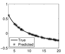
(a) Skewness of Beta

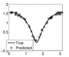
(b) Entropy of Gaussian

Figure 2: (a) Learned skewness of $Beta(a,3)$ distribution. Axis $x$: parameter $a$ in $[3,20]$. Axis $y$: skewness of $Beta(a,3)$. (b) Learned entropy of a 1d marginal distribution of a rotated 2d Gaussian distribution. Axes $x$: rotation angle in $[0,\pi]$. Axis $y$: entropy.

8 Discussion and Conclusion

We have presented an estimator for distribution regression which is distribution-free in the sense that the estimator makes no strong distributional assumptions on the error variables. We derived upper bounds on the risk of the estimator and, in particular, we analyzed the case with a finite doubling dimension.

We note that our rates are faster than the logarithmic rates that are sometimes obtained in measurement error nonparametric regression models as in Fan and Truong (1993). The reason is that the logarithmic rates occur when the measurement error is Gaussian. Our measurement error corresponds to $||\widehat{p}_{i}-p_{i}||$ which is not Gaussian for finite $n_{i}$ and which decreases when $n_{i}$ increases. In the standard measurement error model, the error is $O(1)$ and is not decreasing.

In future work, we will prove lower bounds which show that, without further assumptions (such as assumptions about the doubling dimension), the rates can be very slow. Also, we will show that similar results hold for other estimators such as $k$-nn estimators and RKHS estimators.

Supplementary material

Proof of Lemma 4

Proof. The proof follows the argument of Györfi et al. [2002].

$$\mathbb{P}\Bigl{(}\sum_{i=1}^{m}K_{i}<\underline{K}\Bigr{)} =\mathbb{P}\left(\sum_{i=1}^{m}K\left(\frac{D(P_{i},P)}{h}\right)<\underline{K}\right)$$

$$\leq\mathbb{P}\left(\sum_{i=1}^{m}I_{\{D(P_{i},P)\geq rh\}}=0\right),$$

since according to our assumptions on kernel $K$ if for some $i$ it holds that $D(P_{i},P)/h\leq r$, then $K_{i}\geq$ K. Therefore,

$$\mathbb{P} \Bigl{(}\sum_{i=1}^{m}K_{i}<\underline{K}\Bigr{)}\leq\mathbb{P}\left(\sum_{i=1}^{m}I_{\{D(P_{i},P)\geq rh\}}=0\right)$$

$$=\mbox{$\mathbb{E}$}[\mathbb{P}(\sum_{i=1}^{m}I_{\{D(P_{i},P)\geq rh\}}=0\,|P)]$$

$$=\int\mathbb{P}\left(\sum_{i=1}^{m}I_{\{D(P_{i},P)\geq rh\}}=0\,\bigg{|}P\right)d\mathcal{P}(P)$$

$$=\int[1-\mathcal{P}(P_{1}\in\mathcal{B}(P,rh)|P)]^{m}d\mathcal{P}(P)$$ (15)

$$\leq\int\exp[-m\mathcal{P}(P_{1}\in\mathcal{B}(P,rh)|P)]d\mathcal{P}(P)$$ (16)

$$=\int\exp[-m\mathcal{P}(P_{1}\in\mathcal{B}(P,rh)|P)]$$

$$\qquad\times\frac{m\mathcal{P}(P_{1}\in\mathcal{B}(P,rh)|P)}{m\mathcal{P}(P_{1}\in\mathcal{B}(P,rh)|P)}d\mathcal{P}(P)$$

$$\leq\max_{u>0}u\exp(-u)\int\frac{d\mathcal{P}(P)}{m\mathcal{P}(P_{1}\in\mathcal{B}(P,rh)|P)}$$ (17)

$$\leq\frac{1}{e}\int\frac{d\mathcal{P}(P)}{m\mathcal{P}(P_{1}\in\mathcal{B}(P,rh)|P)}=\frac{1}{em}\mathbb{E}\left[\frac{1}{\Phi_{P}(rh)}\right],$$

where we used in (15), (16), and (17) respectively that $\{P_{i}\}$ are iid, $(1-u)^{m}\leq\exp(-um)$ for all $0\leq u\leq 1$, $m\geq 1$, and $\max(u\exp(-u))=\frac{1}{e}$. $\Box$

Proof of Lemma 5

Proof.

$$\mathbb{E} \left[\frac{1}{\sum_{i}K_{i}}I_{\{\sum_{i}K_{i}\geq\underline{K}\}}\right]\leq\mbox{$\mathbb{E}$}\left[\frac{1+1/\underline{K}}{1+\sum_{i}K_{i}}\right]$$

$$\leq\mbox{$\mathbb{E}$}\left[\frac{1+1/\underline{K}}{1+\underline{K}\sum_{i}I_{\{D(P_{i},P)\leq hR\}}}\right]$$

$$=\frac{1+1/\underline{K}}{\underline{K}}\ \mbox{$\mathbb{E}$}\left[\frac{1}{1/\underline{K}+\sum_{i}I_{\{D(P_{i},P)\leq hR\}}}\right]$$

$$\leq\frac{1+1/\underline{K}}{\underline{K}}\ \mbox{$\mathbb{E}$}\left[\frac{1}{1+\sum_{i}I_{\{D(P_{i},P)\leq hR\}}}\right]$$

$$=\frac{1+1/\underline{K}}{\underline{K}}\ \mbox{$\mathbb{E}$}\bigg{[}\left[\frac{1}{1+\sum_{i}I_{\{D(P_{i},P)\leq hR\}}}\big{|}P\right]\bigg{]}$$

$$\leq\frac{1+1/\underline{K}}{m\underline{K}}\mbox{$\mathbb{E}$}\bigg{[}\frac{1}{\Phi_{P}(Rh)}\bigg{]},$$

where the second-to-last line uses the fact that $\underline{K}<1$ and the last line follows since for a binomial random variable $B(m,p)$, $\mbox{$\mathbb{E}$}[\frac{1}{1+B(m,p)}]\leq\frac{1}{(m+1)p}\leq\frac{1}{mp}$. $\Box$

Proof of Lemma 6

Proof. $D(P,Q)$ is a distance, therefore the triangle inequality holds, and we have that

$$|\epsilon_{i}|=|K_{i}-\widehat{K}_{i}| =\left|K(\frac{D(P,P_{i})}{h})-K(\frac{D(\widehat{P},\widehat{P}_{i})}{h})\right|$$

$$\leq\frac{L_{K}}{h}|{D(P,P_{i})}-{D(\widehat{P},\widehat{P}_{i})}|$$

$$\leq\frac{L_{K}}{h}({D(P,\widehat{P})}+{D(P_{i},\widehat{P}_{i})}).$$

Here we used that

$$D (P,P_{i})-D(\widehat{P},\widehat{P}_{i})$$

$$\leq[D(P,\widehat{P})+D(\widehat{P},\widehat{P}_{i})+D(\widehat{P}_{i},P_{i})]-D(\widehat{P},\widehat{P}_{i})$$

$$=D(P,\widehat{P})+D(\widehat{P}_{i},P_{i}),$$

and

$$D (\widehat{P},\widehat{P}_{i})-D(P,P_{i})$$

$$\leq[D(\widehat{P},P)+D(P,P_{i})+D(P_{i},\widehat{P}_{i})]-D(P,P_{i})$$

$$=D(\widehat{P},P)+D(P_{i},\widehat{P}_{i}).$$

$\Box$

Proof of Lemma 7

Proof. From Markov’s inequality, for any $X$, $Y$ and constant $\kappa>0$,

$$1\leq\frac{\mbox{$\mathbb{E}$}[|X|\,|Y]}{\kappa}+\mathbb{P}(|X|<\kappa|Y).$$

Thus,

$$\mathbb{P} \Bigl{(}\sum_{i}|\epsilon_{i}|<\kappa\Bigm{|}\{P_{i}\}_{i=1}^{m},P\Bigr{)}$$ (18)

$$\geq 1-\frac{\mbox{$\mathbb{E}$}[\sum_{i}|\epsilon_{i}||\{P_{i}\}_{i=1}^{m},P]}{\kappa}$$

$$=1-\frac{\sum_{i}\mbox{$\mathbb{E}$}[|\epsilon_{i}||P_{i},P]}{\kappa}$$

$$\geq 1-\frac{L_{K}}{h\kappa}{\sum_{i=1}^{m}\mbox{$\mathbb{E}$}[({D(P,\widehat{P})}+{D(P_{i},\widehat{P}_{i})})|P_{i},P]}$$ (19)

$$\geq 1-\frac{L_{K}}{h\kappa}{m2\bar{C}n^{-\frac{1}{2+k}}}=\eta(\kappa,n,m).$$

Here (19) holds due to Lemma 6, and we also used (7). $\Box$

Proof of Lemma 8

Proof. The term $\mbox{$\mathbb{E}$}\left[\sum_{i=1}^{m}|\epsilon_{i}|\bigg{|}P,\{P_{i}\}_{i=1}^{m}\right]$ is upper bounded by

$$\frac{L_{K}}{h}\sum_{i=1}^{m}\mbox{$\mathbb{E}$}\left[D(P,\widehat{P})+D(P_{i},\widehat{P}_{i})\bigg{|}P,\{P_{i}\}_{i=1}^{m}\right]$$

$$\leq\frac{L_{K}}{h}2\bar{C}mn^{-\frac{1}{2+k}}.$$

$\Box$

Proof of Lemma 9

Proof. Recall that $D(\widehat{P}_{i},P_{i})\leq rh/4$ for all $i$ on an event $\Omega_{m,n}$ and that $\mathbb{P}(\Omega_{m,n}^{c})\leq(m+1)e^{-\frac{1}{2}n^{\frac{k}{2+k}}}$. So, on $\Omega_{m,n}$,

$$D(\widehat{P}_{i},\widehat{P}) \leq D(\widehat{P}_{i},P_{i})+D(P,\widehat{P})+D(P_{i},P)$$

$$\leq D(P_{i},P)+\frac{rh}{2}.$$

Now, using the event $\Omega_{m,n}$ defined in Lemma 3,

$$\mathbb{P} \Bigl{(}\sum_{i=1}^{m}\widehat{K}_{i}=0\Bigr{)}\leq\mathbb{P}\Bigl{(}\sum_{i=1}^{m}\widehat{K}_{i}<\underline{K}\Bigr{)}$$

$$=\mathbb{P}\Bigl{(}\Omega_{m,n},\sum_{i=1}^{m}\widehat{K}_{i}<\underline{K}\Bigr{)}+\mathbb{P}\Bigl{(}\Omega_{m,n}^{c},\sum_{i=1}^{m}\widehat{K}_{i}<\underline{K}\Bigr{)}$$

$$\leq\mathbb{P}\Bigl{(}\Omega_{m,n},\sum_{i=1}^{m}\widehat{K}_{i}<\underline{K}\Bigr{)}+\mathbb{P}\Bigl{(}\Omega_{m,n}^{c}\Bigr{)}$$

$$\leq\mathbb{P}\Bigl{(}\Omega_{m,n},\sum_{i=1}^{m}\widehat{K}_{i}<\underline{K}\Bigr{)}+(m+1)e^{-\frac{1}{2}n^{\frac{k}{2+k}}}$$

and

$$\mathbb{P}\Bigl{(}\Omega_{m,n},\sum_{i=1}^{m}\widehat{K}_{i}<\underline{K}\Bigr{)} =\mathbb{P}(\Omega_{m,n},\sum_{i=1}^{m}I_{D(\widehat{P}_{i},\widehat{P})\geq rh}=0)$$

$$\leq\mathbb{P}(\sum_{i=1}^{m}I_{D(P_{i},P)\geq rh/2}=0)$$

$$\leq\frac{1}{em}\mathbb{E}\left[\frac{1}{\Phi_{P}(rh/2)}\right].$$

The result follows. $\Box$

Proof of Lemma 10

Proof.

$$\mathbb{E} \left[\Delta\widehat{f}I_{E_{2}}I_{\widehat{E}_{2}}\right]=\mbox{$\mathbb{E}$}\left[\left|\frac{\sum_{i}Y_{i}\widehat{K}_{i}}{\sum_{j}\widehat{K}_{j}}-\frac{\sum_{i}Y_{i}K_{i}}{\sum_{j}K_{j}}\right|I_{E_{2}}I_{\widehat{E}_{2}}\right]$$

$$=\mbox{$\mathbb{E}$}\left[\left|\sum_{i}Y_{i}\left(\frac{K_{i}}{\sum_{j}K_{j}}-\frac{\widehat{K}_{i}}{\sum_{j}\widehat{K}_{j}}\right)\right|I_{E_{2}}I_{\widehat{E}_{2}}\right]$$

$$\leq B_{Y}\mbox{$\mathbb{E}$}\left[\sum_{i}\left|\left(\frac{K_{i}}{\sum_{j}K_{j}}-\frac{\widehat{K}_{i}}{\sum_{j}\widehat{K}_{j}}\right)\right|I_{E_{2}}I_{\widehat{E}_{2}}\right]$$

$$=B_{Y}\mbox{$\mathbb{E}$}\left[\sum_{i}\left(\frac{|K_{i}(\sum_{j}\widehat{K}_{j})-\widehat{K}_{i}(\sum_{j}K_{j})|}{(\sum_{j}\widehat{K}_{j})(\sum_{j}K_{j})}\right)I_{E_{2}}I_{\widehat{E}_{2}}\right]$$

$$=B_{Y}\mbox{$\mathbb{E}$}\bigg{[}\sum_{i}\left(\frac{|(\widehat{K}_{i}-\epsilon_{i})(\sum_{j}\widehat{K}_{j})-\widehat{K}_{i}(\sum_{j}(\widehat{K}_{j}-\epsilon_{j}))|}{(\sum_{j}\widehat{K}_{j})(\sum_{j}K_{j})}\right)$$

$$\qquad\qquad\times I_{E_{2}}I_{\widehat{E}_{2}}\bigg{]}$$

$$=B_{Y}\mbox{$\mathbb{E}$}\bigg{[}\sum_{i}\left(\frac{|-\epsilon_{i}(\sum_{j}\widehat{K}_{j})+\widehat{K}_{i}(\sum_{j}\epsilon_{j})|}{(\sum_{j}\widehat{K}_{j})(\sum_{j}K_{j})}\right)I_{E_{2}}I_{\widehat{E}_{2}}\bigg{]}$$

$$\leq B_{Y}\mbox{$\mathbb{E}$}\bigg{[}\bigg{(}\frac{(\sum_{i}\widehat{K}_{i})(\sum_{j}|\epsilon_{j}|)}{(\sum_{j}\widehat{K}_{j})(\sum_{j}K_{j})}$$

$$\quad+\frac{(\sum_{i}|\epsilon_{i}|)(\sum_{j}\widehat{K}_{j})}{(\sum_{j}\widehat{K}_{j})(\sum_{j}K_{j})}\bigg{)}I_{E_{2}}I_{\widehat{E}_{2}}\bigg{]}$$

$$=B_{Y}\mbox{$\mathbb{E}$}\bigg{[}\bigg{(}\frac{\sum_{j}|\epsilon_{j}|}{\sum_{j}K_{j}}+\frac{(\sum_{i}|\epsilon_{i}|)}{\sum_{j}K_{j}}\bigg{)}I_{E_{2}}I_{\widehat{E}_{2}}\bigg{]}$$

$$\leq 2B_{Y}\mbox{$\mathbb{E}$}\bigg{[}\frac{\sum_{j}|\epsilon_{j}|}{\sum_{j}K_{j}}I_{E_{2}}\bigg{]}$$

$$=\mbox{$\mathbb{E}$}\bigg{[}\mbox{$\mathbb{E}$}\bigg{[}\sum_{j}|\epsilon_{j}||P,\{P_{i}\}_{i=1}^{m}\bigg{]}\frac{1}{\sum_{j}K_{j}}I_{E_{2}}\bigg{]}$$

$$\leq 2B_{Y}\frac{L_{K}}{h}2\widehat{c}mn^{-\frac{1}{2+k}}\mbox{$\mathbb{E}$}\bigg{[}\frac{1}{\sum_{j}K_{j}}I_{E_{2}}\bigg{]}$$

$$\leq 2B_{Y}\frac{L_{K}}{h}2\widehat{c}mn^{-\frac{1}{2+k}}\frac{1+1/\underline{K}}{m\underline{K}}\mbox{$\mathbb{E}$}\left[\frac{1}{\Phi_{P}(Rh)}\right]$$

$$=C_{1}\frac{1}{h}\mbox{$\mathbb{E}$}\bigg{[}\frac{1}{\Phi_{P}(Rh)}\bigg{]}n^{-\frac{1}{2+k}}.$$

where we used Lemma 8 and Lemma 5. $\Box$

Proof of Theorem 11

Proof.

$$\mbox{$\mathbb{E}$}|\widehat{f} (\widehat{P};\widehat{P}_{1},\ldots,\widehat{P}_{m})-\widehat{f}(P;P_{1},\ldots,P_{m})|$$

$$\leq\mbox{$\mathbb{E}$}\left[\Delta\widehat{f}I_{E_{2}}I_{\widehat{E}_{2}}\right]+3B_{Y}\zeta+3\frac{B_{Y}}{em}\mbox{$\mathbb{E}$}\bigg{[}\frac{1}{\Phi_{P}(rh)}\bigg{]}$$

$$\leq C_{1}\frac{1}{h}\mbox{$\mathbb{E}$}\bigg{[}\frac{1}{\Phi_{P}(Rh)}\bigg{]}n^{-\frac{1}{2+k}}+C_{2}\frac{1}{m}\mathbb{E}\left[\frac{1}{\Phi_{P}(rh)}\right]$$

$$\qquad+C_{3}\frac{1}{m}\mathbb{E}\left[\frac{1}{\Phi_{P}(rh/2)}\right]+(m+1)e^{-\frac{1}{2}n^{\frac{k}{2+k}}}.$$

Note also that $\Phi_{P}(rh/2)\leq\Phi_{P}(rh)\leq\Phi_{P}(Rh)$. $\Box$

Proof of Lemma 12

Proof. Notice that if $\sum_{i}K_{i}\geq\underline{K}>0$,

$$\text{var}\left(\frac{\sum_{i}\mu_{i}K_{i}}{\sum_{i}K_{i}}|P,P_{1},\dots,P_{m}\right)\leq B_{Y}^{2}\frac{\sum_{i}K_{i}^{2}}{(\sum_{i}K_{i})^{2}}.$$

Using this and Hölder’s inequality, we get:

$$\mbox{$\mathbb{E}$}\left[\left|\frac{\sum_{i}\mu_{i}K_{i}}{\sum_{i}K_{i}}\right|I_{\{\sum_{i}K_{i}\geq\underline{K}\}}\right]$$

$$=\mbox{$\mathbb{E}$}\left[\mbox{$\mathbb{E}$}\left[\left|\frac{\sum_{i}\mu_{i}K_{i}}{\sum_{i}K_{i}}\right|I_{\sum_{i}K_{i}\geq\underline{K}}|P,P_{1},\dots,P_{m}\right]\right]$$

$$\leq\mbox{$\mathbb{E}$}\left[\sqrt{\text{var}\left(\frac{\sum_{i}\mu_{i}K_{i}}{\sum_{i}K_{i}}|P,P_{1},\dots,P_{m}\right)}I_{\{\sum_{i}K_{i}\geq\underline{K}\}}\right]$$

$$\leq\mbox{$\mathbb{E}$}\left[B_{Y}\frac{\sqrt{\sum_{i}K_{i}^{2}}}{\sum_{i}K_{i}}I_{\{\sum_{i}K_{i}\geq\underline{K}\}}\right]$$

$$\leq\mbox{$\mathbb{E}$}\left[B_{Y}\frac{\sqrt{\sum_{i}K_{i}}}{\sum_{i}K_{i}}I_{\{\sum_{i}K_{i}\geq\underline{K}\}}\right]$$

$$\leq B_{Y}\sqrt{\mbox{$\mathbb{E}$}\left[\frac{\sum_{i}K_{i}}{(\sum_{i}K_{i})^{2}}I_{\{\sum_{i}K_{i}\geq\underline{K}\}}\right]}$$

$$\leq B_{Y}\sqrt{\mbox{$\mathbb{E}$}\left[\frac{I_{\{\sum_{i}K_{i}\geq\underline{K}\}}}{\sum_{i}K_{i}}\right]}$$

$$\leq B_{Y}\sqrt{\frac{1+1/\underline{K}}{m\underline{K}}\ \int\frac{d\mathcal{P}(P)}{\Phi_{P}(Rh)}}.$$

The second inequality holds since $K(x)<1$ and the last step stems from Lemma 5. $\Box$

References

Carroll et al. (2006)
R.J. Carroll, D. Ruppert, L.A. Stefanski, and C.M. Crainiceanu.
Measurement error in nonlinear models: a modern perspective,
volume 105.
Chapman & Hall/CRC, 2006.
Christmann and Steinwart (2010)
A. Christmann and I. Steinwart.
Universal kernels on non-standard input spaces.
In NIPS, pages 406–414, 2010.
Devroye and Lugosi (2001)
L. Devroye and G. Lugosi.
Combinatorial methods in density estimation.
Springer, 2001.
Fan and Truong (1993)
J. Fan and Y.K. Truong.
Nonparametric regression with errors in variables.
The Annals of Statistics, pages 1900–1925, 1993.
Ferraty and Vieu (2006)
F. Ferraty and P. Vieu.
Nonparametric Functional Data Analysis: Theory and Practice.
Springer Verlag, 2006.
Györfi et al. (2002)
L. Györfi, M. Kohler, A. Krzyzak, and H. Walk.
A Distribution-Free Theory of Nonparametric Regression.
Springer, New-york, 2002.
Jaakkola and Haussler (1998)
T. Jaakkola and D. Haussler.
Exploiting generative models in discriminative classifiers.
In NIPS, pages 487–493. MIT Press, 1998.
Jebara et al. (2004)
T. Jebara, R. Kondor, A. Howard, K. Bennett, and N. Cesa-bianchi.
Probability product kernels.
JMLR, 5:819–844, 2004.
Kondor and Jebara (2003)
R. Kondor and T. Jebara.
A kernel between sets of vectors.
In ICML, 2003.
Kpotufe (2011)
S. Kpotufe.
k-nn regression adapts to local intrinsic dimension.
arXiv preprint arXiv:1110.4300, 2011.
Moreno et al. (2004)
P. Moreno, P. Ho, and N. Vasconcelos.
A Kullback-Leibler divergence based kernel for SVM
classification in multimedia applications.
In NIPS, 2004.
Muandet et al. (2012)
K. Muandet, B. Schölkopf, K. Fukumizu, and F. Dinuzzo.
Learning from distributions via support measure machines.
arXiv.org, stat.ML, February 2012.
Póczos et al. (2011)
B. Póczos, L. Xiong, and J. Schneider.
Nonparametric divergence estimation with applications to machine
learning on distributions.
In UAI, 2011.
Póczos et al. (2012)
B. Póczos, L. Xiong, D. Sutherland, and J. Schneider.
Nonparametric kernel estimators for image classification.
In Computer Vision and Pattern Recognition, 2012.
Ramsay and Silverman (2005)
J.O. Ramsay and B.W Silverman.
Functional data analysis.
Springer, New York, 2nd edition, 2005.
Rigollet and Vert (2009)
P. Rigollet and R. Vert.
Optimal rates for plug-in estimators of density level sets.
Bernoulli, 15(4):1154–1178, 2009.
Smola et al. (2007)
A. Smola, A. Gretton, L. Song, and B. Schölkopf.
A Hilbert space embedding for distributions.
In ALT, 2007.
Tsybakov (2010)
A.B. Tsybakov.
Introduction to Nonparametric Estimation.
Springer, 2010.