Precise QCD predictions on $W_{H}Z_{H}$ production in the littlest Higgs Model with $T$ parity at the LHC

Abstract

We investigate the effects of the littlest Higgs model with $T$ parity up to the QCD next-to-leading order (NLO) on the $W_{H}^{\pm}Z_{H}$ productions at the CERN Large Hadron Collider (LHC), and discuss the kinematic distributions of final decay products and the theoretical dependence of the cross section on the factorization/renormalization scale. We find the QCD NLO corrections reduce the scale uncertainty of the leading order cross section in case of $\mu_{F}=\mu_{R}$. By adopting the PROSPINO subtraction scheme (scheme (II)) in analysing the QCD NLO contributions, we can obtain the numerical results which keep the convergence of the perturbative QCD description. Our results by adopting scheme (II) at the $14~{}{\rm TeV}$ ($8~{}{\rm TeV}$) LHC show that the $K$-factor for the $W_{H}^{+}Z_{H}$ production varies in the range of $1.01\sim 1.10$ ($1.00\sim 1.08$), while the $K$-factor for the $W_{H}^{-}Z_{H}$ production varies in the range of $1.11\sim 1.13$ ($1.11\sim 1.12$), when the global symmetry breaking scale $f$ goes from $400~{}{\rm GeV}$ to $1.5~{}{\rm TeV}$ ($1~{}{\rm TeV}$).

PACS: 12.38.Bx, 12.60.Cn, 14.70.Pw

I. Introduction

To interpret the mechanism of electroweak symmetry breaking and resolve the little hierarchy problem [1] are the major motivations for the little Higgs models [2]. In those models some new gauge bosons, scalars and fermions are introduced at a global symmetry breaking scale $f$ to cancel the one-loop quadratic divergences for the Higgs mass from the standard model (SM) [3, 4] particles. It deserves much attention due to their elegant solution to the hierarchy problem and they are proposed as one kind of electroweak symmetry breaking models without fine-tuning. Among the little Higgs models there is one simplest version, the littlest Higgs (LH) model, providing a set of new heavy gauge bosons ($W_{H},Z_{H},A_{H}$) and a vector-like quark ($T$) to implement the divergence cancellation. Nevertheless, precision electroweak measurements [5] severely constrain the LH model, especially the recent experimental measurements [6, 7] on the searching for $W_{H}$ and $Z_{H}$ bosons.

The precision electroweak constraints require the LH model characterize a large value of $f$. To avoid fine-tuning between the global symmetry breaking scale $f$ and the electroweak symmetry breaking scale, a discrete symmetry named $T$ parity [8]-[10] is imposed. In this way, the heavy gauge bosons assigned to be $T$-odd particles do not directly couple with a pair of SM fermions and all dangerous tree-level contributions to the precision measurements are forbidden, therefore, the phenomenological constraints are somewhat relaxed. Thus the LH model with $T$ parity (LHT) [8]-[12] deserves more attention. In the LHT, heavy gauge bosons, heavy fermions and heavy leptons acquire masses through the breaking of the global symmetry, and there exists an attractive dark matter candidate $A_{H}$ [13]. The global symmetry breaking scale $f$ can be lower than $1~{}{\rm TeV}$ [10], and the processes $W_{H}^{\mp}\to l^{\mp}\stackrel{{\scriptstyle(-)}}{{\nu}}$ and $Z_{H}\to l^{+}l^{-}$ are forbidden due to the $T$ parity conservation, leaving the only $T$-odd heavy gauge boson decay modes $W_{H}^{\pm}\to A_{H}W^{\pm}$ and $Z_{H}\to A_{H}H$, where $H$ is the lightest neutral Higgs boson, followed by the subsequential leptonic decays of $W^{\pm}$ and Higgs boson. As a result, the experimental constraints [6, 7] on $m_{W_{H}}$ and $m_{Z_{H}}$ can not be applied to the $T$-odd gauge bosons in the LHT. Recently, some QCD NLO phenomenological aspects of the LHT have been analyzed in Refs.[14, 15]. The $W_{H}Z_{H}$ production at the LHC can be significant in searching for the new gauge bosons due to the potential of its copious productions as shown in Refs.[16, 17], where the $W_{H}Z_{H}$ production at the LHC is only studied at the leading-order (LO).

The purpose of this work is to perform a comprehensive analysis for the processes $pp\to W_{H}^{\pm}Z_{H}+X~{}$at the LHC up to the QCD NLO. In Sec.II a brief review of the related LHT theory is given. In Sec.III we present the details of the calculations. The numerical results and discussions are provided in Sec.IV. Finally we give a short summary.

II. Related LHT theory

In order to fix notations used in this paper we briefly review the relevant LHT theory. The details of the LHT theory can be found in Refs.[8, 9, 10, 16].

In the LHT the assumed global symmetry $SU(5)$ is broken down spontaneously to $SO(5)$ at some high scale $f$ around $1~{}{\rm TeV}$ [18]. Breaking of $SU(5)$ leads to 14 massless Nambu-Goldstone bosons, which transform under the electroweak gauge group, $SU(2)_{L}\times U(1)_{Y}$, as a real singlet, a real triplet, a complex doublet and a complex triplet. Four of the Nambu-Goldstone bosons are treated as longitudinal components of the heavy gauge bosons. The others decompose into a $T$-even $SU(2)$ doublet $h$, identified as the SM Higgs doublet, and a complex $T$-odd $SU(2)$ triplet $\Phi$.

The $T$ parity transformations for the gauge sector are defined as the exchange between the gauge bosons of the two $SU(2)\times U(1)$ groups, i.e., $W_{1}^{a}\leftrightarrow W_{2}^{a}$ and $B_{1}\leftrightarrow B_{2}$. The gauge couplings of the two gauge groups have to be equal, i.e., $g_{1}=g_{2}=\sqrt{2}g$ and $g^{\prime}_{1}=g^{\prime}_{2}=\sqrt{2}g^{\prime}$. Thus their $T$-odd and $T$-even combinations can be obtained as

$$W_{H}^{a}=\frac{1}{\sqrt{2}}(W_{1}^{a}-W_{2}^{a}), B_{H}=\frac{1}{\sqrt{2}}(B_{1}-B_{2}), (T-{\rm odd}),$$

$$W_{L}^{a}=\frac{1}{\sqrt{2}}(W_{1}^{a}+W_{2}^{a}), B_{L}=\frac{1}{\sqrt{2}}(B_{1}+B_{2}), (T-{\rm even}).$$ (2.1)

The mass eigenstates of the gauge sector in the LHT are expressed as

$$W_{H}^{\pm}=\frac{1}{\sqrt{2}}(W_{H}^{1}\mp iW_{H}^{2}), Z_{H}=\sin{\theta_{H}}B_{H}+\cos{\theta_{H}}W^{3}_{H}, A_{H}=\cos{\theta_{H}}B_{H}-\sin{\theta_{H}}W^{3}_{H},$$

$$W_{L}^{\pm}=\frac{1}{\sqrt{2}}(W_{L}^{1}\mp iW_{L}^{2}), Z_{L}=-\sin{\theta_{W}}B_{L}+\cos{\theta_{W}}W^{3}_{L}, A_{L}=\cos{\theta_{W}}B_{L}+\sin{\theta_{W}}W^{3}_{L},$$ (2.2)

where $\theta_{W}$ is the Weinberg angle, and the mixing angle $\theta_{H}$ at the ${\cal O}(v_{SM}^{2}/f^{2})$ is expressed as

$$\sin\theta_{H}\simeq\left[\frac{5gg^{\prime}}{4(5g^{2}-g^{\prime 2})}\frac{v_{SM}^{2}}{f^{2}}\right].$$ (2.3)

The $T$-even gauge bosons $A_{L}$, $Z_{L}$ and $W_{L}^{\pm}$ are identified with the SM gauge bosons, while the four new heavy gauge bosons, the $T$-odd partners of SM gauge bosons, are $A_{H}$, $Z_{H}$ and $W_{H}^{\pm}$ with masses of [16]

$$m_{A_{H}}\simeq\frac{1}{\sqrt{5}}g^{\prime}f\left(1-\frac{5}{8}\frac{v_{SM}^{2}}{f^{2}}\right), m_{Z_{H}}\simeq m_{W_{H}}\simeq gf\left(1-\frac{1}{8}\frac{v_{SM}^{2}}{f^{2}}\right),$$ (2.4)

where $v_{SM}=246~{}{\rm GeV}$. The $T$ parity partner of photon, $A_{H}$, is the lightest $T$-odd particle. Therefore, the heavy photon is a candidate of dark matter. The masses of SM gauge bosons can be expressed as $m_{W}=\frac{1}{2}gv_{SM}$ and $m_{Z}=\frac{1}{2}\sqrt{g^{2}+g^{\prime 2}}v_{SM}$ at the tree-level.

When the $T$ parity is implemented in the fermion sector of the model, the existence of mirror partners for each of the original fermions are required. The $T$-odd partners of SM up- and down-type quarks are denoted as $U_{-}$ and $D_{-}$, where $U_{-}=u_{-},c_{-},t_{-}$ and $D_{-}=d_{-},s_{-},b_{-}$. We can get their masses as [16]

$$m_{U_{-}}\simeq\sqrt{2}\kappa f\left(1-\frac{1}{8}\frac{v_{SM}^{2}}{f^{2}}\right), m_{D_{-}}=\sqrt{2}\kappa f,$$ (2.5)

where $\kappa$ is the mass coefficient in Lagrangian of the quark sector. The Feynman rules in the LHT used in this work are presented in Appendix.

III. Calculations

In the LO and QCD NLO calculations we employ the FeynArts 3.4 package [19] to generate Feynman diagrams and their corresponding amplitudes. To implement the amplitude calculations we apply FormCalc 5.4 programs [20]. The t’Hooft-Feynman gauge and the five-flavor scheme (5FS) are adopted in this work.

III..1 LO cross section

At the parton level the cross section for the $qq^{\prime}\to W_{H}^{-}Z_{H}$ $(qq^{\prime}=\bar{u}d,\bar{u}s,\bar{c}d,\bar{c}s)$ subprocess in the LHT should be the same as that for the corresponding charge conjugate subprocess $qq^{\prime}\to W_{H}^{+}Z_{H}$ $(qq^{\prime}=u\bar{d},u\bar{s},c\bar{d},c\bar{s})$ due to the $CP$-conservation. We present the parton level calculations for the related subprocess $qq^{\prime}\to W_{H}^{+}Z_{H}$ in this section. By neglecting the contribution of bottom quark in the initial state, the LO contribution to the cross section for the parent process $pp\to W_{H}^{+}Z_{H}+X$ comes from the subprocesses

$$q(p_{1})+q^{\prime}(p_{2})\to W_{H}^{+}(p_{3})+Z_{H}(p_{4}), (qq^{\prime}=u\bar{d},u\bar{s},c\bar{d},c\bar{s}),$$ (3.1)

where $p_{i}~{}(i=1,2,3,4)$ represent the four-momenta of the incoming partons and the outgoing $W_{H}^{+}$, $Z_{H}$ bosons, respectively. The Feynman diagrams for the $u\bar{d}\to W_{H}^{+}Z_{H}$ partonic process are shown in Fig.1, and the LO Feynman graphs for other relevant partonic processes $qq^{\prime}\to W_{H}^{+}Z_{H}$ ($qq^{\prime}=u\bar{s},c\bar{d},c\bar{s}$) are similar with those in Fig.1.

The expression for the LO cross section for the partonic process $qq^{\prime}\to W_{H}^{+}Z_{H}$ ($qq^{\prime}=u\bar{d},u\bar{s},c\bar{d},c\bar{s}$) has the form as

$$\hat{\sigma}^{0}_{qq^{\prime}}=\frac{1}{4}\frac{1}{9}\frac{1}{4|\vec{p}|\sqrt{\hat{s}}}\int\sum_{spin}\sum_{color}|{\cal M}^{LO}_{qq^{\prime}}|^{2}d\Omega_{2}, (qq^{\prime}=u\bar{d},u\bar{s},c\bar{d},c\bar{s}),$$ (3.2)

where the factors $\frac{1}{4}$ and $\frac{1}{9}$ come from averaging over the spins and colors of the initial partons, respectively, $\vec{p}$ is the three-momentum of one initial parton in center-of-mass system, $\sqrt{\hat{s}}$ is the partonic center-of-mass system energy and ${\cal M}_{qq^{\prime}}^{LO}$ is the amplitude of all the tree-level diagrams for the partonic process $qq^{\prime}\to W_{H}^{+}Z_{H}$. The summation is taken over the spins and colors of all the relevant particles in the $qq^{\prime}\to W_{H}^{+}Z_{H}$ subprocess. We perform the integration over the two-body phase space of the final particles $W_{H}^{+}$ and $Z_{H}$. The phase space element $d\Omega_{2}$ is expressed as

$$d\Omega_{2}=(2\pi)^{4}\delta^{(4)}(p_{1}+p_{2}-p_{3}-p_{4})\frac{d^{3}\vec{p}_{3}}{(2\pi)^{3}2E_{3}}\frac{d^{3}\vec{p}_{4}}{(2\pi)^{3}2E_{4}}.$$ (3.3)

Figure 1: The LO Feynman diagrams for the partonic process $u\bar{d}\to W_{H}^{+}Z_{H}~{}$.

Then the LO total cross section for the parent process $pp\to W_{H}^{+}Z_{H}+X$ can be expressed as

$$\sigma_{LO}=\sum_{qq^{\prime}=u\bar{d},u\bar{s},}^{c\bar{d},c\bar{s}}\int_{0}^{1}dx_{1}\int_{0}^{1}dx_{2}\left[G_{q/P_{1}}(x_{1},\mu_{F})G_{q^{\prime}/P_{2}}(x_{2},\mu_{F})+(1\leftrightarrow 2)\right]\hat{\sigma}^{0}_{qq^{\prime}}(\hat{s}=x_{1}x_{2}s),$$ (3.4)

where $G_{j/P}$ $(j=u,c,\bar{d},\bar{s})$ is the parton distribution function (PDF) of proton $P$, which describes the probability in finding a parton $j$ with momentum $xp_{j}$ in proton $P$, $s$ represents the total colliding energy squared in the rest frame of proton-proton system, and $\mu_{F}$ is the factorization scale.

III..2 QCD NLO corrections

The QCD NLO corrections to the parent process $pp\to W_{H}^{+}Z_{H}+X$ at the LHC can be divided into four parts:

• The QCD one-loop virtual corrections to the partonic processes $qq^{\prime}\to W_{H}^{+}Z_{H}$;

• The contributions of the real gluon emission partonic processes $qq^{\prime}\to W_{H}^{+}Z_{H}+g$;

• The contributions of the real light-(anti)quark emission partonic processes $qg\to W_{H}^{+}Z_{H}+q^{\prime}$;

• The contributions of the PDF counterterms.

The dimensional regularization method in $D=4-2\epsilon$ dimensions is adopted in this work to isolate the ultraviolet (UV) and infrared (IR) singularities in the NLO calculations.

III..2.1 One-loop virtual corrections to $qq^{\prime}\to W_{H}^{+}Z_{H}~{}$partonic process

Some representative Feynman diagrams for the one-loop virtual corrections to the partonic process $u\bar{d}\to W_{H}^{+}Z_{H}~{}$are presented in Fig.2. There exist both UV and IR singularities. The masses and wave functions of SM quarks and their $T$-odd partners should be renormalized to remove the UV divergences. The counterterms are defined as

$$\psi^{0,L,R}_{q} = \left(1+\frac{1}{2}\delta Z_{q}^{L,R}\right)\psi^{L,R}_{q}~{},$$ (3.5)

$$\psi^{0,L,R}_{q_{-}} = \left(1+\frac{1}{2}\delta Z_{q_{-}}^{L,R}\right)\psi^{L,R}_{q_{-}}~{},$$ (3.6)

$$m^{0}_{q_{-}} = m_{q_{-}}+\delta m_{q_{-}}~{},$$ (3.7)

where $\psi^{L,R}_{q},\psi^{L,R}_{q_{-}}$ denote the fields of SM quark and $T$-odd quark, respectively, and $m_{q_{-}}$denotes the mass of $T$-odd quark. The on-shell scheme is applied to renormalize the relevant fields and masses, then we obtain

$$\delta Z^{L,R}_{q} = -\frac{\alpha_{s}(\mu_{R})}{3\pi}\left[\Delta_{UV}-\Delta_{IR}\right]~{},$$ (3.8)

$$\delta Z^{L,R}_{q_{-}} = -\frac{\alpha_{s}(\mu_{R})}{3\pi}\left[\Delta_{UV}+2\Delta_{IR}+4+3\ln\left(\frac{\mu_{R}^{2}}{m_{q_{-}}^{2}}\right)\right]~{},$$ (3.9)

$$\frac{\delta m_{q_{-}}}{m_{q_{-}}} = -\frac{\alpha_{s}(\mu_{R})}{3\pi}\left\{3\left[\Delta_{UV}+\ln\left(\frac{\mu_{R}^{2}}{m_{q_{-}}^{2}}\right)\right]+4\right\}~{},$$ (3.10)

where $\Delta_{UV}=\frac{1}{\epsilon_{UV}}-\gamma_{E}+\ln(4\pi)$ and $\Delta_{IR}=\frac{1}{\epsilon_{IR}}-\gamma_{E}+\ln(4\pi)$. The one-loop virtual contribution is UV finite after performing the renormalization procedure. Nevertheless, there still exist soft and collinear IR singularities. By adding the contributions of the real gluon/light-(anti)quark emission subprocesses and the counterterms of the PDFs at the NLO, the remaining singularities are canceled as we shall see later.

Figure 2: The representative one-loop Feynman diagrams for the partonic process $u\bar{d}\to W_{H}^{+}Z_{H}~{}$.

III..2.2 Real gluon/light-(anti)quark emission corrections

The real gluon emission partonic processes for the $W_{H}^{+}Z_{H}$ production can be denoted as

$$q(p_{1})+q^{\prime}(p_{2})\to W_{H}^{+}(p_{3})+Z_{H}(p_{4})+g(p_{5}), (qq^{\prime}=u\bar{d},u\bar{s},c\bar{d},c\bar{s}).$$ (3.11)

The real gluon emission subprocess $qq^{\prime}\to W_{H}^{+}Z_{H}g$ contains both soft and collinear IR singularities which can be conveniently isolated by adopting the two cutoff phase space slicing (TCPSS) method [21]. In Fig.3 we show the tree level Feynman diagrams for this subprocess. In performing the calculations with the TCPSS method, we should introduce two arbitrary small soft cutoff $\delta_{s}$ and collinear cutoff $\delta_{c}$. The phase space of the $qq^{\prime}\to W_{H}^{+}Z_{H}g$ subprocess can be split into two regions: soft gluon region ($E_{5}\leq\frac{1}{2}\delta_{s}\sqrt{\hat{s}}$) and hard gluon region ($E_{5}>\frac{1}{2}\delta_{s}\sqrt{\hat{s}}$) by the soft cutoff $\delta_{s}$. The hard gluon region is separated as hard collinear ($HC$) and hard noncollinear ($\overline{HC}$) regions by the collinear cutoff $\delta_{c}$. The $HC$ region is the phase space where $\hat{s}_{15}\leq\delta_{c}\hat{s}$ or $\hat{s}_{25}\leq\delta_{c}\hat{s}$ ($\hat{s}_{ij}=(p_{i}+p_{j})^{2}$). Then the cross section for the real gluon emission subprocess is written as

$$\hat{\sigma}^{R}_{g}=\hat{\sigma}^{S}_{g}+\hat{\sigma}^{H}_{g}=\hat{\sigma}^{S}_{g}+\hat{\sigma}^{\rm HC}_{g}+\hat{\sigma}^{\overline{\rm HC}}_{g}.$$ (3.12)

According to the Kinoshita-Lee-Nauenberg (KLN) theorem [22], the soft singularity in the soft part $\hat{\sigma}_{g}^{S}$ can be canceled by the soft IR divergence in the virtual corrections, while the hard noncollinear cross section part $\hat{\sigma}_{g}^{\overline{HC}}$ is IR safe. The virtual corrections cancel part of the collinear singularity and the PDF counterterms absorb the remaining collinear divergence.

Beside the real gluon emission subprocesses, the real light-(anti)quark emission subprocesses, which have the same order contributions with the real gluon emission subprocesses, should be taken into account. This kind of subprocesses is denoted as

$$q(p_{1})+g(p_{2})\to W_{H}^{+}(p_{3})+Z_{H}(p_{4})+q^{\prime}(p_{5}), (qq^{\prime}=ud,cs,\bar{d}\bar{u},\bar{s}\bar{c}).$$ (3.13)

The corresponding Feynman diagrams for the subprocess $qg\to W_{H}^{+}Z_{H}+q^{\prime}$ at the tree-level are shown in Fig.4. Using the TCPSS method described above, the phase space can be split into a collinear ($C$) region ($\hat{s}_{15}\leq\delta_{c}\hat{s}$ or $\hat{s}_{25}\leq\delta_{c}\hat{s}$) and a noncollinear ($\overline{C}$) region ($\hat{s}_{15}>\delta_{c}\hat{s}$ and $\hat{s}_{25}>\delta_{c}\hat{s}$) by a collinear cutoff $\delta_{c}$. Therefore, the cross section for the real light-(anti)quark emission subprocess can be expressed as

$$\hat{\sigma}^{R}_{q}=\hat{\sigma}_{q}^{C}+\hat{\sigma}_{q}^{\overline{C}}.$$ (3.14)

The cross section $\hat{\sigma}_{q}^{\overline{C}}$ in the noncollinear region is finite and can be evaluated in four dimensions using Monte Carlo technique while $\hat{\sigma}_{q}^{C}$ contains collinear singularity. After adding the renormalized virtual corrections and the real gluon/light-(anti)quark emission corrections to the subprocess $qq^{\prime}\to W_{H}^{+}Z_{H}~{}$, the partonic cross section still contains the collinear divergence, which can be absorbed into the redefinition of the PDFs at the NLO.

Figure 3: The tree-level Feynman diagrams for the real gluon emission partonic process $qq^{\prime}\to W_{H}^{+}Z_{H}+g$, $(qq^{\prime}=u\bar{d},u\bar{s},c\bar{d},c\bar{s})$.

III..2.3 PDF counterterms

The PDF counterterms, $\delta G_{i/P}(x,\mu_{F})$ ($i=g,u,\bar{u},d,\bar{d},c,\bar{c},s,\bar{s}$), which absorb the remaining collinear divergence, can be split into two parts: the collinear gluon emission part $\delta G_{i/P}^{(gluon)}(x,\mu_{F})$ and the collinear light-quark emission part $\delta G_{i/P}^{(quark)}(x,\mu_{F})$:

$$\delta G_{q(g)/P}(x,\mu_{F})=\delta G_{q(g)/P}^{(gluon)}(x,\mu_{F})+\delta G_{q(g)/P}^{(quark)}(x,\mu_{F}),~{}~{}~{}(q=u,\bar{u},d,\bar{d},c,\bar{c},s,\bar{s}),$$ (3.15)

where

$$\delta G_{q(g)/P}^{(gluon)}(x,\mu_{F})=\frac{1}{\epsilon}\left[\frac{\alpha_{s}}{2\pi}\frac{\Gamma(1-\epsilon)}{\Gamma(1-2\epsilon)}\left(\frac{4\pi\mu_{R}^{2}}{\mu_{F}^{2}}\right)^{\epsilon}\right]\int_{x}^{1}\frac{dz}{z}P_{qq(gg)}(z)G_{q(g)/P}(x/z,\mu_{F}),$$

$$\delta G_{q/P}^{(quark)}(x,\mu_{F})=\frac{1}{\epsilon}\left[\frac{\alpha_{s}}{2\pi}\frac{\Gamma(1-\epsilon)}{\Gamma(1-2\epsilon)}\left(\frac{4\pi\mu_{R}^{2}}{\mu_{F}^{2}}\right)^{\epsilon}\right]\int_{x}^{1}\frac{dz}{z}P_{qg}(z)G_{g/P}(x/z,\mu_{F}),$$

$$\delta G_{g/P}^{(quark)}(x,\mu_{F})=\frac{1}{\epsilon}\left[\frac{\alpha_{s}}{2\pi}\frac{\Gamma(1-\epsilon)}{\Gamma(1-2\epsilon)}\left(\frac{4\pi\mu_{R}^{2}}{\mu_{F}^{2}}\right)^{\epsilon}\right]\sum_{q=u,\bar{u},d,\bar{d},}^{c,\bar{c},s,\bar{s},b,\bar{b},}\int_{x}^{1}\frac{dz}{z}P_{gq}(z)G_{q/P}(x/z,\mu_{F}).~{}~{}~{}$$ (3.16)

More details about the explicit expressions for the splitting functions $P_{ij}(z)(ij=qq,qg,gq,gg)$ are available in Ref.[21].

Figure 4: The tree-level Feynman diagrams for the real light-quark emission partonic process $qg\to W_{H}^{+}Z_{H}+q^{\prime}$ $(qq^{\prime}=ud,cs,\bar{d}\bar{u},\bar{s}\bar{c})$.

III..2.4 Total QCD NLO correction

Finally, we have eliminated all the UV and IR singularities by performing the renormalization procedure and adding all the QCD NLO correction components, and we get the finite QCD NLO corrected integrated cross section for the $pp\to W_{H}^{+}Z_{H}+X$ process as

$$\sigma_{NLO} = \sigma_{LO}+\Delta\sigma_{NLO}=\sigma_{LO}+\Delta\sigma^{(2)}+\Delta\sigma^{(3)}.$$ (3.17)

The two-body term $\Delta\sigma^{(2)}$ includes the one-loop corrections to the $pp\to W_{H}^{+}Z_{H}+X$ process and the tree-level contributions in the soft and hard collinear regions for the real gluon/light-(anti)quark emission processes, while the three-body term $\Delta\sigma^{(3)}$ contains the cross sections for the real gluon/light-(anti)quark emission processes over the hard noncollinear region.

In this work, two event selection schemes are applied in discussing the QCD NLO corrections. In scheme (I) all the NLO correction components mentioned above are included in the QCD NLO corrections, called also the inclusive event selection scheme. In this scheme, there exists resonance effect in Figs.4 (5)-(8) duo to the possible on-shell $q_{-}$ propagator and those Feynman diagrams could lead to large corrections to the Born $pp\to W_{H}^{+}Z_{H}+X$ process, so that the perturbative convergence would be eventually destroyed. To deal with the resonance effect in these partonic processes, the $q_{-}$ mass squared $m_{q_{-}}^{2}$ in its propagator should be replaced by $m_{q_{-}}^{2}-im_{q_{-}}\Gamma_{q_{-}}$. The partial decay widths of $T$-odd quarks are obtained numerically by adopting the expressions presented in Ref.[15].

Actually, the contributions from the diagrams for the $qg\to W_{H}^{+}Z_{H}+q^{\prime}$ subprocess with intermediate on-shell $T$-odd quark $q_{-}$ shown in Figs.4 (5)-(8), should pertain to other on-shell $W_{H}q_{-}$ and $Z_{H}q_{-}$ associated production channels, i.e., $pp\to qg\to W_{H}q_{-}^{\prime}+X$ and $pp\to qg\to Z_{H}q_{-}+X$ processes, followed with subsequential decays of $q_{-}^{\prime}\to Z_{H}q^{\prime}$ and $q_{-}\to W_{H}q^{\prime}$, respectively. To avoid double counting and to keep the convergence of the perturbative QCD description for the $pp\to W_{H}^{+}Z_{H}+X$ process, we adopt the PROSPINO subtraction strategy [23, 24] to remove the on-shell $T$-odd quark $q_{-}$ contributions called scheme (II). This subtraction scheme can provide a reliable production rate since it only subtracts the squared on-shell amplitudes and does this point by point over the entire phase space. The PROSPINO subtraction is done by performing a replacement of the Breit-Wigner propagator

$$\frac{|{\cal M}|^{2}(s_{V_{H}q})}{(s_{V_{H}q}-m_{q_{-}}^{2})^{2}+m_{q_{-}}^{2}\Gamma_{q_{-}}^{2}} \to \frac{|{\cal M}|^{2}(s_{V_{H}q})}{(s_{V_{H}q}-m_{q_{-}}^{2})^{2}+m_{q_{-}}^{2}\Gamma_{q_{-}}^{2}}$$ (3.18)

$$-\frac{|{\cal M}|^{2}(m_{q_{-}}^{2})}{(s_{V_{H}q}-m_{q_{-}}^{2})^{2}+m_{q_{-}}^{2}\Gamma_{q_{-}}^{2}}\Theta(\hat{s}-4m_{q_{-}}^{2})\Theta(m_{q_{-}}-m_{V_{H}}),$$

where $s_{V_{H}q}$ is the squared momentum flowing through the intermediate $q_{-}$ propagator.

Analogously, we can follow above calculation procedure to evaluate the LO and NLO QCD corrected results for the $pp\to W_{H}^{-}Z_{H}+X$ process at the LHC.

IV. Numerical results and discussions

IV..1 Input parameters

The two mixing matrices, $V_{Hu}$ and $V_{Hd}$ cannot be set to be unit matrices simultaneously due to the condition of $V_{Hu}^{{\dagger}}V_{Hd}=V_{CKM}$ [25]. In our numerical calculations $V_{Hu}$ is set as a unit matrix, then we get $V_{Hd}=V_{CKM}$. We take $\alpha_{{\rm ew}}(m_{Z}^{2})^{-1}=127.916$, $m_{W}=80.399~{}{\rm GeV}$, $m_{Z}=91.1876~{}{\rm GeV}$ and $\sin^{2}\theta_{W}=1-\left(\frac{m_{W}}{m_{Z}}\right)^{2}=0.2226$ [26]. We neglect the masses of $\mu$-lepton and light quarks. The colliding energy in the proton-proton center-of-mass system is set as $\sqrt{s}=8~{}{\rm TeV}$ for the early LHC and $\sqrt{s}=14~{}{\rm TeV}$ for the future LHC. We define $\mu_{0}=(m_{W_{H}}+m_{Z_{H}})/2$ and adopt CTEQ6L1 and CTEQ6M PDFs in the LO and NLO calculations, respectively. The LHT $T$-odd quark mass coefficient parameter $\kappa$ is fixed to be 1. Consequently the masses of heavy gauge bosons and $T$-odd quarks are only the functions of the LHT parameter $f$ as shown in Eqs.(2.4) and (2.5). The Cabibbo-Kobayashi-Maskawa (CKM) matrix elements are taken as

$$V_{CKM} = \left(\begin{array}[]{ccc}V_{ud}&V_{us}&V_{ub}\\ V_{cd}&V_{cs}&V_{cb}\\ V_{td}&V_{ts}&V_{tb}\\ \end{array}\right)=\left(\begin{array}[]{ccc}~{}~{}0.97418&0.22577&0\\ -0.22577&0.97418&0\\ 0&0&1\\ \end{array}\right).$$ (4.7)

By using Eqs.(2.4-2.5) and taking the LHT parameter $\kappa=1$, we obtain the masses of heavy gauge bosons and $T$-odd quarks for some typical values of the LHT global symmetry breaking scale $f$ and list them in Table 1.

$f$	$m_{W_{H}}\approx m_{Z_{H}}$	$m_{A_{H}}$	$m_{u_{-}}=m_{c_{-}}$	$m_{d_{-}}=m_{s_{-}}$
$~{}~{}({\rm GeV})~{}~{}$	$~{}~{}({\rm GeV})~{}~{}$	$~{}~{}({\rm GeV})~{}~{}$	$~{}~{}({\rm GeV})~{}~{}$	$~{}~{}({\rm GeV})~{}~{}$
500	322.1	67.5	685.7	707.1
700	457.8	102.7	974.7	989.9
800	525.1	119.7	1118.0	1131.4
900	592.3	136.4	1260.9	1272.8
1000	659.3	153.0	1403.5	1414.2
1100	726.1	169.4	1545.9	1555.6
1300	859.7	202.0	1830.3	1838.5
1500	993.1	234.5	2114.2	2121.3

Table 1: The masses of $W_{H}$, $Z_{H}$, $A_{H}$ and $q_{-}$ ($q_{-}=u_{-},d_{-},c_{-},s_{-}$) for some typical values of the LHT parameter $f$ with $\kappa=1$.

IV..2 Checks

The correctness of our calculations are verified through the following aspects:

1. Our LO cross sections are in good agreement with the results read out from Fig.9 of Ref.[16] when we employ the same input parameters and PDFs as used in Ref.[16].

2. After combining all the contributions at the QCD NLO, the cancelations of UV and IR divergences are verified.

3. We make the verification of the $\delta_{s}/\delta_{c}$ independence of the total QCD NLO correction, where two arbitrary cutoffs $\delta_{s}$ and $\delta_{c}$ [21] are introduced to separate the phase space in order to isolate the soft and collinear IR divergences, respectively. Eq.(3.17) shows that the total QCD NLO correction ($\Delta\sigma_{NLO}$) is obtained by summing up the two-body and three-body corrections ($\Delta\sigma^{(2)}$ and $\Delta\sigma^{(3)}$). We depict $\Delta\sigma^{(2)}$, $\Delta\sigma^{(3)}$ and $\Delta\sigma_{NLO}$ for the process $pp\to u\bar{d}\to W_{H}^{+}Z_{H}+X$ as functions of the soft cutoff $\delta_{s}$ in Fig.5(a) with $f=600~{}{\rm GeV}$, $\kappa=1$, $\delta_{c}=\delta_{s}/100$ and $\mu=\mu_{0}=(m_{W_{H}}+m_{Z_{H}})/2=390.20~{}{\rm GeV}$. The amplified curve for the total correction $\Delta\sigma_{NLO}$ in Fig.5(a) is demonstrated in Fig.5(b) together with calculation errors. From these two figures we find that the total QCD NLO correction $\Delta\sigma_{NLO}$ is independent of the two cutoffs within the statistical errors. This independence is an indirect check for the correctness of our work. We adopt also the dipole subtraction (DPS) method [27] to deal with the IR singularities. The total QCD NLO correction $\Delta\sigma_{NLO}$ obtained by adopting the DPS method with $\pm 1\sigma$ statistic error is plotted as the shadowing region in Fig.5(b). We can see that the results from both the TCPSS method and the DPS method are in good agreement. In further numerical calculations, we fix $\delta_{s}=1\times 10^{-4}$ and $\delta_{c}=1\times 10^{-6}$.

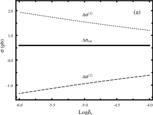
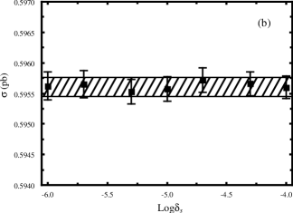
Figure 5: (a) The dependence of the QCD NLO corrections to the $pp\to u\bar{d}\to W_{H}^{+}Z_{H}+X$ process on the cutoffs $\delta_{s}$ and $\delta_{c}$ at the $\sqrt{s}=14~{}{\rm TeV}$ LHC, where we take $f=600~{}{\rm GeV}$, $\kappa=1$, $\delta_{c}=\delta_{s}/100$ and $\mu=\mu_{0}=390.20~{}{\rm GeV}$. (b) The amplified curve for $\Delta\sigma_{tot}$ in Fig.5(a). The shadowing region shows the result by adopting the DPS method with $\pm 1\sigma$ statistic error.

IV..3 Dependence on factorization/renormalization scale

In order to investigate whether the production rates for the $pp\to W_{H}^{+}Z_{H}+X$ and $pp\to W_{H}^{-}Z_{H}+X$ processes at the $\sqrt{s}=14~{}{\rm TeV}$ and the $\sqrt{s}=8~{}{\rm TeV}$ LHC have the stabilization of the dependence on the unphysical renormalization and the factorization scales, we present Figs.6(a) and (b) to describe the cross sections as functions of the renormalization and the factorization scales varied independently and simultaneously. We show the cross section profile both at the LO and at the QCD NLO by adopting the event selection scheme (II) and taking the LHT parameters $f=1~{}{\rm TeV}$ and $\kappa=1$. The curves of the $\sigma_{LO}$ and $\sigma_{NLO}$ for the $pp\to W_{H}^{+}Z_{H}+X$ process are labeled by ”$LO_{+}$” and ”$NLO_{+}$”, while those for the $pp\to W_{H}^{-}Z_{H}+X$ process are labeled by ”$LO_{-}$” and ”$NLO_{-}$”, respectively. The two figures trace the scale dependence following a contour in the $\mu_{R}-\mu_{F}$ plane as shown in each left panel of Figs.6(a) and (b). From these figures we can see that the QCD NLO corrections do not obviously improve the scale uncertainty with individual variation of either $\mu_{R}$ or $\mu_{F}$. Particularly, the LO partonic processes for the $pp\to W_{H}^{\pm}Z_{H}+X$ processes are pure electroweak channels where the $\mu_{R}$ dependence is invisible at the LO, as shown in Figs.6(a)-(3), (a)-(5), (b)-(3) and (b)-(5). Figs.6(a)-(1) and (b)-(1) show that the scale uncertainty is reduced by the NLO corrections with simultaneous variation of $\mu_{R}$ and $\mu_{F}$. It demonstrates that when we set $\mu_{R}=\mu_{F}$ and vary both scales simultaneously, it may lead to artificial cancelations among renormalization and factorization logarithms, and thus hiding the scale dependence. In the following discussions the factorization/renormalization scale is fixed as $\mu_{0}=(m_{W_{H}}+m_{Z_{H}})/2$.

Figure 6: Profile of the renormalization and factorization scale dependence of the LO and NLO corrected cross sections for the processes $pp\to W_{H}^{+}Z_{H}+X$ and $pp\to W_{H}^{-}Z_{H}+X$. The two plots trace the scale dependence following a contour in the $\mu_{R}-\mu_{F}$ plane. There we take the (II) selection scheme and assume $\mu/\mu_{0}=0.2-5$, the LHT parameters $f=1~{}{\rm TeV}$ and $\kappa=1$. (a) at the $\sqrt{s}=14~{}{\rm TeV}$ LHC. (b) at the $\sqrt{s}=8~{}{\rm TeV}$ LHC.

IV..4 Dependence on global symmetry breaking scale $f$

We depict the LO, QCD NLO corrected integrated cross sections and the corresponding $K$-factors for the $pp\to W_{H}^{+}Z_{H}+X$ and $pp\to W_{H}^{-}Z_{H}+X$ processes as functions of the global symmetry breaking scale $f$ at the $\sqrt{s}=14~{}{\rm TeV}$ and the $\sqrt{s}=8~{}{\rm TeV}$ LHC in Figs.7(a), (b), (c) and (d), respectively, with $\kappa=1$. The curves labeled by ”NLO I” and ”NLO II” are for the QCD NLO corrected cross sections using the (I) and (II) selection schemes, respectively. Figs.7(a,b,c,d) demonstrate that the LO and QCD NLO corrected total cross sections for the $pp\to W_{H}^{\pm}Z_{H}+X$ processes decrease sensitively with the increment of $f$ due to the fact that the masses of final $W_{H}$ and $Z_{H}$ become heavier and consequently the phase space becomes smaller as the increment of $f$. The numerical results for the $pp\to W_{H}^{\pm}Z_{H}+X$ processes at the LHC for some typical values of $f$ are presented in Table 2.

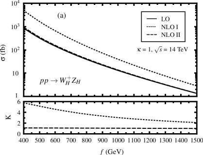
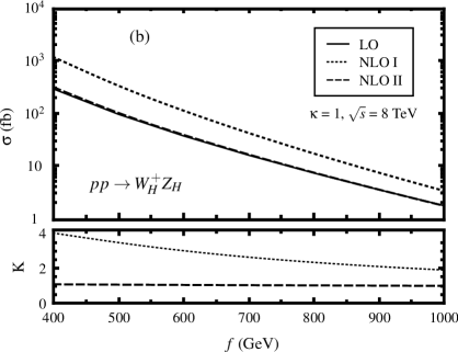
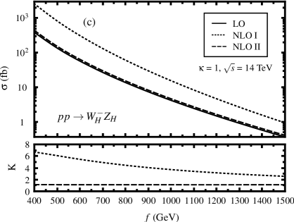
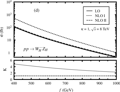
Figure 7: The LO, QCD NLO corrected integrated cross sections and the corresponding $K$-factors as the functions of the global symmetry breaking scale $f$ with $\kappa=1$. (a) for the $pp\to W_{H}^{+}Z_{H}+X$ process at $\sqrt{s}=14~{}{\rm TeV}$ LHC. (b) for the $pp\to W_{H}^{+}Z_{H}+X$ process at $\sqrt{s}=8~{}{\rm TeV}$ LHC. (c) for the $pp\to W_{H}^{-}Z_{H}+X$ process at $\sqrt{s}=14~{}{\rm TeV}$ LHC. (d) for the $pp\to W_{H}^{-}Z_{H}+X$ process at $\sqrt{s}=8~{}{\rm TeV}$ LHC.

$\sqrt{s}$	$f$	$\sigma_{LO}^{(W^{+})}$	$\sigma_{NLO}^{(W^{+})}$	$K^{(W^{+})}$	$\sigma_{LO}^{(W^{-})}$	$\sigma_{NLO}^{(W^{-})}$	$K^{(W^{-})}$
$({\rm TeV})$	$({\rm GeV})$	$({\rm fb})$	$({\rm fb})$		$({\rm fb})$		$({\rm fb})$
	500	321.096(8)	350.8(1)	1.09	136.130(5)	153.12(7)	1.12
	700	72.055(2)	77.26(3)	1.07	26.888(1)	30.03(1)	1.12
14	900	21.9589(5)	23.159(7)	1.05	7.3867(3)	8.216(3)	1.11
	1100	7.8997(2)	8.203(3)	1.04	2.44038(9)	2.709(1)	1.11
	500	94.168(2)	100.01(5)	1.06	32.379(1)	36.10(4)	1.11
8	700	15.7549(4)	16.259(7)	1.03	4.6757(2)	5.192(6)	1.11
	900	3.49785(8)	3.515(1)	1.01	0.93703(3)	1.044(1)	1.11

Table 2: The numerical results of $\sigma_{LO}^{W^{+}}$, $\sigma_{NLO}^{W^{+}}$, $\sigma_{NLO}^{W^{-}}$, $\sigma_{NLO}^{W^{-}}$ for the $pp\to W_{H}^{+}Z_{H}+X$ and $pp\to W_{H}^{-}Z_{H}+X$ processes and their corresponding $K$-factors at the $\sqrt{s}=14~{}{\rm TeV}$ and the $\sqrt{s}=8~{}{\rm TeV}$ LHC by adopting the event selection scheme (II) and taking $\kappa=1$, $\mu=\mu_{0}$ for some typical values of $f$.

IV..5 Differential cross sections

In this subsection we focus on the kinematic distributions of final decay products. The $W_{H}Z_{H}$ associated production at the LHC are followed by the heavy gauge boson decays of $W_{H}^{\mp}\to W^{\mp}A_{H}\to\mu^{\mp}\stackrel{{\scriptstyle(-)}}{{\nu_{\mu}}}A_{H}$ and $Z_{H}\to HA_{H}$. The branching ratios of decays for the $W_{H}$ boson, $Z_{H}$ boson and $W$ boson are taken as $Br(W_{H}\to WA_{H})=100\%$, $Br(Z_{H}\to HA_{H})=100\%$ for $\kappa=1$ and $f=1~{}{\rm TeV}$ [16] and $Br(W^{\mp}\to\mu^{\mp}\stackrel{{\scriptstyle(-)}}{{\nu_{\mu}}})=10.57\%$ [26], respectively. In the following we consider the $W_{H}Z_{H}$ production channel including its subsequential decays as

$$pp\to W_{H}^{\mp}Z_{H}\to W^{\mp}A_{H}HA_{H}\to\mu^{\mp}\stackrel{{\scriptstyle(-)}}{{\nu_{\mu}}}A_{H}HA_{H}.$$ (4.8)

Thus one expects that the $W_{H}Z_{H}$ production at the LHC could be detected via the $\mu^{\mp}H+\not{E}_{T}$ ($\not{E}_{T}$ = transverse energy of $\stackrel{{\scriptstyle(-)}}{{\nu_{\mu}}}+2A_{H}$) channel.

The LO, QCD NLO corrected transverse momentum distributions of $W$ boson and the light neutral Higgs boson $H$ for the $pp\to W_{H}^{+}Z_{H}+X$ and $pp\to W_{H}^{-}Z_{H}+X$ processes, and the corresponding $K$-factors in scheme (II) at the $\sqrt{s}=14~{}{\rm TeV}$ LHC and the $\sqrt{s}=8~{}{\rm TeV}$ LHC are presented in Figs.8(a,b,c,d) and Figs.9(a,b,c,d) separately. There we take $f=1~{}{\rm TeV}$ and $\kappa=1$. From these four figures we find that the QCD NLO corrections enhance the LO transverse momentum distributions in most plotted ranges of $p_{T}$, and the $K$-factors are all less than $1.20$. The maxima of the distributions $\frac{d\sigma_{LO,NLO}}{dp_{T}^{W}}$ and $\frac{d\sigma_{LO,NLO}}{dp_{T}^{H}}$ are all located at about $p_{T}\sim 220~{}{\rm GeV}$.

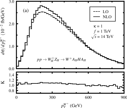
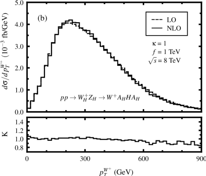
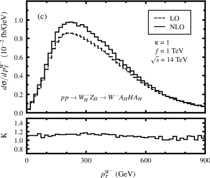
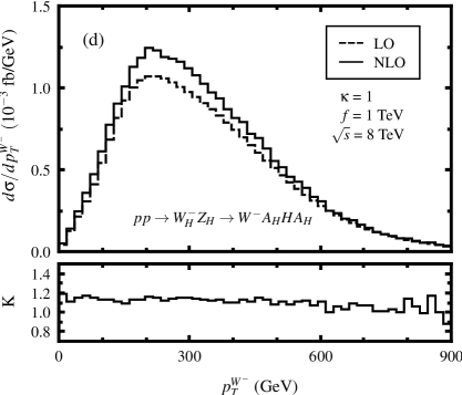
Figure 8: The LO, QCD NLO corrected $p_{T}^{W}$ distributions and the corresponding $K$-factors in scheme (II) for the $pp\to W_{H}^{\pm}Z_{H}\to W^{\pm}A_{H}HA_{H}+X$ processes by taking $f=1~{}{\rm TeV}$ and $\kappa=1$. (a) for the $pp\to W^{+}_{H}Z_{H}\to W^{+}A_{H}HA_{H}+X$ process at the $\sqrt{s}=14~{}{\rm TeV}$ LHC. (b) for the $pp\to W^{+}_{H}Z_{H}\to W^{+}A_{H}HA_{H}+X$ process at the $\sqrt{s}=8~{}{\rm TeV}$ LHC. (c) for the $pp\to W^{-}_{H}Z_{H}\to W^{-}A_{H}HA_{H}+X$ process at the $\sqrt{s}=14~{}{\rm TeV}$ LHC. (d) for the $pp\to W^{-}_{H}Z_{H}\to W^{-}A_{H}HA_{H}+X$ process at the $\sqrt{s}=8~{}{\rm TeV}$ LHC.

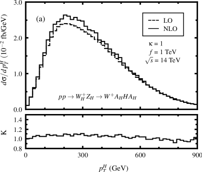
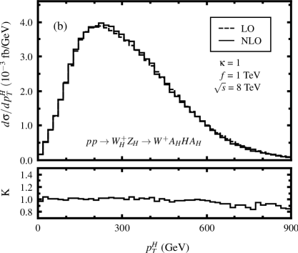
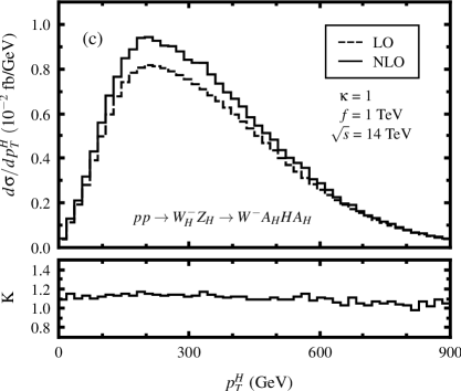
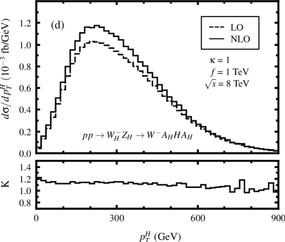
Figure 9: The LO, QCD NLO corrected $p_{T}^{H}$ distributions and the corresponding $K$-factors in scheme (II) for the $pp\to W_{H}^{\pm}Z_{H}\to W^{\pm}A_{H}HA_{H}+X$ processes by taking $f=1~{}{\rm TeV}$ and $\kappa=1$. (a) for the $pp\to W_{H}^{+}Z_{H}\to W^{+}A_{H}HA_{H}+X$  process at $\sqrt{s}=14~{}{\rm TeV}$ LHC. (b) for the $pp\to W_{H}^{+}Z_{H}\to W^{+}A_{H}HA_{H}+X$  process at $\sqrt{s}=8~{}{\rm TeV}$ LHC. (c) for the $pp\to W_{H}^{-}Z_{H}\to W^{-}A_{H}HA_{H}+X$  process at $\sqrt{s}=14~{}{\rm TeV}$ LHC. (d) for the $pp\to W_{H}^{-}Z_{H}\to W^{-}A_{H}HA_{H}+X$  process at $\sqrt{s}=8~{}{\rm TeV}$ LHC.

The LO and QCD NLO corrected transverse momentum distributions of the final $\mu$-lepton and missing energy ($A_{H}A_{H}\stackrel{{\scriptstyle(-)}}{{\nu_{\mu}}}$) for the $pp\to W_{H}^{-}Z_{H}\to\mu^{-}\bar{\nu}A_{H}HA_{H}+X$ and $pp\to W_{H}^{+}Z_{H}\to\mu^{+}\nu_{\mu}A_{H}HA_{H}+X$ processes, and the corresponding $K$-factors in scheme (II) at the early LHC and the future LHC are depicted in Figs.10(a,b,c,d) and Figs.11(a,b,c,d), respectively. There we take $f=1~{}{\rm TeV}$ and $\kappa=1$. Figs.10(a,b) are for the $p_{T}$ distributions of $\mu^{-}$, and Figs.10(c,d) for $\mu^{+}$, respectively. Figs.10 (a), (b), (c) and (d) demonstrate that both the LO and the QCD NLO corrected $p_{T}^{\mu}$ distributions at both the early LHC and the future LHC decrease rapidly with the increment of $p_{T}^{\mu}$. Figs.11(a,b,c,d) show that the LO and NLO missing transverse momentum distributions reach their maxima at $p_{T}^{miss}\sim 290~{}{\rm GeV}$.

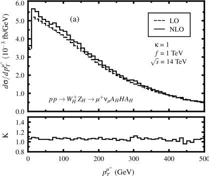
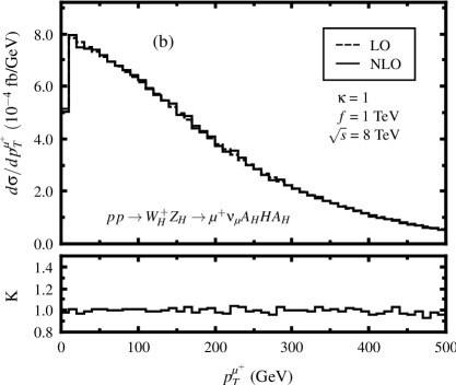
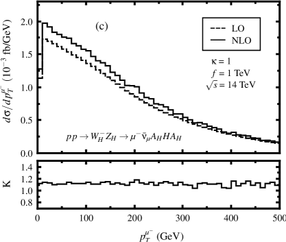
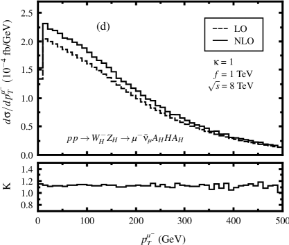
Figure 10: The LO, QCD NLO corrected $p_{T}^{\mu}$ distributions and the corresponding $K$-factors in scheme (II) for the $pp\to W_{H}^{\pm}Z_{H}\to\mu^{\pm}\stackrel{{\scriptstyle(-)}}{{\nu_{\mu}}}A_{H}HA_{H}+X$ processes by taking $f=1~{}{\rm TeV}$ and $\kappa=1$. (a) for the $pp\to W_{H}^{+}Z_{H}\to\mu^{+}{\nu_{\mu}}A_{H}HA_{H}+X$  process at $\sqrt{s}=14~{}{\rm TeV}$ LHC. (b) for the $pp\to W_{H}^{+}Z_{H}\to\mu^{+}{\nu_{\mu}}A_{H}HA_{H}+X$  process at $\sqrt{s}=8~{}{\rm TeV}$ LHC. (c) for the $pp\to W_{H}^{-}Z_{H}\to\mu^{-}\bar{\nu}_{\mu}A_{H}HA_{H}+X$  process at $\sqrt{s}=14~{}{\rm TeV}$ LHC. (d) for the $pp\to W_{H}^{-}Z_{H}\to\mu^{-}\bar{\nu}_{\mu}A_{H}HA_{H}+X$  process at $\sqrt{s}=8~{}{\rm TeV}$ LHC.

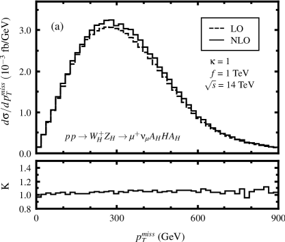
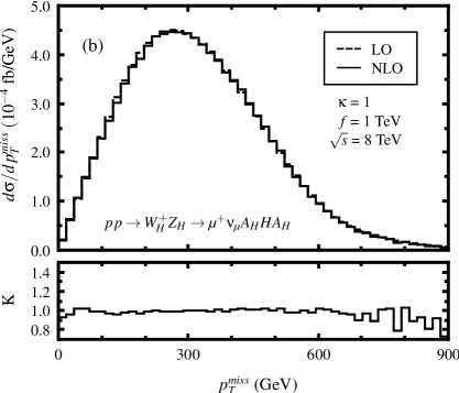
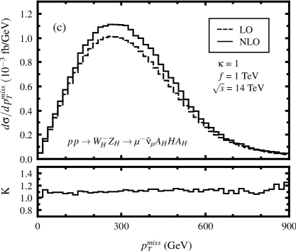
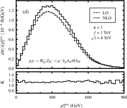
Figure 11: The LO, QCD NLO corrected $p_{T}^{miss}$ distributions and the corresponding $K$-factors in scheme (II) for the $pp\to W_{H}^{\pm}Z_{H}\to\mu^{\pm}\stackrel{{\scriptstyle(-)}}{{\nu_{\mu}}}A_{H}HA_{H}+X$ processes by taking $f=1~{}{\rm TeV}$ and $\kappa=1$. (a) for the $pp\to W_{H}^{+}Z_{H}\to\mu^{+}{\nu_{\mu}}A_{H}HA_{H}+X$  process at the $\sqrt{s}=14~{}{\rm TeV}$ LHC. (b) for the $pp\to W_{H}^{+}Z_{H}\to\mu^{+}{\nu_{\mu}}A_{H}HA_{H}+X$  process at the $\sqrt{s}=8~{}{\rm TeV}$ LHC. (c) for the $pp\to W_{H}^{-}Z_{H}\to\mu^{-}\bar{\nu}_{\mu}A_{H}HA_{H}+X$  process at the $\sqrt{s}=14~{}{\rm TeV}$ LHC. (d) for the $pp\to W_{H}^{-}Z_{H}\to\mu^{-}\bar{\nu}_{\mu}A_{H}HA_{H}+X$  process at the $\sqrt{s}=8~{}{\rm TeV}$ LHC.

To show how the ${\cal O}(\alpha_{s})$ contributions correct the LO differential cross sections at the future and early LHC, we depict the LO, QCD NLO corrected rapidity distributions of final $W$-boson and Higgs boson ($|y_{W}|$ and $|y_{H}|$) for the $W_{H}^{\pm}Z_{H}$ production processes in Figs.12(a,b,c,d) and Figs.13(a,b,c,d), respectively. The $W^{+}$ and Higgs boson rapidity distributions of the $pp\to W_{H}^{+}Z_{H}\to W^{+}A_{H}HA_{H}+X$ process at the future and early LHC are depicted in Figs.12(a,b) and Figs.13(a,b), respectively. Figs.12(c,d) and Figs.13(c,d) provide the $|y_{W^{-}}|$ and $|y_{H}|$ distributions of the $pp\to W_{H}^{-}Z_{H}\to W^{-}A_{H}HA_{H}+X$ process, which offer the comparisons with Figs.12(a,b) and Figs.13(a,b) correspondingly. The rapidity distributions of the final $\mu$-lepton ($|y_{\mu}|$) at the LO and QCD NLO are presented in Figs.14(a,b,c,d). The $y_{\mu^{+}}$ distributions for the $pp\to W_{H}^{+}Z_{H}\to\mu^{+}{\nu_{\mu}}A_{H}HA_{H}+X$  process at the $\sqrt{s}=14~{}{\rm TeV}$ and $\sqrt{s}=8~{}{\rm TeV}$ LHC are plotted in Figs.14(a,b) separately, while the $y_{\mu^{-}}$ distributions for the $pp\to W_{H}^{-}Z_{H}\to\mu^{-}\bar{\nu}_{\mu}A_{H}HA_{H}+X$  process at the $\sqrt{s}=14~{}{\rm TeV}$ and $\sqrt{s}=8~{}{\rm TeV}$ LHC are shown in Figs.14(c,d) respectively. All these figures are obtained by taking the LHT parameters $f=1~{}{\rm TeV}$, $\kappa=1$ and adopting the event selection scheme (II). The corresponding $K$-factors are also plotted in each nether plot of Figs.12, Figs.13 and Figs.14. We can see from all these figures that the QCD NLO corrections do not make shape change in the rapidity distributions.

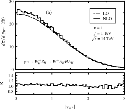
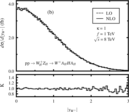
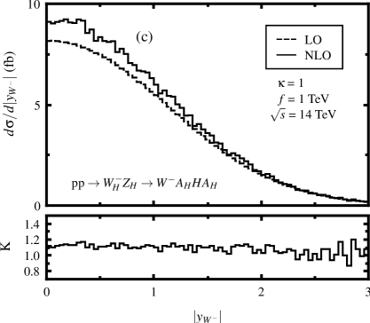
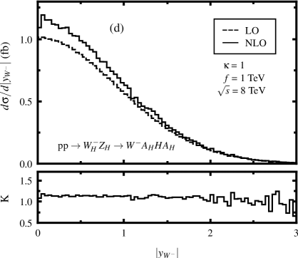
Figure 12: The LO, QCD NLO corrected rapidity distributions of the of final $W$-boson, $|y_{W}|$, and the corresponding $K$-factors in scheme (II) for the $pp\to W^{\pm}_{H}Z_{H}\to W^{\pm}A_{H}HA_{H}+X$ processes by taking $f=1~{}{\rm TeV}$ and $\kappa=1$. (a) for the $pp\to W_{H}^{+}Z_{H}\to W^{+}A_{H}HA_{H}+X$ process at the $\sqrt{s}=14~{}{\rm TeV}$ LHC. (b) for the $pp\to W_{H}^{+}Z_{H}\to W^{+}A_{H}HA_{H}+X$ process at the $\sqrt{s}=8~{}{\rm TeV}$ LHC. (c) for the $pp\to W_{H}^{-}Z_{H}\to W^{-}A_{H}HA_{H}+X$ process at the $\sqrt{s}=14~{}{\rm TeV}$ LHC. (d) for the $pp\to W_{H}^{-}Z_{H}\to W^{-}A_{H}HA_{H}+X$ process at the $\sqrt{s}=8~{}{\rm TeV}$ LHC.

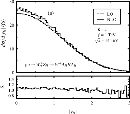
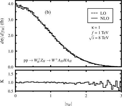
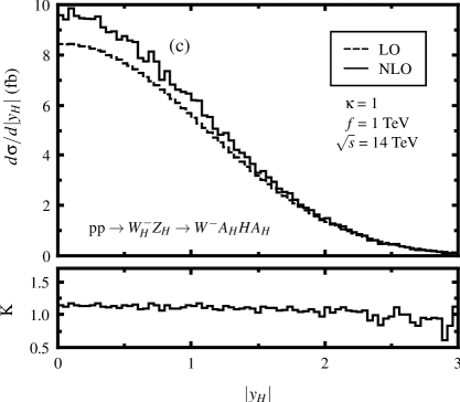
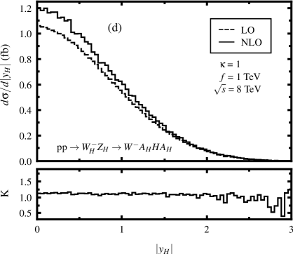
Figure 13: The LO, QCD NLO corrected corrected rapidity distributions of final Higgs boson, $|y_{H}|$, and the corresponding $K$-factors in scheme (II) for the $pp\to W_{H}^{\pm}Z_{H}\to W^{\pm}A_{H}HA_{H}+X$ processes by taking $f=1~{}{\rm TeV}$ and $\kappa=1$. (a) for the $pp\to W_{H}^{+}Z_{H}\to W^{+}A_{H}HA_{H}+X$ process at the $\sqrt{s}=14~{}{\rm TeV}$ LHC. (b) for the $pp\to W_{H}^{+}Z_{H}\to W^{+}A_{H}HA_{H}+X$ process at the $\sqrt{s}=8~{}{\rm TeV}$ LHC. (c) for the $pp\to W_{H}^{-}Z_{H}\to W^{-}A_{H}HA_{H}+X$ process at the $\sqrt{s}=14~{}{\rm TeV}$ LHC. (d) for the $pp\to W_{H}^{-}Z_{H}\to W^{-}A_{H}HA_{H}+X$ process at the $\sqrt{s}=8~{}{\rm TeV}$ LHC.

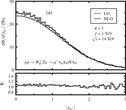
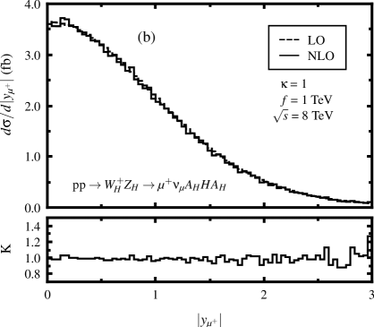
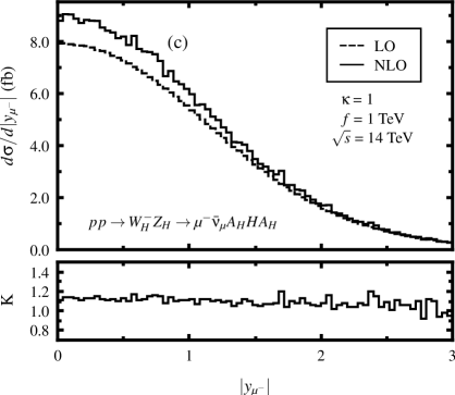
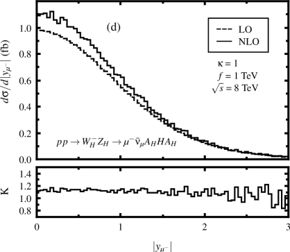
Figure 14: The LO, QCD NLO corrected rapidity distributions of final muon lepton and the corresponding $K$-factors in scheme (II) for the $pp\to W_{H}^{\pm}Z_{H}\to\mu^{\pm}\stackrel{{\scriptstyle(-)}}{{\nu_{\mu}}}A_{H}HA_{H}+X~{}$ processes by taking $f=1~{}{\rm TeV}$ and $\kappa=1$. (a) for the $pp\to W_{H}^{+}Z_{H}\to\mu^{+}{\nu_{\mu}}A_{H}HA_{H}+X$  process at the $\sqrt{s}=14~{}{\rm TeV}$ LHC. (b) for the $pp\to W_{H}^{+}Z_{H}\to\mu^{+}{\nu_{\mu}}A_{H}HA_{H}+X$  process at the $\sqrt{s}=8~{}{\rm TeV}$ LHC. (c) for the $pp\to W_{H}^{-}Z_{H}\to\mu^{-}\bar{\nu}_{\mu}A_{H}HA_{H}+X$  process at the $\sqrt{s}=14~{}{\rm TeV}$ LHC. (d) for the $pp\to W_{H}^{-}Z_{H}\to\mu^{-}\bar{\nu}_{\mu}A_{H}HA_{H}+X$  process at the $\sqrt{s}=8~{}{\rm TeV}$ LHC.

V. Summary

We present the calculations of the $W_{H}Z_{H}$ production at the CERN LHC up to the QCD NLO in the littlest Higgs model with $T$ parity. The dependence of the cross section on the factorization/renormalization scale are investigated theoretically, and the rapidity and transverse momentum distributions of final decay products at both LO and NLO are presented. For the purpose of providing reliable predictions on the $pp\to W_{H}^{\pm}Z_{H}+X~{}$process at the LHC, we adopt two event selection schemes in considering the QCD NLO corrections for comparison. By using the inclusive scheme the perturbative convergence could be destroyed, while we can keep the convergence of the perturbative QCD description and get moderate QCD NLO corrections to the production rate with evidently reduced scale uncertainty by adopting the PROSPINO subtraction scheme and setting $\mu_{F}=\mu_{R}$. With this scheme the QCD NLO correction enhances the LO cross section, and the corresponding $K$-factor for the $W_{H}^{+}Z_{H}$ production process at the future (early) LHC varies in the range of $1.01\sim 1.10$ $(1.00\sim 1.08)$ when $f$ goes from $400~{}{\rm GeV}$ to $1.5~{}{\rm TeV}$ ($1~{}{\rm TeV}$), while the $K$-factor for the $W_{H}^{-}Z_{H}$ production process at the future (early) LHC varies in the range of $1.11\sim 1.13$ ($1.11\sim 1.12$) in the same region of $f$.

Acknowledgments: This work was supported in part by the National Natural Science Foundation of China (Grants No. 11075150, No. 11005101, No. 11275190) and the Fundamental Research Funds for the Central Universities (Grant No. WK2030040024).

VI. Appendix

We list the Feynman rules for the coupling vertices in the LHT related to this work in Table 3 [9, 16, 28, 29], where $P_{L,R}=\frac{1}{2}(1\mp\gamma_{5})$ and $v=v_{SM}$.

Vertex	Feynman rule	Vertex	Feynman rule
$W^{+\mu}(k_{1})W_{H}^{-\nu}(k_{2})Z_{H}^{\rho}(k_{3})$	$i\frac{e}{s_{w}}\left[g^{\mu\nu}(k_{1}-k_{2})^{\rho}+\right.$	$\bar{q}_{-}^{\alpha}q_{-}^{\beta}G_{\mu}^{a}$	$ig_{s}(T^{a})_{\alpha\beta}\gamma_{\mu}$
	$\left.g^{\nu\rho}(k_{2}-k_{3})^{\mu}+g^{\rho\mu}(k_{3}-k_{1})^{\nu}\right]$
$W^{+}_{H\mu}\bar{U}_{i-}D_{j}(i,j=1,2)$	$i\frac{g}{\sqrt{2}}\gamma_{\mu}P_{L}(V_{Hd})_{ij}$	$W^{-}_{H\mu}\bar{D}_{i-}U_{j}(i,j=1,2)$	$i\frac{g}{\sqrt{2}}\gamma_{\mu}P_{L}(V_{Hu})_{ij}$
$Z_{H\mu}\bar{U}_{i-}U_{j}(i,j=1,2)$	$i\left(\frac{gc_{H}}{2}-\frac{g^{\prime}s_{H}}{10}\right)\gamma_{\mu}P_{L}(V_{Hu})_{ij}$	$Z_{H\mu}\bar{D}_{i-}D_{j}(i,j=1,2)$	$i\left(-\frac{gc_{H}}{2}-\frac{g^{\prime}s_{H}}{10}\right)\gamma_{\mu}P_{L}(V_{Hd})_{ij}$

Table 3: The related LHT Feynman rules used in this work, $U_{i}=u,c$, $D_{i}=d,s$, $U_{i-}=u_{-},c_{-}$ and $D_{i-}=d_{-},s_{-}$. $i$ is the generation index.

References

- [1] R. Barbieri and A. Strumia, Phys. Lett. B462, 144 (1999).
- [2] N. Arkani-Hamed, A. G. Cohen and H. Georgi, Phys. Lett. B513, 232 (2001); M. Schmaltz and D. Tucker-Smith, Annu. Rev. Nucl. Part. Sci. 55, 229 (2005); M. Perelstein, Prog. Part. Nucl. Phys. 58, 247 (2007), and references therein.
- [3] S. L. Glashow, Nucl. Phys. 22, 579 (1961); S. Weinberg, Phys. Rev. Lett. 19, 1264 (1967); A. Salam, in Proc. 8th Nobel Symposium Stockholm, 1968, edited by N. Svartholm (Almquist & Wiksells, Stockholm, 1968), p.367; H. D. Politzer, Phys. Rep. 14, 129 (1974).
- [4] P. W. Higgs, Phys. Lett. 12, 132 (1964); Phys. Rev. Lett. 13, 508 (1964); Phys. Rev. 145, 1156 (1966); F. Englert and R. Brout, Phys. Rev. Lett. 13, 321 (1964); G. S. Guralnik, C. R. Hagen and T. W. B. Kibble, Phys. Rev. Lett. 13, 585 (1964); T. W. B. Kibble, Phys. Rev. 155, 1554 (1967).
- [5] C. Csaki, J. Hubisz, G. D. Kribs, P. Meade and J. Terning, Phys. Rev. D67, 115002 (2003).
- [6] ATLAS Collaboration, Phys. Lett. B 705, 28 (2011).
- [7] D. Olivito (ATLAS collaboration), at the Meeting of the Division of Particles and Fields of the American Physical Society (DPF), August 9-13, 2011, Brown University, Providence, Rhode Island (to be published), arXiv:1109.0934.
- [8] I. Low, JHEP 10 (2004) 067.
- [9] J. Hubisz and P. Meade, Phys. Rev. D71, 035016 (2005).
- [10] J. Hubisz, P. Meade, A. Noble and M. Perelstein, JHEP 01 (2006) 135.
- [11] R. Barbieri and A. Strumia, “The ‘LEP paradox’”, arXiv:hep-ph/0007265.
- [12] H. C. Cheng and I. Low, JHEP 09 (2003) 051; 08 (2004) 061.
- [13] A. Birkedal, A. Noble, M. Perelstein and A. Spray, Phys. Rev. D74, 035002 (2006); M. Asano, S. Matsumoto, N. Okada and Y. Okada, Phys. Rev. D75, 063506 (2007).
- [14] R.-Y. Zhang, H. Yan, W.-G. Ma, S.-M. Wang, L. Guo and L. Han, Phys. Rev. D85, 015017 (2012).
- [15] S.-M. Du, L. Guo, W. Liu, W.-G. Ma and R.-Y. Zhang, Phys. Rev. D86, 054027 (2012).
- [16] A. Belyaev, C.-R. Chen, K. Tobe and C.-P. Yuan, Phys. Rev. D74, 115020 (2006).
- [17] Q.-H. Cao and C.-R. Chen, Phys. Rev. D76, 075007 (2007).
- [18] I. Low, W. Skiba and D.Smith, Phys. Rev. D66, 072001 (2002).
- [19] T. Hahn, Comput. Phys. Commun. 140, 418 (2001).
- [20] T. Hahn and M. Perez-Victoria, Comput. Phys. Commun. 118, 153 (1999).
- [21] B. W. Harris and J. F. Owens, Phys. Rev. D65, 094032 (2002).
- [22] T. Kinoshita, J. Math. Phys. (N.Y.) 3, 650 (1962); T. D. Lee and M. Nauenberg, Phys. Rev. 133, B1549 (1964).
- [23] W. Beenakker, R. Höpker, M. Spira and P. M. Zerwas, Nucl. Phys. B492, 51 (1997); W. Beenakker, M. Klasen, M. Krämer, T. Plehn, M. Spira and P. M. Zerwas, Phys. Rev. Lett. 83, 3780 (1999).
- [24] T. Plehn and C. Weydert, Proc. Sci., CHARGED2010 (2010) 026 [arXiv:1012.3761]; T. Binoth, D. Goncalves-Netto, D. Lopez-Val, K. Mawatari, T. Plehn and I. Wigmore, Phys. Rev. D84, 075005 (2011).
- [25] M. Blanke, A. J. Buras, A. Poschenrieder, S. Recksiegel, C. Tarantino, S. Uhlig and A. Weiler, JHEP 01 (2007) 066.
- [26] K. Nakamura et al., J. Phys. G37, 075021 (2010).
- [27] S. Dittmaier, Nucl. Phys. B565, 69 (2000); M. Roth, Ph.D. thesis, ETH Zürich [Institution Report No. 13363, (1999)].
- [28] T. Han, H. E. Logan, B. McElrath and L. T. Wang, Phys. Rev. D67, 095004 (2003).
- [29] K. Pan, R.-Y. Zhang, W.-G. Ma, H. Sun, L. Han and Y. Jiang, Phys. Rev. D76, 015012 (2007).