Variance reduction using antithetic variables for a nonlinear convex stochastic homogenization problem

Abstract

We consider a nonlinear convex stochastic homogenization problem, in a stationary setting. In practice, the deterministic homogenized energy density can only be approximated by a random apparent energy density, obtained by solving the corrector problem on a truncated domain.

We show that the technique of antithetic variables can be used to reduce the variance of the computed quantities, and thereby decrease the computational cost at equal accuracy. This leads to an efficient approach for approximating expectations of the apparent homogenized energy density and of related quantities.

The efficiency of the approach is numerically illustrated on several test cases. Some elements of analysis are also provided.

Keywords: stochastic homogenization, nonlinear problem, variance reduction, antithetic variables.

1 Introduction

In this article, we consider some theoretical and numerical questions related to variance reduction techniques for some nonlinear convex stochastic homogenization problems. In short, we show here that a technique based on antithetic variables can be used in that context, provide some elements of analysis, and demonstrate numerically the efficiency of that approach on several test cases. This work is a follow-up of the articles [5, 6, 10] where the same questions are considered for a linear elliptic equation in divergence form.

The stochastic homogenization problem we consider here writes as follows. Let ${\cal{D}}$ be an open bounded domain of $\mathbb{R}^{d}$ and $2\leq p<\infty$. We consider the highly oscillatory problem

$$\inf\left\{\int_{{\cal{D}}}W\left(\frac{x}{\varepsilon},\omega,\nabla u(x)\right)\,dx-\int_{{\cal{D}}}f(x)u(x)dx,\quad u\in W^{1,p}_{0}({\cal{D}})\right\}$$ (1)

for some $f$ and some random smooth field $W$, which is stationary in a sense made precise below, and satisfies some convexity and growth conditions such that, for any $\varepsilon>0$, problem (1) is well-posed. See Section 1.1 below for a precise description of the mathematical setting, which has been introduced in [11, 12]. A classical example that motivated this framework is when

$$W(y,\omega,\xi)=\frac{1}{p}a\left(y,\omega\right)\left|\xi\right|^{p},$$

where $a$ is stationary (see e.g. [11, page 382]).

In (1), $\varepsilon$ denotes a supposedly small, positive constant that models the smallest possible scale present in the problem. For $\varepsilon$ small, it is extremely expensive, in practice, to directly attack (1) with a numerical discretization. A useful practical approach is to first approximate (1) by its associated homogenized problem, which reads

$$\inf\left\{\int_{{\cal{D}}}W^{\star}\left(\nabla u(x)\right)\,dx-\int_{{\cal{D}}}f(x)u(x)dx,\quad u\in W^{1,p}_{0}({\cal{D}})\right\},$$ (2)

and next numerically solve the latter problem. The two-fold advantage of (2) as compared to (1) is that it is deterministic and it does not involve the small scale $\varepsilon$.

This simplification comes at a price. The homogenized energy density $W^{\star}$ in (2) is given by an integral involving a so-called corrector function, solution to a nonlinear problem (see (7) below for a precise formula). As most often in stochastic homogenization, this corrector problem is set on the entire space $\mathbb{R}^{d}$. In practice, approximations are therefore in order. A standard approach (see e.g. [7] in the linear setting) is to generate realizations of the energy density $W$ over a finite, supposedly large volume at the microscale, that we denote $Q_{N}$, and approach the homogenized energy density by some empirical means using approximate correctors computed on $Q_{N}$. Although the exact homogenized density $W^{\star}$ is deterministic, its practical approximation is random, due to the truncation procedure. It is then natural to generate several realizations. However, efficiently averaging over these realizations require to understand how variance affects the result. This is the purpose of the present article to investigate some questions in this direction, both from the theoretical and numerical standpoints.

Before proceeding and for the sake of consistency, we now present the framework of nonlinear stochastic homogenization we adopt, and situate the questions under consideration in a more general context.

1.1 Homogenization theoretical setting

To begin with, we introduce the basic setting of stochastic homogenization we will employ. We refer to [13] for a general, numerically oriented presentation, and to [4, 9, 17] for classical textbooks. We also refer to [19] and the review article [2] (and the extensive bibliography contained therein) for a presentation of our particular setting. Throughout this article, $(\Omega,{\mathcal{F}},\mathbb{P})$ is a probability space and we denote by $\displaystyle\mathbb{E}(X)=\int_{\Omega}X(\omega)d\mathbb{P}(\omega)$ the expectation value of any random variable $X\in L^{1}(\Omega,d\mathbb{P})$. We next fix $d\in{\mathbb{N}}^{\star}$ (the ambient physical dimension), and assume that the group $(\mathbb{Z}^{d},+)$ acts on $\Omega$. We denote by $(\tau_{k})_{k\in\mathbb{Z}^{d}}$ this action, and assume that it preserves the measure $\mathbb{P}$, that is, for all $\displaystyle k\in\mathbb{Z}^{d}$ and all $A\in{\cal F}$, $\displaystyle\mathbb{P}(\tau_{k}A)=\mathbb{P}(A)$. We assume that the action $\tau$ is ergodic, that is, if $A\in{\mathcal{F}}$ is such that $\tau_{k}A=A$ for any $k\in\mathbb{Z}^{d}$, then $\mathbb{P}(A)=0$ or 1. In addition, we define the following notion of stationarity (see [2, Section 2.2]): a function $F\in L^{1}_{\rm loc}\left(\mathbb{R}^{d},L^{1}(\Omega)\right)$ is said to be stationary if, for all $k\in\mathbb{Z}^{d}$,

$$F(y+k,\omega)=F(y,\tau_{k}\omega)\ \ \text{almost everywhere and almost surely.}$$ (3)

In this setting, the ergodic theorem [18, 22, 24] can be stated as follows: Let $F\in L^{\infty}\left(\mathbb{R}^{d},L^{1}(\Omega)\right)$ be a stationary random variable in the above sense. For $k=(k_{1},k_{2},\dots,k_{d})\in\mathbb{Z}^{d}$, we set $\displaystyle|k|_{\infty}=\sup_{1\leq i\leq d}|k_{i}|$. Then

$$\frac{1}{(2N+1)^{d}}\sum_{|k|_{\infty}\leq N}F(y,\tau_{k}\omega)\mathop{\longrightarrow}_{N\rightarrow\infty}\mathbb{E}\left(F(y,\cdot)\right)\ \ \mbox{in $L^{\infty}(\mathbb{R}^{d})$, almost surely}.$$

This implies that (denoting by $Q$ the unit cube in $\mathbb{R}^{d}$)

$$F\left(\frac{x}{\varepsilon},\omega\right)\mathop{\relbar\joinrel\rightharpoonup}_{\varepsilon\rightarrow 0}^{*}\mathbb{E}\left(\int_{Q}F(y,\cdot)dy\right)\quad\mbox{in $L^{\infty}(\mathbb{R}^{d})$, almost surely}.$$

The purpose of the above setting is simply to formalize that, even though realizations may vary, the function $F$ at point $y\in\mathbb{R}^{d}$ and the function $F$ at point $y+k$, $k\in\mathbb{Z}^{d}$, share the same law. In the homogenization context we now turn to, this means that the local, microscopic environment (encoded in the energy density $W$) is everywhere the same on average. From this, homogenized, macroscopic properties will follow.

We now describe more precisely the multiscale random problem (1). The domain ${\mathcal{D}}$ is a regular (in the sense its boundaries are Lipschitz-continuous) bounded domain of ${\mathbb{R}}^{d}$. The right-hand side function $f$ belongs to $L^{p^{\prime}}({\cal{D}})$, with $1/p+1/p^{\prime}=1$ (hence $f$ is indeed in the dual space of $L^{p}({\cal{D}})$). For any $\xi\in\mathbb{R}^{d}$, the random field $y,\omega\mapsto W(y,\omega,\xi)$ is assumed stationary in the sense (3). We assume that it is continuous (and even $C^{3}$) with respect to the $\xi$ variable, and that it is measurable with respect to the $y$ argument. We also assume that there exists $c_{2}\geq c_{1}>0$ such that

$$\forall y\in\mathbb{R}^{d},\ \ \forall\omega\in\Omega,\ \ \forall\xi\in\mathbb{R}^{d},\quad c_{1}|\xi|^{p}\leq W(y,\omega,\xi)\leq c_{2}(1+|\xi|^{p}).$$ (4)

Furthermore, we assume henceforth that $W$ is strictly convex with respect to the argument $\xi$, in the sense that

$$\forall\eta\in\mathbb{R}^{d},\quad\forall\xi\in\mathbb{R}^{d},\quad\eta^{T}\partial^{2}_{\xi}W(y,\omega,\xi)\eta>0\ \text{ a.e. and a.s.},$$ (5)

where $\partial^{2}_{\xi}W\in\mathbb{R}^{d\times d}$ is the Hessian matrix of $\xi\mapsto W(y,\omega,\xi)$. A more demanding assumption is that $W$ is $\alpha$-convex with respect to the argument $\xi$, in the sense that there exists $\alpha>0$ such that

$$\forall\eta\in\mathbb{R}^{d},\quad\forall\xi\in\mathbb{R}^{d},\quad\eta^{T}\partial^{2}_{\xi}W(y,\omega,\xi)\eta\geq\alpha\,\eta^{T}\eta\ \text{ a.e. and a.s.}$$ (6)

Unless otherwise stated, we only assume (5) in the sequel. When needed, we will explicitly assume (6).

Under (4) and (5), the variational problem (1) is well-posed. In addition, the homogenized limit of (1) has been identified in [11, 12] (see also [14, Theorem 3.1]): the unique solution $u^{\varepsilon}(\cdot,\omega)$ to (1) converges (weakly in $W^{1,p}({\cal{D}})$ and strongly in $L^{p}({\cal{D}})$, almost surely) to some deterministic function $u^{\star}\in W^{1,p}({\cal{D}})$, solution to (2), where the homogenized energy density $W^{\star}$ is given, for any $\xi\in\mathbb{R}^{d}$, by

$$W^{\star}(\xi)=\lim_{N\to\infty}\inf\left\{\frac{1}{|Q_{N}|}\int_{Q_{N}}W\left(y,\omega,\xi+\nabla w(y)\right)\,dy,\quad w\in W^{1,p}_{\#}(Q_{N})\right\}$$ (7)

where $Q_{N}=(-N,N)^{d}$ and where $W^{1,p}_{\#}(Q_{N})$ denotes the set of functions that belong to $W^{1,p}_{\rm loc}(\mathbb{R}^{d})$ and are $Q_{N}$-periodic. The convergence in (7) holds almost surely.

1.2 The questions we consider

In practice, we cannot compute $W^{\star}(\xi)$, and have to restrict ourselves to finite size domains. We therefore introduce

$$W^{\star}_{N}(\omega,\xi):=\inf\left\{\frac{1}{|Q_{N}|}\int_{Q_{N}}W\left(y,\omega,\xi+\nabla w(y)\right)\,dy,\quad w\in W^{1,p}_{\#}(Q_{N})\right\}$$ (8)

and readily see from (7) that

$$W^{\star}(\xi)=\lim_{N\to\infty}W^{\star}_{N}(\omega,\xi)\text{ a.s.}$$

As briefly explained above, although $W^{\star}$ itself is a deterministic object, its practical approximation $W^{\star}_{N}$ is random. It is only in the limit of infinitely large domains $Q_{N}$ that the deterministic value is attained. This is a standard situation in stochastic homogenization.

Many studies have been recently devoted (at least in the linear case) to establishing sharp estimates on the convergence of the random apparent homogenized quantities (computed on $Q_{N}$) to the exact deterministic homogenized quantities. We refer e.g. to [7, 15] and to the comprehensive discussion of [6, Section 1.2]. We take here the problem from a slightly different perspective. We observe that the error

$$W^{\star}(\xi)-W_{N}^{\star}(\omega,\xi)=\Big{(}W^{\star}(\xi)-\mathbb{E}\left[W_{N}^{\star}(\cdot,\xi)\right]\Big{)}+\Big{(}\mathbb{E}\left[W_{N}^{\star}(\cdot,\xi)\right]-W_{N}^{\star}(\omega,\xi)\Big{)}$$

is the sum of a systematic error (the first term in the above right-hand side) and of a statistical error (the second term in the above right-hand side). We focus here on the statistical error, and propose approaches to reduce the confidence interval of empirical means approximating $\mathbb{E}\left[W_{N}^{\star}(\cdot,\xi)\right]$ (or similar quantities), for a given truncated domain $Q_{N}$.

Recall that a standard technique to compute an approximation of $\mathbb{E}\left[W^{\star}_{N}(\cdot,\xi)\right]$ is to consider several independent and identically distributed realizations of the energy density $W$, solve for each of them the corrector problem (8) (thereby obtaining several i.i.d. values $W^{\star,m}_{N}(\omega,\xi)$), and proceed following a Monte Carlo approach:

$$\mathbb{E}\left[W^{\star}_{N}(\cdot,\xi)\right]\approx I_{2M}:=\frac{1}{2M}\sum_{m=1}^{2M}W^{\star,m}_{N}(\omega,\xi).$$

In view of the Central Limit Theorem, we know that our quantity of interest $\mathbb{E}\left[W^{\star}_{N}(\cdot,\xi)\right]$ lies in the confidence interval

$$\left[I_{2M}-1.96\frac{\sqrt{\mathbb{V}{\rm ar}\left[W^{\star}_{N}(\cdot,\xi)\right]}}{\sqrt{2M}},I_{2M}+1.96\frac{\sqrt{\mathbb{V}{\rm ar}\left[W^{\star}_{N}(\cdot,\xi)\right]}}{\sqrt{2M}}\right]$$

with a probability equal to 95 %.

In this article, we show that, using a well known variance reduction technique, the technique of antithetic variables [21, page 27], we can design a practical approach that, for finite $N$ and any vector $\xi$, allows to compute a better approximation of $\mathbb{E}\left[W^{\star}_{N}(\cdot,\xi)\right]$ (and likewise for similar homogenized quantities). Otherwise stated, for an equal computational cost, the approach provides a more accurate (i.e. with a smaller confidence interval) approximation. We thereby extend to this nonlinear convex setting the results of [5, 6, 10] obtained in the linear case.

Our article is articulated as follows. In Section 2.1, we describe the proposed approach, and state our main results. The ingredients to prove these results are collected in Sections 2.2, 2.3 and 2.4. The actual proof of our main results is performed in Section 2.5. We make there several structural assumptions on the form of the energy density $W$ to obtain these variance reduction results. In Section 2.6, we describe a general class of examples for which our assumptions are indeed satisfied. We next turn in Section 3 to some illustrative numerical examples, where we demonstrate the efficiency of the approach, even in cases where the theoretical analysis is incomplete.

2 Description of the proposed approach and main results

2.1 Statement of our main results

This section is devoted to the presentation and the analysis of our approach. We first focus on estimating the expectation $\mathbb{E}\left[W^{\star}_{N}(\cdot,\xi)\right]$ of the apparent homogenized energy density (see Section 2.1.1). Our variance reduction result, Proposition 1, shows that the technique of antithetic variables is indeed efficient. As often the case, it is difficult to quantitatively assess how efficient the approach is, and this will be the purpose of the numerical tests described in Section 3 to address this question.

We then turn to the estimation of the first (and next second) derivatives of $W^{\star}_{N}(\cdot,\xi)$ with respect to $\xi$. These quantities naturally appear when one solves the convex homogenized problem (2) (approximating $W^{*}$ by $W^{\star}_{N}(\omega,\cdot)$), e.g. using a Newton algorithm. For these two quantities, our result is restricted to the one-dimensional setting. See Section 2.1.2 and Proposition 2 for the first derivative, and Section 2.1.3 and Proposition 3 for the second derivative.

Sections 2.2, 2.3, 2.4 and 2.5 are devoted to the proof of the results stated here. In Section 2.6, we discuss an explicit class of energy densities $W$ that falls into our framework.

2.1.1 Variance reduction on the homogenized energy density

In this section, we make the following two structure assumptions on the rapidly oscillating field $W$ of (1). First, we assume that, for any $N$, there exists an integer $n$ (possibly $n=|Q_{N}|$, but not necessarily) and a function ${\cal A}$, defined on $Q_{N}\times\mathbb{R}^{n}\times\mathbb{R}^{d}$, such that the field $W(y,\omega,\xi)$ writes

$$\forall y\in Q_{N},\ \forall\xi\in\mathbb{R}^{d},\quad W(y,\omega,\xi)={\cal A}\left(y,X_{1}(\omega),\ldots,X_{n}(\omega),\xi\right)\quad\text{a.s.},$$ (9)

where $\left\{X_{k}(\omega)\right\}_{1\leq k\leq n}$ are independent scalar random variables, which are all distributed according to the uniform law ${\cal U}[0,1]$. In general, the function ${\cal A}$, as well as the number $n$ of independent, identically distributed variables involved in (9), depend on $N$, the size of $Q_{N}$, although this dependency is not made explicit in (9).

Second, we assume that the function ${\cal A}$ in (9) is such that, for all $y\in Q_{N}$ and all $\xi\in\mathbb{R}^{d}$, the map

$$(x_{1},\ldots,x_{n})\in\mathbb{R}^{n}\mapsto{\cal A}(y,x_{1},\ldots,x_{n},\xi)$$ (10)

is non-decreasing with respect to each of its arguments.

Proposition 1.

We assume (9)–(10). Let $W^{\star}_{N}(\omega,\xi)$ be the approximated homogenized energy density field defined by (8). We define on $Q_{N}$ the field

$$W^{\rm ant}(y,\omega,\xi):={\cal A}(y,1-X_{1}(\omega),\ldots,1-X_{n}(\omega),\xi),$$

antithetic to $W$ defined by (9). We associate to this field the approximate homogenized energy density field $W^{{\rm ant},\star}_{N}(\omega,\xi)$, defined by (8) (replacing $W$ by $W^{\rm ant}$). Set

$$\widetilde{W}^{\star}_{N}(\omega,\xi):=\frac{1}{2}\left(W^{\star}_{N}(\omega,\xi)+W^{{\rm ant},\star}_{N}(\omega,\xi)\right).$$ (11)

Then, for any $\xi\in\mathbb{R}^{d}$,

$$\mathbb{E}\left[\widetilde{W}^{\star}_{N}(\cdot,\xi)\right]=\mathbb{E}\left[W^{\star}_{N}(\cdot,\xi)\right]\ \ \text{and}\ \ \mathbb{V}{\rm ar}\left[\widetilde{W}^{\star}_{N}(\cdot,\xi)\right]\leq\frac{1}{2}\mathbb{V}{\rm ar}\left[W^{\star}_{N}(\cdot,\xi)\right].$$ (12)

Otherwise stated, $\widetilde{W}^{\star}_{N}(\omega,\xi)$ is a random variable which has the same expectation as $W^{\star}_{N}(\omega,\xi)$, and its variance is smaller than half of that of $W^{\star}_{N}(\omega,\xi)$.

As mentioned above, this result generalizes [6, Proposition 2.1] to the nonlinear convex variational setting considered here.

Before proceeding, we briefly explain the usefulness of the above result for variance reduction techniques. Assume we want to compute the expectation of $W^{\star}_{N}(\omega,\xi)$, for some fixed vector $\xi\in\mathbb{R}^{d}$. Following the classical Monte-Carlo method recalled in Section 1.2, we estimate $\mathbb{E}\left[W^{\star}_{N}(\cdot,\xi)\right]$ by its empirical mean. To this end, we consider $2M$ independent, identically distributed copies $\left\{W_{m}(y,\omega,\xi)\right\}_{1\leq m\leq 2M}$ of the random field $W(y,\omega,\xi)$ on $Q_{N}$. To each copy $W_{m}$, we associate an approximate homogenized energy density $W^{\star,m}_{N}(\omega,\xi)$, defined by (8). We next introduce the empirical mean

$$I_{2M}=\frac{1}{2M}\sum_{m=1}^{2M}W^{\star,m}_{N}(\omega,\xi),$$ (13)

and consider that, in practice, the mean $\mathbb{E}\left[W^{\star}_{N}(\cdot,\xi)\right]$ is equal to the estimator $I_{2M}$ within an approximate margin of error $\displaystyle 1.96\frac{\sqrt{\mathbb{V}{\rm ar}\left[W^{\star}_{N}(\cdot,\xi)\right]}}{\sqrt{2M}}$.

Alternate to considering (13), we may consider

$$\widetilde{I}_{2M}=\frac{1}{M}\sum_{m=1}^{M}\widetilde{W}^{\star,m}_{N}(\omega,\xi),$$ (14)

where $\widetilde{W}^{\star,m}_{N}$ is defined by (11). Again, in practice, the mean $\displaystyle\mathbb{E}\left[W^{\star}_{N}(\cdot,\xi)\right]=\mathbb{E}\left[\widetilde{W}^{\star}_{N}(\cdot,\xi)\right]$ is equal to $\widetilde{I}_{2M}$ within an approximate margin of error $\displaystyle 1.96\frac{\sqrt{\mathbb{V}{\rm ar}\left[\widetilde{W}^{\star}_{N}(\cdot,\xi)\right]}}{\sqrt{M}}$. Observe now that both estimators (13) and (14) are of equal cost, since they require the same number $2M$ of corrector problems to be solved. The accuracy of the latter is better if and only if $\displaystyle\mathbb{V}{\rm ar}\left[\widetilde{W}^{\star}_{N}(\cdot,\xi)\right]\leq\frac{1}{2}\mathbb{V}{\rm ar}\left[W^{\star}_{N}(\cdot,\xi)\right]$, which is exactly the bound (12) of Proposition 1.

2.1.2 Variance reduction on the first derivative of the homogenized energy density

Restricting ourselves to the one-dimensional setting, we now state a variance reduction result for the estimation of $\mathbb{E}\left[\xi\partial_{\xi}W^{\star}_{N}(\cdot,\xi)\right]$. Note that, to distinguish derivatives with respect to $y$ from derivatives with respect to $\xi$, we keep the notation $\partial_{\xi}W$, even though we are in the one-dimensional situation.

We again make the structure assumption (9), and observe that it implies that

$$\forall y\in(-N,N),\ \forall\xi\in\mathbb{R},\quad\xi\partial_{\xi}W(y,\omega,\xi)={\cal A}_{1}\left(y,X_{1}(\omega),\ldots,X_{n}(\omega),\xi\right)\quad\text{a.s.},$$

where $\left\{X_{k}(\omega)\right\}_{1\leq k\leq n}$ are scalar i.i.d. random variables, which are all distributed according to the uniform law ${\cal U}[0,1]$, and where the function ${\cal A}_{1}$, defined on $(-N,N)\times\mathbb{R}^{n}\times\mathbb{R}$, is given by

$${\cal A}_{1}(y,x,\xi)=\xi\partial_{\xi}{\cal A}(y,x,\xi).$$ (15)

In addition, we assume that, for all $y\in(-N,N)$ and all $\xi\in\mathbb{R}$, the map

$$(x_{1},\ldots,x_{n})\in\mathbb{R}^{n}\mapsto{\cal A}_{1}(y,x_{1},\ldots,x_{n},\xi)$$ (16)

is non-decreasing with respect to each of its arguments.

We recall that the function $\xi\mapsto W(y,\omega,\xi)$ is strictly convex (see assumption (5)) and satisfies (4). It therefore has a unique minimizer $\xi_{0}(y,\omega)$. In the sequel, we consider energy densities such that this minimizer is independent of $y$ and $\omega$. Without loss of generality, we can assume that $\xi_{0}=0$. We thus consider energy densities $W$ such that

$$\xi\mapsto W(y,\omega,\xi) \xi=0$$ attains its minimum at , a.e. and a.s. (17)

Proposition 2.

Let $d=1$, and assume (9), (15), (16) and (17). We introduce

$$\widetilde{\xi\partial_{\xi}W^{\star}_{N}}(\omega,\xi):=\frac{1}{2}\left(\xi\partial_{\xi}W^{{\rm ant},\star}_{N}\left(\omega,\xi\right)+\xi\partial_{\xi}W^{\star}_{N}\left(\omega,\xi\right)\right),$$ (18)

where $W^{{\rm ant},\star}_{N}\left(\omega,\xi\right)$ and $W^{\star}_{N}\left(\omega,\xi\right)$ are defined as in Proposition 1. Then, for any $\xi\in\mathbb{R}$,

$$\mathbb{E}\left[\widetilde{\xi\partial_{\xi}W^{\star}_{N}}(\cdot,\xi)\right]=\mathbb{E}\left[\xi\partial_{\xi}W^{\star}_{N}(\cdot,\xi)\right]\quad\text{and}\quad\mathbb{V}{\rm ar}\left[\widetilde{\xi\partial_{\xi}W^{\star}_{N}}(\cdot,\xi)\right]\leq\frac{1}{2}\mathbb{V}{\rm ar}\left[\xi\partial_{\xi}W^{\star}_{N}(\cdot,\xi)\right].$$ (19)

2.1.3 Variance reduction on the second derivative of the homogenized energy density

Considering again the one-dimensional setting as in Section 2.1.2, we eventually state a variance reduction result for the estimation of $\mathbb{E}\left[\partial^{2}_{\xi}W^{\star}_{N}(\cdot,\xi)\right]$.

Recall that, for any $y$ and $\omega$, the map $\xi\mapsto\partial_{\xi}W(y,\omega,\xi)$ is increasing. We can therefore introduce its reciprocal function $\zeta\mapsto\psi(y,\omega,\zeta)$, which is also increasing.

We again make the structure assumption (9), and observe that it implies that, for any $y\in(-N,N)$ and any $\zeta\in\mathbb{R}$,

$$\partial^{2}_{\xi}W\left(y,\omega,\psi(y,\omega,\zeta)\right)={\cal A}_{2}(y,X_{1}(\omega),\ldots,X_{n}(\omega),\zeta)\quad\text{a.s.},$$

where $\left\{X_{k}(\omega)\right\}_{1\leq k\leq n}$ are scalar i.i.d. random variables, which are all distributed according to the uniform law ${\cal U}[0,1]$, and where the function ${\cal A}_{2}$, defined on $(-N,N)\times\mathbb{R}^{n}\times\mathbb{R}$, is given by

$${\cal A}_{2}(y,x,\zeta)=\partial^{2}_{\xi}{\cal A}\left(y,x,\left[\partial_{\xi}{\cal A}(y,x,\cdot)\right]^{-1}(\zeta)\right),$$ (20)

where $\zeta\mapsto\left[\partial_{\xi}{\cal A}(y,x,\cdot)\right]^{-1}(\zeta)$ is the reciprocal function of $\xi\mapsto\partial_{\xi}{\cal A}(y,x,\xi)$.

In addition, we assume that, for all $y\in(-N,N)$ and all $\zeta\in\mathbb{R}$, the map

$$(x_{1},\ldots,x_{n})\in\mathbb{R}^{n}\mapsto{\cal A}_{2}(y,x_{1},\ldots,x_{n},\zeta)$$ (21)

is non-decreasing with respect to each of its arguments.

Proposition 3.

Let $d=1$, and assume (9), (15), (16), (20) and (21). We also assume that (17) holds, and that

$$\begin{array}[]{c}\xi\mapsto\partial^{2}_{\xi}W\left(y,\omega,\xi\right)\text{is non decreasing for $\xi\geq 0$}\\ \text{and non increasing for $\xi\leq 0$, a.e. and a.s.}\end{array}$$ (22)

We introduce

$$\widetilde{\partial^{2}_{\xi}W^{\star}_{N}}(\omega,\xi):=\frac{1}{2}\left(\partial^{2}_{\xi}W^{{\rm ant},\star}_{N}\left(\omega,\xi\right)+\partial^{2}_{\xi}W^{\star}_{N}\left(\omega,\xi\right)\right),$$

where $W^{{\rm ant},\star}_{N}\left(\omega,\xi\right)$ and $W^{\star}_{N}\left(\omega,\xi\right)$ are defined as in Proposition 1. Then, for any $\xi\in\mathbb{R}$,

$$\mathbb{E}\left[\widetilde{\partial^{2}_{\xi}W^{\star}_{N}}(\cdot,\xi)\right]=\mathbb{E}\left[\partial^{2}_{\xi}W^{\star}_{N}(\cdot,\xi)\right]\quad\text{and}\quad\mathbb{V}{\rm ar}\left[\widetilde{\partial^{2}_{\xi}W^{\star}_{N}}(\cdot,\xi)\right]\leq\frac{1}{2}\mathbb{V}{\rm ar}\left[\partial^{2}_{\xi}W^{\star}_{N}(\cdot,\xi)\right].$$ (23)

The density $W(y,\omega,\xi)=a(y,\omega)|\xi|^{p}$, where $a$ is positive and bounded away from zero and $p\geq 2$, typically satisfies the assumption (22).

2.2 Classical results on antithetic variables

We first recall the following lemma, and provide its proof for consistency. This result is crucial for our proof of variance reduction using the technique of antithetic variables, performed in Section 2.5.

Lemma 4 ([21], page 27).

Let $f$ and $g$ be two real-valued functions defined on $\mathbb{R}^{n}$, which are non-decreasing with respect to each of their arguments. Consider $X=(X_{1},\ldots,X_{n})$ a vector of random variables, which are all independent from one another. Then

$$\mathbb{C}{\rm ov}(f(X),g(X))\geq 0.$$ (24)

Proof.

This lemma is proved by induction. We treat the one-dimensional case ($n=1$) below, and we refer to [6, Proof of Lemma 2.1] for the induction. Consider $X$ and $Y$ two independent scalar random variables, identically distributed. Both functions $f$ and $g$ are non-decreasing, so

$$(f(X)-f(Y))\ (g(X)-g(Y))\geq 0.$$

We now take the expectation of the above inequality:

$$\mathbb{E}(f(X)\ g(X))+\mathbb{E}(f(Y)\ g(Y))\geq\mathbb{E}(f(Y)\ g(X))+\mathbb{E}(f(X)\ g(Y)).$$

As $X$ and $Y$ share the same law, and are independent, this yields

$$\mathbb{E}(f(X)\ g(X))\geq\mathbb{E}(f(X))\ \mathbb{E}(g(X)),$$

and (24) follows for $n=1$. ∎

The following result is a simple consequence of the above lemma (see e.g. [6] for a proof).

Corollary 5 ([21]).

Let $f$ be a function defined on $\mathbb{R}^{n}$, which is non-decreasing with respect to each of its arguments. Consider $X=(X_{1},\ldots,X_{n})$ a vector of random variables, which are all independent from one another, and distributed according to the uniform law  ${\cal U}[0,1]$. Then

$$\mathbb{V}{\rm ar}\left(\frac{1}{2}\left(f(X)+f(1-X)\right)\right)\leq\frac{1}{2}\mathbb{V}{\rm ar}\left(f(X)\right),$$

where we denote $1-X=(1-X_{1},\ldots,1-X_{n})\in\mathbb{R}^{n}$.

Proof.

Choosing $g(x_{1},\ldots,x_{n})=-f(1-x_{1},\ldots,1-x_{n})$ in Lemma 4, we obtain that

$$\mathbb{C}{\rm ov}(f(X),f(1-X))=\mathbb{C}{\rm ov}(f(X_{1},\ldots,X_{n}),f(1-X_{1},\ldots,1-X_{n}))\leq 0.$$

We next observe that

$$\mathbb{V}{\rm ar}\left(\frac{1}{2}\left(f(X)+f(1-X)\right)\right) = \frac{1}{2}\mathbb{V}{\rm ar}(f(X))+\frac{1}{2}\mathbb{C}{\rm ov}\left(f(X),f(1-X)\right)$$

$$\leq \frac{1}{2}\mathbb{V}{\rm ar}(f(X)),$$

where we have used that $\mathbb{V}{\rm ar}(f(X))=\mathbb{V}{\rm ar}(f(1-X))$. ∎

2.3 Derivatives of the corrector and of the homogenized energy density

We now introduce the correctors as the solutions to (8):

$$w^{N}(\cdot,\omega,\xi):=\text{arginf}\left\{\int_{Q_{N}}W(\cdot,\omega,\xi+\nabla v),\quad v\in W^{1,p}_{\#}(Q_{N}),\quad\int_{Q_{N}}v=0\right\}.$$

In this section, we derive some useful expressions for the derivatives with respect to $\xi$ of $w^{N}$ and of $W^{\star}_{N}$.

The first order optimality condition in (8) reads

$$\forall h\in W^{1,p}_{\#}(Q_{N}),\quad\int_{Q_{N}}\left(\nabla h\right)^{T}\partial_{\xi}W\left(\cdot,\omega,\xi+\nabla w^{N}\right)=0.$$ (25)

We deduce from that condition that

$$\partial_{\xi}W^{\star}_{N}(\omega,\xi)=\frac{1}{|Q_{N}|}\int_{Q_{N}}\partial_{\xi}W\left(\cdot,\omega,\xi+\nabla w^{N}\right),$$ (26)

and we note that we do not need to know $\partial_{\xi}w^{N}$ to compute $\partial_{\xi}W^{\star}_{N}$. Computing the derivative of this equality with respect to $\xi$, we obtain that

$$\partial^{2}_{\xi}W^{\star}_{N}(\omega,\xi)=\frac{1}{|Q_{N}|}\int_{Q_{N}}\left(\text{Id}+\partial_{\xi}\nabla w^{N}\right)\partial^{2}_{\xi}W\left(\cdot,\omega,\xi+\nabla w^{N}\right)$$ (27)

with the convention that $\displaystyle\left[\partial_{\xi}\nabla w^{N}\right]_{jk}=\frac{\partial^{2}w^{N}}{\partial\xi_{j}\partial y_{k}}$ for $1\leq j,k\leq d$. We can actually obtain a somewhat more symmetric expression. Computing the derivative of (25) with respect to $\xi$, we indeed see that

$$\forall h\in W^{1,p}_{\#}(Q_{N}),\quad\int_{Q_{N}}\left(\text{Id}+\partial_{\xi}\nabla w^{N}\right)\partial^{2}_{\xi}W\left(\cdot,\omega,\xi+\nabla w^{N}\right)\nabla h=0.$$ (28)

We then infer from (27) and (28) that

$$\partial_{\xi}^{2}W^{\star}_{N}(\omega,\xi)=\frac{1}{|Q_{N}|}\int_{Q_{N}}\left(\text{Id}+\partial_{\xi}\nabla w^{N}\right)\partial_{\xi}^{2}W\left(\cdot,\omega,\xi+\nabla w^{N}\right)\left(\text{Id}+\partial_{\xi}\nabla w^{N}\right)^{T}.$$ (29)

Remark 6.

Using the same kind of arguments, we see that the function $\displaystyle g_{j}=\frac{\partial w^{N}}{\partial\xi_{j}}\in W^{1,p}_{\#}(Q_{N})$ is solution to the variational formulation

$$\forall h\in W^{1,p}_{\#}(Q_{N}),\quad\int_{Q_{N}}\left(\nabla h\right)^{T}\partial^{2}_{\xi}W\left(\cdot,\omega,\xi+\nabla w^{N}\right)\nabla g_{j}\\ =-\sum_{i=1}^{d}\int_{Q_{N}}\frac{\partial h}{\partial y_{i}}\frac{\partial^{2}W}{\partial\xi_{j}\partial\xi_{i}}\left(\cdot,\omega,\xi+\nabla w^{N}\right).$$ (30)

Suppose that $W$ is $\alpha$-convex (i.e. satisfies (6)). Then problem (30) is well-posed and allows to uniquely determine (up to an additive constant) $g_{j}$, by solving a linear elliptic partial differential equation.

Combined with (29), this remark provides a practical way to compute $\partial_{\xi}^{2}W^{\star}_{N}(\omega,\xi)$ without using any finite difference approximation in $\xi$.

We finally note that, in view of (26), we have

$$\xi\cdot\partial_{\xi}W^{\star}_{N}(\omega,\xi)=\frac{1}{|Q_{N}|}\int_{Q_{N}}\xi\cdot\partial_{\xi}W\left(\cdot,\omega,\xi+\nabla w^{N}\right).$$ (31)

Likewise, in view of (29), we see that

$$\xi^{T}\partial_{\xi}^{2}W^{\star}_{N}(\omega,\xi)\xi=\\ \frac{1}{|Q_{N}|}\int_{Q_{N}}\left[\xi+\nabla\left(\xi\cdot\partial_{\xi}w^{N}\right)\right]^{T}\partial_{\xi}^{2}W\left(\cdot,\omega,\xi+\nabla w^{N}\right)\left[\xi+\nabla\left(\xi\cdot\partial_{\xi}w^{N}\right)\right].$$ (32)

2.4 Monotonicity properties

Our goal in this section is to establish monotonicity properties for the homogenization process. Such properties are indeed useful to apply Corollary 5 and therefore prove variance reduction.

To simplify the notation, we assume in this section that we are in a periodic setting. For any $\xi\in\mathbb{R}^{d}$, the function $y\mapsto W(y,\xi)$ is supposed to be $Q$-periodic (with $Q=(0,1)^{d}$), to satisfy the growth condition (4) and to be strictly convex with respect to $\xi$. The associated homogenized energy density is then given by

$$W^{\star}(\xi)=\inf\left\{\int_{Q}W\left(y,\xi+\nabla w(y)\right)\,dy,\quad w\in W^{1,p}_{\#}(Q),\quad\int_{Q}w=0\right\}.$$ (33)

We first show a monotonicity property on the homogenized energy density in Section 2.4.1. Next, restricting ourselves to the one-dimensional setting, we show monotonicity properties for the first and the second derivative of the homogenized energy density (see respectively Sections 2.4.2 and 2.4.3).

2.4.1 On the homogenized energy density

The following result is an extension to the nonlinear setting of a well-known result in the linear setting (see [23, page 12]).

Lemma 7.

Suppose that the fields $W_{1}$ and $W_{2}$ satisfy

$$\forall\xi\in\mathbb{R}^{d},\quad W_{2}(y,\xi)\geq W_{1}(y,\xi)\text{ a.e. on $Q$}.$$ (34)

We denote $W_{1}^{\star}$ and $W_{2}^{\star}$ the corresponding homogenized energy densities, defined by (33). We then have

$$\forall\xi\in\mathbb{R}^{d},\quad W^{\star}_{2}(\xi)\geq W^{\star}_{1}(\xi).$$ (35)

Proof.

Fix $\xi\in\mathbb{R}^{d}$. For any $v\in W^{1,p}_{\#}(Q)$ with $\displaystyle\int_{Q}v=0$, we have that

$$W^{\star}_{1}(\xi)\leq\int_{Q}W_{1}\left(y,\xi+\nabla v(y)\right)\,dy\leq\int_{Q}W_{2}\left(y,\xi+\nabla v(y)\right)\,dy.$$

Taking the infimum over $v$, we obtain the claimed result. ∎

Remark 8.

Consider the case of an energy density that is positively homogeneous of degree $p$ with respect to its variable $\xi$, that is such that $W(y,\lambda\xi)=|\lambda|^{p}\,W(y,\xi)$ for any $y\in\mathbb{R}^{d}$, $\xi\in\mathbb{R}^{d}$ and $\lambda\in\mathbb{R}$. A typical example is $\displaystyle W(y,\xi)=\frac{1}{p}a(y)|\xi|^{p}$. We then have, for any $y$ and $\xi$, that

$$\xi\cdot\partial_{\xi}W(y,\xi)=pW(y,\xi)\quad\text{and}\quad\xi^{T}\partial^{2}_{\xi}W(y,\xi)\xi=p(p-1)W(y,\xi).$$ (36)

Using successively (31), (25) and (36), we obtain that

$$\xi\cdot\partial_{\xi}W^{\star}(\xi) = \int_{Q}\xi\cdot\partial_{\xi}W\left(\cdot,\xi+\nabla w\right)$$ (37)

$$= \int_{Q}(\xi+\nabla w)\cdot\partial_{\xi}W\left(\cdot,\xi+\nabla w\right)$$

$$= p\int_{Q}W\left(\cdot,\xi+\nabla w\right)$$

$$= pW^{\star}(\xi),$$

where $w$ is the corrector, solution to (33).

We next observe that, for any $\lambda\in\mathbb{R}$, we have $w(\cdot,\lambda\xi)=\lambda w(\cdot,\xi)$. Thus, for any $y$, the map $\xi\mapsto w(y,\xi)$ is homogeneous of degree one, and therefore $\xi\cdot\partial_{\xi}w=w$. We thus infer from (32), using (36), that

$$\xi^{T}\partial_{\xi}^{2}W^{\star}(\xi)\xi = \int_{Q}[\xi+\nabla w]^{T}\partial_{\xi}^{2}W(\cdot,\xi+\nabla w)[\xi+\nabla w]$$ (38)

$$= p(p-1)\int_{Q}W(\cdot,\xi+\nabla w)$$

$$= p(p-1)W^{\star}(\xi).$$

Consider now two fields $W_{1}$ and $W_{2}$ that are positively homogeneous of degree $p$ with respect to the variable $\xi$ and satisfy (34). Then we deduce from (35), (37) and (38) that, for all $\xi\in\mathbb{R}^{d}$,

$$\xi\cdot\partial_{\xi}W_{2}^{\star}(\xi)\geq\xi\cdot\partial_{\xi}W_{1}^{\star}(\xi)\quad\text{and}\quad\xi^{T}\partial_{\xi}^{2}W_{2}^{\star}(\xi)\xi\geq\xi^{T}\partial_{\xi}^{2}W_{1}^{\star}(\xi)\xi.$$

2.4.2 On the first derivative of the homogenized energy density

We now establish a monotonicity result on the derivative of $W^{\star}(\xi)$, in the one-dimensional setting.

As in Section 2.1.2 (see (17)), we consider energy densities $W$ such that

$$\xi\mapsto W(y,\xi) \xi=0 y\in Q$$ attains its minimum at for almost all . (39)

Lemma 9.

Let $d=1$, and consider two energy densities $W_{1}$ and $W_{2}$ satisfying (39), and such that

$$\forall\xi\in\mathbb{R},\quad\xi\partial_{\xi}W_{2}(y,\xi)\geq\xi\partial_{\xi}W_{1}(y,\xi)\text{ a.e. on $(0,1)$}.$$ (40)

We denote $W_{1}^{\star}$ and $W_{2}^{\star}$ the corresponding homogenized energy densities, defined by (33). We then have

$$\forall\xi\in\mathbb{R},\quad\xi\partial_{\xi}W_{2}^{\star}(\xi)\geq\xi\partial_{\xi}W_{1}^{\star}(\xi).$$ (41)

Proof.

We first claim that

$$\partial_{\xi}W^{\star}(\xi) \xi$$ has the same sign as . (42)

To prove this, we note that the corrector equation reads (see (25))

$$\frac{d}{dy}\left[\partial_{\xi}W\left(y,\xi+\frac{dw}{dy}(y,\xi)\right)\right]=0\quad\text{on $(0,1)$},\quad w(\cdot,\xi)\text{ is 1-periodic}.$$

We therefore see that $\displaystyle\partial_{\xi}W\left(y,\xi+\frac{dw}{dy}(y,\xi)\right)$ is independent of $y$, and using (26), we obtain that

$$\partial_{\xi}W\left(y,\xi+\frac{dw}{dy}(y,\xi)\right)=\partial_{\xi}W^{\star}(\xi)\quad\text{on $(0,1)$}.$$

Let $\xi\mapsto\psi(y,\xi)$ be the reciprocal function of $\xi\mapsto\partial_{\xi}W(y,\xi)$, which exists and is increasing thanks to the strict convexity of $\xi\mapsto W(y,\xi)$. We deduce from the above equation, after integration over $(0,1)$, that

$$\xi=\int_{0}^{1}\psi\left(y,\partial_{\xi}W^{\star}(\xi)\right)dy.$$ (43)

We are now in position to prove (42). Indeed, we first note that (39), that reads $\partial_{\xi}W(y,\xi=0)=0$, implies that $\psi(y,0)=0$. If $\partial_{\xi}W^{\star}(\xi)\geq 0$, then $\psi(y,\partial_{\xi}W^{\star}(\xi)\geq\psi(y,0)=0$, hence, integrating over $(0,1)$ and using (43), we obtain $\xi\geq 0$. Likewise, $\partial_{\xi}W^{\star}(\xi)\leq 0$ implies that $\xi\leq 0$. The claim (42) is proved.

To proceed, we see that the assumption (40) equivalently reads, using the reciprocal functions,

$$\forall\zeta\in\mathbb{R},\quad\zeta\psi_{2}(y,\zeta)\leq\zeta\psi_{1}(y,\zeta)\quad\text{a.e. on $(0,1)$}.$$ (44)

We now prove (41) by contradiction. Assume that $\xi\partial_{\xi}W_{2}^{\star}(\xi)<\xi\partial_{\xi}W_{1}^{\star}(\xi)$ for some $\xi\in\mathbb{R}$. Without loss of generality, we can assume that $\xi>0$, and therefore $\partial_{\xi}W_{2}^{\star}(\xi)<\partial_{\xi}W_{1}^{\star}(\xi)$. Using (42), we additionally have $0<\partial_{\xi}W_{2}^{\star}(\xi)$. Using that $\zeta\mapsto\psi_{2}(y,\zeta)$ is increasing and (44) with $\zeta=\partial_{\xi}W_{1}^{\star}(\xi)>0$, we have

$$\psi_{2}\left(y,\partial_{\xi}W_{2}^{\star}(\xi)\right)<\psi_{2}\left(y,\partial_{\xi}W_{1}^{\star}(\xi)\right)\leq\psi_{1}\left(y,\partial_{\xi}W_{1}^{\star}(\xi)\right).$$

Integrating over $(0,1)$ and using (43) yields

$$\xi=\int_{0}^{1}\psi_{2}\left(y,\partial_{\xi}W_{2}^{\star}(\xi)\right)dy<\int_{0}^{1}\psi_{1}\left(y,\partial_{\xi}W_{1}^{\star}(\xi)\right)dy=\xi,$$

and we reach a contradiction. This concludes the proof. ∎

2.4.3 On the second derivative of the homogenized energy density

We next turn to monotonicity properties of the second derivative of the homogenized energy density. As in Section 2.4.2, we consider energy densities satisfying (39). We additionally request that, almost everywhere in $(0,1)$,

$$\begin{array}[]{c}\xi\mapsto\partial^{2}_{\xi}W\left(y,\xi\right)\text{is non decreasing for $\xi\geq 0$}\\ \text{and non increasing for $\xi\leq 0$.}\end{array}$$ (45)

Lemma 10.

Let $d=1$, and consider two energy densities $W_{1}$ and $W_{2}$ satisfying (39), (40), (45) and such that

$$\forall\zeta\in\mathbb{R},\quad\partial^{2}_{\xi}W_{2}\left(y,\psi_{2}(y,\zeta)\right)\geq\partial^{2}_{\xi}W_{1}\left(y,\psi_{1}(y,\zeta)\right)\text{ a.e. on $(0,1)$}.$$ (46)

We denote $W_{1}^{\star}$ and $W_{2}^{\star}$ the corresponding homogenized energy densities, defined by (33). We then have

$$\forall\xi\in\mathbb{R},\quad\partial^{2}_{\xi}W_{2}^{\star}(\xi)\geq\partial^{2}_{\xi}W_{1}^{\star}(\xi).$$ (47)

We recall that $\zeta\mapsto\psi(y,\zeta)$ is the reciprocal function of $\xi\mapsto\partial_{\xi}W(y,\xi)$.

Proof.

We first compute the derivative of (43) and obtain

$$\frac{1}{\partial^{2}_{\xi}W^{\star}(\xi)}=\int_{0}^{1}\frac{dy}{\partial^{2}_{\xi}W\left[y,\psi\left(y,\partial_{\xi}W^{\star}(\xi)\right)\right]}.$$ (48)

It is sufficient to prove (47) for $\xi>0$. Using (41) and the fact that $\psi_{1}$ and $\partial^{2}_{\xi}W_{1}$ are non-decreasing with respect to their second argument, we have

$$\partial^{2}_{\xi}W_{1}\left(y,\psi_{1}\left(y,\partial_{\xi}W_{1}^{\star}(\xi)\right)\right)\leq\partial^{2}_{\xi}W_{1}\left(y,\psi_{1}\left(y,\partial_{\xi}W_{2}^{\star}(\xi)\right)\right).$$

Using (46) for $\zeta=\partial_{\xi}W_{2}^{\star}(\xi)$, we deduce that

$$\partial^{2}_{\xi}W_{1}\left(y,\psi_{1}\left(y,\partial_{\xi}W_{1}^{\star}(\xi)\right)\right)\leq\partial^{2}_{\xi}W_{2}\left(y,\psi_{2}\left(y,\partial_{\xi}W_{2}^{\star}(\xi)\right)\right).$$

In view of (48), this inequality readily implies (47) for $\xi>0$. This concludes the proof. ∎

2.5 Proof of Propositions 1, 2 and 3

Now that we have collected all the necessary ingredients, we are in position to prove our main results.

2.5.1 Variance reduction on the homogenized energy density

Proof of Proposition 1.

As $1-X_{k}(\omega)$ and $X_{k}(\omega)$ share the same law, so do the fields $W$ and $W^{\text{ant}}$ on $Q_{N}$. Hence, the homogenized fields $W^{\star}_{N}(\omega,\xi)$ and $W^{{\rm ant},\star}_{N}(\omega,\xi)$ share the same law, and we obtain the first assertion of (12).

We now choose a vector $\xi\in\mathbb{R}^{d}$, and denote by $\mathcal{P}^{\xi}_{N}$ the operator that associates to a given $Q_{N}$-periodic energy density the homogenized energy density evaluted at $\xi$. We see from (8) that $W^{\star}_{N}(\omega,\xi)$ is the effective energy density (evaluated at $\xi$) obtained by periodic homogenization of $W_{|y\in Q_{N}}$:

$$W^{\star}_{N}(\omega,\xi)=\mathcal{P}^{\xi}_{N}\left[W(\cdot,\omega,\cdot)_{|y\in Q_{N}}\right]\quad\text{a.s.}$$ (49)

Using the function ${\cal A}$ of (9), we introduce the map

$$f:\mathbb{R}^{n} \to \mathbb{R}$$

$$x \mapsto \mathcal{P}^{\xi}_{N}\left[{\cal A}(\cdot,x,\cdot)\right],$$

see that $f(X(\omega))=W^{\star}_{N}(\omega,\xi)$ and that, using the definition (11) of $\widetilde{W}^{\star}_{N}(\omega,\xi)$, we have

$$\frac{1}{2}\left(f(X(\omega))+f(1-X(\omega))\right)=\frac{1}{2}\left(W^{\star}_{N}(\omega,\xi)+W^{{\rm ant},\star}_{N}(\omega,\xi)\right)=\widetilde{W}^{\star}_{N}(\omega,\xi).$$ (50)

We now infer from Assumption (10) that, for any $y\in Q_{N}$ and any $\zeta\in\mathbb{R}^{d}$, the function ${\cal A}(y,\cdot,\zeta)$ is non-decreasing with respect to each of its arguments. In view of Lemma 7, we obtain that $f$ is non-decreasing.

We are thus in position to use Corollary 5, which yields

$$\mathbb{V}{\rm ar}\left(\frac{1}{2}\left(f(X)+f(1-X)\right)\right)\leq\frac{1}{2}\mathbb{V}{\rm ar}\left(f(X)\right).$$

Using (50), we obtain

$$\mathbb{V}{\rm ar}\left(\widetilde{W}^{\star}_{N}(\cdot,\xi)\right)\!=\!\mathbb{V}{\rm ar}\left[\frac{1}{2}\left(f(X)+f(1-X)\right)\right]\!\leq\!\frac{1}{2}\mathbb{V}{\rm ar}\left(f(X)\right)\!=\!\frac{1}{2}\mathbb{V}{\rm ar}\left(W^{\star}_{N}(\cdot,\xi)\right),$$

which concludes the proof of the second assertion of (12) and of the Proposition 1. ∎

Remark 11.

Following Remark 8, consider a positively homogeneous energy density $W$. We have shown there that $\xi\cdot\partial_{\xi}W_{N}^{\star}(\omega,\xi)$ and $\xi^{T}\partial^{2}_{\xi}W_{N}^{\star}(\omega,\xi)\xi$ are equal (up to a multiplicative constant) to $W_{N}^{\star}(\omega,\xi)$. Thus, under Assumptions (9)–(10), variance reduction holds for these two outputs as well.

2.5.2 Variance reduction on the first derivative of the homogenized energy density

Proof of Proposition 2.

The proof follows the same lines as that of Proposition 1.

As $1-X_{k}(\omega)$ and $X_{k}(\omega)$ share the same law, so do the fields $W$ and $W^{\rm ant}$ on $Q_{N}$. Hence, the quantities $\xi\partial_{\xi}W^{\star}_{N}(\omega,\xi)$ and $\xi\partial_{\xi}W^{{\rm ant},\star}_{N}(\omega,\xi)$ share the same law, which implies the first assertion of (19).

To prove the second assertion, we again make use, as in the proof of Proposition 1, of the operator ${\mathcal{P}}^{\xi}_{N}$ that associates to a given $Q_{N}$-periodic energy density the homogenized energy density evaluted at $\xi$ (here, $Q_{N}=(-N,N)$). Expression (49) holds. Choosing a vector $\xi\in\mathbb{R}$, we introduce the function

$$f:\mathbb{R}^{n} \to \mathbb{R}$$

$$x \mapsto \xi\partial_{\xi}\left[{\mathcal{P}}^{\xi}_{N}\left({\cal A}(\cdot,x,\cdot)\right)\right],$$

which obviously satisfies $f(X(\omega))=\xi\partial_{\xi}W^{\star}_{N}(\omega,\xi)$. Using the definition (18) of $\widetilde{\xi\partial_{\xi}W^{\star}_{N}}$, we have

$$\frac{1}{2}\left[f(X(\omega))+f(1-X(\omega))\right]=\frac{1}{2}\left[\xi\partial_{\xi}W^{\star}_{N}(\omega,\xi)+\xi\partial_{\xi}W^{{\rm ant},\star}_{N}(\omega,\xi)\right]=\widetilde{\xi\partial_{\xi}W^{*}_{N}}(\omega,\xi).$$ (51)

We now infer from Assumption (16) that, for any $y\in(-N,N)$ and any $\zeta\in\mathbb{R}$, the function ${\cal A}_{1}(y,\cdot,\zeta)$ is non-decreasing with respect to each of its arguments. In view of Lemma 9, we thus obtain that $f$ is non-decreasing.

Using Corollary 5, we write that $\displaystyle\mathbb{V}{\rm ar}\left(\frac{1}{2}\left(f(X)+f(1-X)\right)\right)\leq\frac{1}{2}\mathbb{V}{\rm ar}\left(f(X)\right)$. In view of (51), we recast this inequality as

$$\mathbb{V}{\rm ar}\left[\widetilde{\xi\partial_{\xi}W^{\star}_{N}}(\cdot,\xi)\right]\leq\frac{1}{2}\mathbb{V}{\rm ar}\left(\xi\partial_{\xi}W^{\star}_{N}(\cdot,\xi)\right),$$

and therefore obtain the second assertion of (19). This concludes the proof of Proposition 2. ∎

2.5.3 Variance reduction on the second derivative of the homogenized energy density

Proof of Proposition 3.

The proof follows the same lines as the proof of Proposition 2. Using Assumptions (16) and (21), we see that Assumptions (40) and (46) of Lemma 10 are satisfied. The monotonicity result of Lemma 10 next allows to use Corollary 5, which implies (23). ∎

2.6 Examples satisfying our structure assumptions

Before proceeding to the numerical tests, we give here some specific examples of fields $W$ that satisfy the above assumptions. We consider the case

$$W(y,\omega,\xi)=a(y,\omega)\frac{|\xi|^{p}}{p}+c(y,\omega)\frac{|\xi|^{2}}{2},\quad p\geq 2,$$ (52)

with $c(y,\omega)\geq 0$ and $a(y,\omega)\geq a_{-}>0$ a.e. and a.s., and provide sufficient conditions on the scalar fields $a$ and $c$ for the structure assumptions (9), (10), (16) and (21) to be satisfied. Note that (17) and (22) are already fullfilled.

Consider two families $\left(a_{k}(\omega)\right)_{k\in\mathbb{Z}^{d}}$ and $\left(c_{k}(\omega)\right)_{k\in\mathbb{Z}^{d}}$ of independent, identically distributed random variables, and assume that

$$a(y,\omega)=\sum_{k\in\mathbb{Z}^{d}}\mathbf{1}_{Q+k}(y)a_{k}(\omega),\ \ c(y,\omega)=\sum_{k\in\mathbb{Z}^{d}}\mathbf{1}_{Q+k}(y)c_{k}(\omega),$$ (53)

where $Q=(0,1)^{d}$ and $Q+k$ is the cube $Q$ translated by the vector $k\in\mathbb{Z}^{d}$. The scalar field $a(y,\omega)$ is therefore constant in each cube $Q+k$ with i.i.d. values $a_{k}(\omega)$, and likewise for $c(y,\omega)$.

We assume that there exist $\alpha>0$ and $\beta<\infty$ such that, for all $k\in\mathbb{Z}^{d}$, $0<\alpha\leq a_{k}(\omega)\leq\beta<+\infty$ and $0\leq c_{k}(\omega)\leq\beta<+\infty$ almost surely. Consequently, (4) holds.

Introduce now the cumulative distribution functions $\displaystyle P_{a}(x)=\nu_{a}(-\infty,x)$, where $\nu_{a}$ is the common probability measure of all the $a_{k}$, and next the non-decreasing functions $f_{a}(x)=\inf\{z;P_{a}(x)\geq z\}$. Then, for any random variable $X^{a}(\omega)$ uniformly distributed in $[0,1]$, the random variable $f_{a}(X^{a}(\omega))$ is distributed according to the measure $\nu_{a}$. As a consequence, we can recast (53) in the form

$$a(y,\omega)=\sum_{k\in\mathbb{Z}^{d}}\mathbf{1}_{Q+k}(y)f_{a}(X^{a}_{k}(\omega)),$$

where $\left(X^{a}_{k}(\omega)\right)_{k\in\mathbb{Z}^{d}}$ is a family of independent random variables that are all uniformly distributed in $[0,1]$, and $f_{a}$ is non-decreasing. We can proceed likewise for the variables $c_{k}$. This yields an example where (9), (10) and (16) hold. In particular, the function ${\cal A}$ of (9) reads

$${\cal A}(y,x_{a},x_{c},\xi)=\frac{|\xi|^{p}}{p}\sum_{k\in I_{N}}\mathbf{1}_{Q+k}(y)f_{a}(x^{a}_{k})+\frac{|\xi|^{2}}{2}\sum_{k\in I_{N}}\mathbf{1}_{Q+k}(y)f_{c}(x^{c}_{k}),$$

where $I_{N}=\left\{k\in\mathbb{Z}^{d}\text{ s.t. }Q+k\subset Q_{N}\right\}$ and $x_{a}=\left\{x^{a}_{k}\right\}_{k\in I_{N}}$. As shown in [6], more general fields $a(y,\omega)$ (where random variables may be correlated) also fall into this framework.

In what follows, we prove that, under assumptions (52) and (53), and if $p\leq 3$, the structure assumption (21) holds. Without loss of generality, we may assume that $y\in(0,1)$, and write that

$$\forall y\in(0,1),\quad{\cal A}(x_{a},x_{c},\xi)=\bar{a}\frac{|\xi|^{p}}{p}+\bar{c}\frac{|\xi|^{2}}{2},$$

with $\bar{a}=f_{a}(x^{a}_{0})$ and $\bar{c}=f_{c}(x^{c}_{0})$. By a slight abuse of notation, we keep implicit the dependency with respect to $y$, work with $\bar{a}$ and $\bar{c}$ rather than $x_{a}$ and $x_{c}$, and write

$${\cal A}(\bar{a},\bar{c},\xi)=\bar{a}\frac{|\xi|^{p}}{p}+\bar{c}\frac{|\xi|^{2}}{2}.$$

We compute

$$\partial_{\xi}{\cal A}(\bar{a},\bar{c},\xi)=\bar{a}|\xi|^{p-2}\xi+\bar{c}\xi$$

and denote $\zeta\mapsto g(\bar{a},\bar{c},\zeta)$ the reciprocal to the function $\xi\mapsto\partial_{\xi}{\cal A}(\bar{a},\bar{c},\xi)$:

$$\zeta=\bar{a}\,\left|g(\bar{a},\bar{c},\zeta)\right|^{p-2}g(\bar{a},\bar{c},\zeta)+\bar{c}g(\bar{a},\bar{c},\zeta).$$

The function ${\cal A}_{2}$ of (21) then reads

$${\cal A}_{2}(\bar{a},\bar{c},\zeta)=(p-1)\bar{a}\left|g(\bar{a},\bar{c},\zeta)\right|^{p-2}+\bar{c}.$$

We are left with showing that ${\cal A}_{2}$ is non-decreasing with respect to $\bar{a}$ and $\bar{c}$.

A first remark is that since $g(\bar{a},\bar{c},\zeta)$ has the same sign as $\zeta$ (recall that $\bar{a}>0$ and $\bar{c}\geq 0$), we may as well restrict ourselves to $\zeta>0$ and $g(\bar{a},\bar{c},\zeta)>0$. We hence have

$${\cal A}_{2}(\bar{a},\bar{c},\zeta) = (p-1)\bar{a}g(\bar{a},\bar{c},\zeta)^{p-2}+\bar{c},$$

$$\zeta = \bar{a}g(\bar{a},\bar{c},\zeta)^{p-1}+\bar{c}g(\bar{a},\bar{c},\zeta).$$ (54)

We first compute the derivative of ${\cal A}_{2}$ with respect to $\bar{a}$:

$$\frac{\partial{\cal A}_{2}}{\partial\bar{a}}=(p-1)g(\bar{a},\bar{c},\zeta)^{p-2}+(p-1)(p-2)\bar{a}\,g(\bar{a},\bar{c},\zeta)^{p-3}\frac{\partial g}{\partial\bar{a}}.$$

Using (54) to compute $\displaystyle\frac{\partial g}{\partial\bar{a}}$, we obtain that

$$\left(\bar{c}+(p-1)\bar{a}g^{p-2}\right)\frac{\partial{\cal A}_{2}}{\partial\bar{a}}=(p-1)\bar{c}g^{p-2}+\bar{a}(p-1)g^{2p-4},$$

and since $p>1$, $\bar{a}>0$ and $g>0$, we deduce that $\displaystyle\frac{\partial{\cal A}_{2}}{\partial\bar{a}}\geq 0$.

We next compute the derivative of ${\cal A}_{2}$ with respect to $\bar{c}$. Using again (54) to compute $\displaystyle\frac{\partial g}{\partial\bar{c}}$, we obtain that

$$\left(\bar{c}+(p-1)\bar{a}g^{p-2}\right)\frac{\partial{\cal A}_{2}}{\partial\bar{c}}=\bar{c}-(p-1)(p-3)\bar{a}g^{p-2}.$$

Recall that $\bar{a}>0$, $\bar{c}\geq 0$, $p>1$ and $g>0$. We have assumed that $p\leq 3$, and therefore deduce from the above relation that $\displaystyle\frac{\partial{\cal A}_{2}}{\partial\bar{c}}\geq 0$. The structure assumption (21) hence holds in that case.

Remark 12.

The argument above also shows that the case

$$W(y,\omega,\xi)=a(y,\omega)\frac{|\xi|^{p}}{p},$$

along with assumption (53), falls in our framework, for any $p\geq 2$.

It is likely that other settings, such as

$$W(y,\omega,\xi)=\left(a(y,\omega)+c(y,\omega)\right)\frac{|\xi|^{p}}{p}+c(y,\omega)\frac{|\xi|^{2}}{2},$$

along with assumption (53), where $a_{k}$ and $c_{k}$ are all independent random variables, also fall in our framework. We will not pursue in this direction here.

3 Numerical results

Our numerical experiments are presented in Section 3.2, and discussed in details in the subsequent sections. In Section 3.1, we first discuss the algorithm we used to solve the variational problem (8) that defines the apparent homogenized energy density.

3.1 Newton algorithm to solve the truncated corrector problem

As mentioned above, the corrector problem (8) is a convex minimization problem, which has been well studied in the literature (see e.g. [3, 8, 16, 20]). We explain here how we proceed in practice to solve this problem, assuming that $W$ is not only strictly convex, but actually $\alpha$-convex (i.e. satisfies (6)).

To simplify our exposition, we use the notation of the $Q$-periodic case, where the corrector problem is (33). We introduce some basis functions $\left\{\varphi_{i}\right\}_{i\in I}$ (e.g. finite element functions) where $\varphi_{i}\in W^{1,p}_{\#}(Q)$, and the finite dimensional space $V_{h}=\text{Span}\left\{\varphi_{i},i\in I\right\}$. Consider the functional

$$J(w)=J\left(\left\{w_{i}\right\}_{i\in I}\right)=\int_{Q}W(y,\xi+\nabla w(y))\,dy$$

defined on $V_{h}$, with

$$w(y)=\sum_{i\in I}w_{i}\ \varphi_{i}(y),$$

and the variational problem

$$\inf_{v_{h}\in V_{h}}J(v_{h}).$$ (55)

This problem has a unique solution (denoted $w_{h}\in V_{h}$) up to the addition of a constant. The quantity $\nabla w_{h}$ is well-defined, and is the finite-dimensional approximation of $\nabla w$, where $w$ is the solution to (33).

In practice, problem (55) is solved using a Newton algorithm. We see that

$$\frac{\partial J}{\partial w_{j}}(w)=D_{w}(\varphi_{j})\quad\text{and}\quad\frac{\partial^{2}J}{\partial w_{j}\partial w_{k}}(w)=H_{w}(\varphi_{j},\varphi_{k})$$

where

$$D_{w}(\varphi)=\int_{Q}\nabla\varphi(y)\cdot\partial_{\xi}W(y,\xi+\nabla w(y))\,dy$$

and

$$H_{w}(\varphi,\psi)=\int_{Q}\left(\nabla\varphi(y)\right)^{T}\partial^{2}_{\xi}W(y,\xi+\nabla w(y))\,\nabla\psi(y)\,dy.$$

The Newton algorithm consists in defining $w_{h}^{m+1}\in V_{h}$ from $w_{h}^{m}\in V_{h}$ by the following linear elliptic problem: find $w_{h}^{m+1}\in V_{h}$ such that

$$\forall\theta\in V_{h},\quad H_{w_{h}^{m}}(w_{h}^{m+1}-w_{h}^{m},\theta)=-D_{w_{h}^{m}}(\theta).$$

Again, $w_{h}^{m+1}$ is uniquely defined up to the addition of a constant.

The finite-dimensional problem (55) is $\alpha$-convex, and $W$ is smooth with respect to $\xi$: the Newton algorithm hence locally converges (quadratically), and $\displaystyle\lim_{m\rightarrow\infty}\nabla w_{h}^{m}=\nabla w_{h}$.

In practice, we consider a sequence ${\cal T}_{h}$ of meshes on $Q$, and set $\displaystyle V_{h}=\mathbb{P}^{1}_{h}(Q)=\left\{v_{h}\in C(Q)\text{ s.t. }\forall T\in{\cal T}_{h},v_{h}\text{ is affine on $T$}\right\}$. By classical finite element results, we know that $\displaystyle\lim_{h\to 0}\|\nabla w_{h}-\nabla w\|_{L^{p}(Q)}=0$ (see e.g. [3] and also [25, 1]).

3.2 Overview of numerical results

We have considered three test-cases of the form (52)–(53), namely

$$W(y,\omega,\xi)=a(y,\omega)\frac{|\xi|^{p}}{p}+c(y,\omega)\frac{|\xi|^{2}}{2}$$

$$\text{with }a(y,\omega)=\sum_{k\in\mathbb{Z}^{d}}\mathbf{1}_{Q+k}(y)a_{k}(\omega)\ \ \text{and}\ \ c(y,\omega)=\sum_{k\in\mathbb{Z}^{d}}\mathbf{1}_{Q+k}(y)c_{k}(\omega),$$

with $p=4$, in dimension $d=2$. The random variables $a_{k}$ follow a Bernoulli distribution: $\mathbb{P}(a_{k}=\alpha)=\mathbb{P}(a_{k}=\beta)=1/2$, with $\alpha=3$ and $\beta=23$. The value of the field $c$ is chosen as follows:

• Test Case 1: in this first test case, $c(y,\omega)=0$. The problem is thus strictly convex but not $\alpha$-convex. In addition, the energy density is positively homogeneous of degree $p$, hence Remarks 8 and 11 apply.

• Test Case 2: the second test case corresponds to $c(y,\omega)=1$. The problem is then $\alpha$-convex, and highly oscillatory only in its non-harmonic component.

• Test Case 3: for the third test case, we work with $c(y,\omega)$ chosen according to (53), where $\mathbb{P}(c_{k}=\gamma)=\mathbb{P}(c_{k}=\delta)=1/2$, with $\gamma=1$ and $\delta=3$. The problem is thus highly oscillatory both in its non-harmonic and its harmonic components.

We take the meshsize $h=0.2$. The Newton algorithm is initialized with the solution $w_{0}$ to

$$-\hbox{\rm div}\left[(a(y,\omega)+c(y,\omega))(\xi+\nabla w_{0})\right]=0\quad\text{in $Q_{N}$},\quad\text{$w_{0}$ is $Q_{N}$-periodic},$$

and the iterations stop when $\displaystyle\frac{\|w_{h}^{n+1}-w_{h}^{n}\|_{W^{1,p}}}{\|w_{h}^{n}\|_{W^{1,p}}}\leq{\tt tol}$. If tol is chosen too large, then (55) is inaccurately solved, and the variance reduction is not very good. For our numerical tests, we set ${\tt tol}=10^{-5}$: the discrete problem (55) is accurately solved, while only a limited number of iterations (in practice, around 5 iterations) are needed.

For the numerical tests, we adopt the convention that $Q_{N}=(-N/2,N/2)^{2}$. For each $Q_{N}$, the standard Monte Carlo results have been obtained using $2M=100$ realizations (from which we build the empirical estimator (13)). For the antithetic variable approach, we have also solved $2M$ corrector problems, from which we build the empirical estimator (14). Therefore, in all what follows, we compare the accuracy of the Monte Carlo approach (MC) and the Antithetic Variable approach (AV) at equal computational cost.

3.3 Test Case 1

In this test case, the energy density is positively homogeneous. We therefore know, from Proposition 1 and Remark 11, that our approach yields estimations of the expectation of $W^{\star}_{N}(\omega,\xi)$, $\xi\cdot\partial_{\xi}W^{\star}_{N}(\omega,\xi)$ and $\xi^{T}\partial^{2}_{\xi}W^{\star}_{N}(\omega,\xi)\xi$ with a smaller variance than the standard Monte Carlo approach. Our aim here is to quantify the efficiency gain. Note also that we have not taken into account, in our implementation, the fact that $W^{\star}_{N}(\omega,\xi)$, $\xi\cdot\partial_{\xi}W^{\star}_{N}(\omega,\xi)$ and $\xi^{T}\partial^{2}_{\xi}W^{\star}_{N}(\omega,\xi)\xi$ are here proportional to one another.

To begin with, we show on Figure 1 the estimation by empirical means (along with a 95 % confidence interval) of several homogenized quantities (the energy density, its derivatives with respect to each component of $\xi$, …). We observe that the variance of all quantities decreases when the size of $Q_{N}$ increases, and that confidence intervals obtained with the antithetic variable approach are smaller than those obtained with a standard Monte Carlo approach, for an equal computational cost.

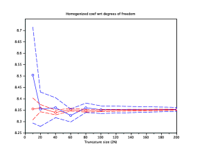
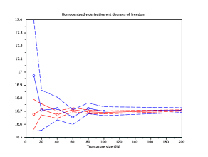
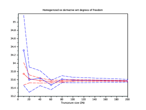
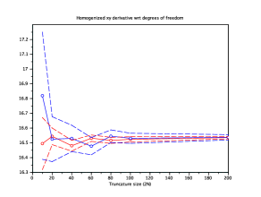
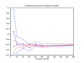
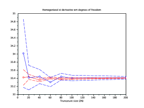
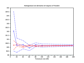
Figure 1: Test-Case 1: Homogenized quantities as a function of $N$, for the vector $\xi=(1,1)^{T}$ (Blue: Monte Carlo results; Red: Antithetic variable approach; Dashed lines: 95% confidence interval, equating the cost of the two approaches). From top left to bottom right: $\mathbb{E}\left[W^{\star}_{N}(\cdot,\xi)\right]$, $\mathbb{E}\left[\partial_{\xi_{1}}W^{\star}_{N}(\cdot,\xi)\right]$, $\mathbb{E}\left[\partial_{\xi_{2}}W^{\star}_{N}(\cdot,\xi)\right]$, $\mathbb{E}\left[\partial_{\xi_{1}\xi_{1}}W^{\star}_{N}(\cdot,\xi)\right]$, $\mathbb{E}\left[\partial_{\xi_{1}\xi_{2}}W^{\star}_{N}(\cdot,\xi)\right]$, $\mathbb{E}\left[\partial_{\xi_{2}\xi_{2}}W^{\star}_{N}(\cdot,\xi)\right]$, $\mathbb{E}\left[\xi\cdot\partial_{\xi}W^{\star}_{N}(\cdot,\xi)\right]$ and $\mathbb{E}\left[\xi^{T}\partial^{2}_{\xi}W^{\star}_{N}(\cdot,\xi)\xi\right]$.

We now turn to a more quantitative analysis of the variance. Figure 2 shows the variances

$$V_{\rm MC}=\frac{1}{2}\mathbb{V}{\rm ar}\left[W^{\star}_{N}(\cdot,\xi)\right]\quad\text{and}\quad V_{\rm AV}=\mathbb{V}{\rm ar}\left[\widetilde{W}^{\star}_{N}(\cdot,\xi)\right]$$ (56)

as a function of $N$ (note the factor $1/2$ in the definition of $V_{\rm MC}$, consistent with (12), (13) and (14)). We observe that the variance of any of our quantities of interest (obtained either with the Monte Carlo approach or the Antithetic Variable approach) decreases at the rate $1/|Q_{N}|$ as $N$ increases (as expected if one could use the Central Limit Theorem). We also observe that the variance obtained with our approach is systematically smaller than the Monte Carlo variance, in the sense that $V_{\rm AV}\leq V_{\rm MC}$.

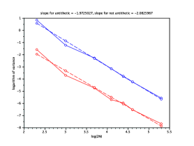
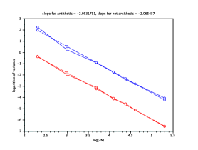
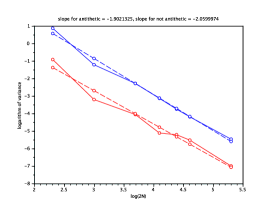
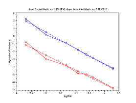
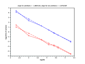
Figure 2: Test-Case 1: Variances (56) of the same quantities of interest as on Figure 1, as a function of $N$ (Blue: Monte Carlo approach; Red: Antithetic Variable approach).

We next report on Table 1 the variance reduction ratio

$$R=\frac{V_{\rm MC}}{V_{\rm AV}}=\frac{\mathbb{V}{\rm ar}\left[W^{\star}_{N}(\cdot,\xi)\right]}{2\mathbb{V}{\rm ar}\left[\widetilde{W}^{\star}_{N}(\cdot,\xi)\right]},$$ (57)

which measures the gain in computational cost at equal accuracy, or the square of the accuracy gain at equal computational cost. Although this ratio somewhat varies with $N$, we observe that it is of the order of 10 for all quantities of interest, except for $\partial_{\xi_{1}\xi_{2}}W^{\star}_{N}$, for which it is always larger than 4. In particular, even if $N$ is not large (because we cannot afford to work on a large domain $Q_{N}$), we still observe variance reduction.

$2N$	$W^{\star}_{N}$	$\partial_{\xi_{1}}W^{\star}_{N}$	$\partial_{\xi_{2}}W^{\star}_{N}$	$\partial_{\xi_{1}\xi_{1}}W^{\star}_{N}$	$\partial_{\xi_{1}\xi_{2}}W^{\star}_{N}$	$\partial_{\xi_{2}\xi_{2}}W^{\star}_{N}$	$\xi\cdot\partial_{\xi}W^{\star}_{N}$	$\xi^{T}\partial^{2}_{\xi}W^{\star}_{N}\xi$
10	19.41	11.26	13.86	9.846	5.966	13.34	19.39	19.41
20	22.82	11.89	13.03	9.865	7.306	9.096	22.77	22.83
40	18.08	11.82	9.816	9.576	5.904	8.831	18.03	18.11
60	21.26	12.89	12.98	10.57	7.247	10.73	21.24	21.28
80	12.36	8.798	9.050	10.05	4.316	8.454	12.31	12.37
100	11.88	9.856	8.412	11.10	3.775	10.24	11.82	11.88
200	13.60	8.261	11.52	8.057	4.636	12.62	13.54	13.61

Table 1: Test-Case 1: Variance reduction ratios (57).

Remark 13.

Similar variance reduction ratios are obtained in the case when the corrector problem is supplemented with homogeneous Dirichlet boundary conditions on the boundary on $Q_{N}$, rather than periodic boundary conditions as used here following (8) (results not shown).

3.4 Test Case 2

We now consider a test-case for which the energy density is not positively homogeneous. From our results of Section 2.1, we know that our approach yields variance reduction for the estimation of $\mathbb{E}\left[W^{\star}_{N}(\cdot,\xi)\right]$. Our aim here is two-fold: we first quantify the efficiency gain, and we next verify (and this will indeed be the case) that we also obtain a gain in efficiency for quantities of interest (such as the first or second derivatives of $W^{\star}_{N}(\omega,\xi)$ with respect to $\xi$) for which we do not have theoretical results in the two-dimensional case.

We show on Figure 3 the variances (56) of the same quantities of interest as previously (obtained either with the Monte Carlo approach or the Antithetic Variable approach). As for the previous test-case, we observe that all variances decrease at the rate $1/|Q_{N}|$ as $N$ increases. In addition, we observe that the variance obtained with our approach is systematically smaller than the Monte Carlo variance, in the sense that $V_{\rm AV}\leq V_{\rm MC}$.

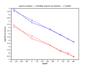
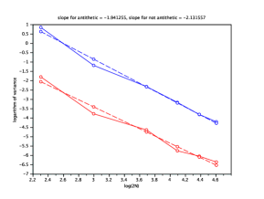
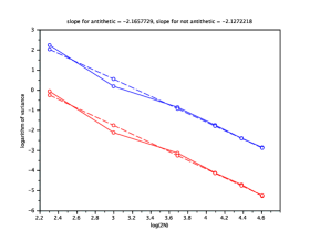
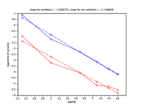
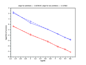
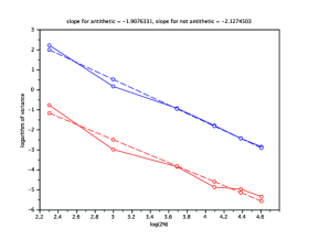
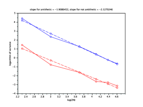
Figure 3: Test-Case 2: Variances (56) as a function of $N$ (Blue: Monte Carlo approach; Red: Antithetic Variable approach). The quantities of interest are the same as on Figure 1.

On Table 2, we report the variance reduction ratios (57) (with the same convention as in Table 1). We observe an efficiency gain of more than 10 for all quantities of interest, except again the cross derivative $\partial_{\xi_{1}\xi_{2}}W^{\star}_{N}$, for which the gain is smaller, and of the order of 4.

$2N$	$W^{\star}_{N}$	$\partial_{\xi_{1}}W^{\star}_{N}$	$\partial_{\xi_{2}}W^{\star}_{N}$	$\partial_{\xi_{1}\xi_{1}}W^{\star}_{N}$	$\partial_{\xi_{1}\xi_{2}}W^{\star}_{N}$	$\partial_{\xi_{2}\xi_{2}}W^{\star}_{N}$	$\xi\cdot\partial_{\xi}W^{\star}_{N}$	$\xi^{T}\partial^{2}_{\xi}W^{\star}_{N}\xi$
10	20.38	11.57	14.14	9.940	6.206	13.28	19.89	19.57
20	23.86	12.34	13.32	9.993	7.548	9.265	23.33	23.00
40	18.94	12.16	10.16	9.726	6.060	8.902	18.50	18.24
60	22.11	13.30	13.35	10.73	7.513	10.88	21.68	21.41
80	12.89	9.080	9.295	10.09	4.420	8.598	12.61	12.45
100	12.37	10.17	8.635	11.21	3.896	10.24	12.12	11.96

Table 2: Test-Case 2: Variance reduction ratios (57).

3.5 Test Case 3

We eventually turn to our final test-case, where both coefficients $a$ and $c$ do depend on the space variable.

We show on Figure 4 the variances (56) of our quantities of interest. Again, we observe that they all decrease at the rate $1/|Q_{N}|$ as $N$ increases, and that the variance obtained with our approach is systematically smaller than the Monte Carlo variance.

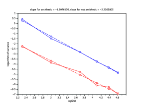
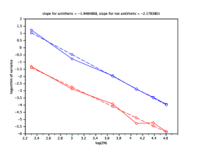
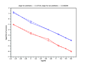
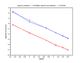
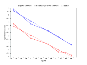
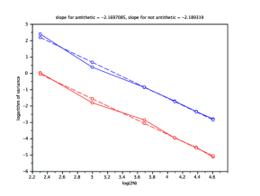
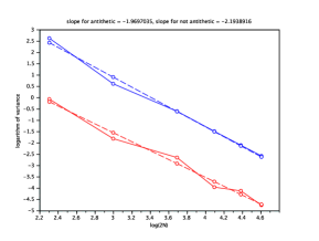
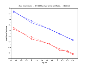
Figure 4: Test-Case 3: Variances (56) as a function of $N$ (Blue: Monte Carlo approach; Red: Antithetic Variable approach). The quantities of interest are the same as on Figure 1.

On Table 3, we report the variance reduction ratios (57) (with the same convention as in Table 1). Results are quantitatively similar to the ones obtained on Table 2: we do observe a robust variance reduction, even in cases for which theoretical support is still currently missing.

$2N$	$W^{\star}_{N}$	$\partial_{\xi_{1}}W^{\star}_{N}$	$\partial_{\xi_{2}}W^{\star}_{N}$	$\partial_{\xi_{1}\xi_{1}}W^{\star}_{N}$	$\partial_{\xi_{1}\xi_{2}}W^{\star}_{N}$	$\partial_{\xi_{2}\xi_{2}}W^{\star}_{N}$	$\xi\cdot\partial_{\xi}W^{\star}_{N}$	$\xi^{T}\partial^{2}_{\xi}W^{\star}_{N}\xi$
10	14.26	12.69	10.00	12.38	8.333	10.65	14.76	19.37
20	10.82	8.166	7.669	8.304	7.730	8.827	11.29	18.11
40	7.014	7.077	5.613	10.28	6.776	7.310	7.731	14.32
60	10.45	10.84	8.666	11.72	8.896	9.524	11.82	19.01
80	6.961	5.880	7.250	8.800	4.646	8.996	7.522	11.10
100	8.543	6.780	7.970	8.873	4.669	10.26	8.798	11.66

Table 3: Test Case 3: Variance reduction ratios (57).

References

- [1] A. Abdulle and G. Vilmart, A priori error estimates for finite element methods with numerical quadrature for nonmonotone nonlinear elliptic problems, Numer. Math., 121:397-431, 2012.
- [2] A. Anantharaman, R. Costaouec, C. Le Bris, F. Legoll and F. Thomines, Introduction to numerical stochastic homogenization and the related computational challenges: some recent developments, W. Bao and Q. Du eds., Lecture Notes Series, Institute for Mathematical Sciences, National University of Singapore, vol. 22, 197-272 (2011).
- [3] J. W. Barrett and W. B. Liu, Finite Element approximation of the p-Laplacian, Maths. of Comp., 61(204):523–537, 1993.
- [4] A. Bensoussan, J.-L. Lions and G. Papanicolaou, Asymptotic analysis for periodic structures, Studies in Mathematics and its Applications, vol. 5. North-Holland Publishing Co., Amsterdam-New York, 1978.
- [5] X. Blanc, R. Costaouec, C. Le Bris and F. Legoll, Variance reduction in stochastic homogenization: the technique of antithetic variables, in Numerical Analysis and Multiscale Computations, B. Engquist, O. Runborg and R. Tsai eds., Lect. Notes Comput. Sci. Eng., vol. 82, Springer, 47-70 (2012).
- [6] X. Blanc, R. Costaouec, C. Le Bris and F. Legoll, Variance reduction in stochastic homogenization using antithetic variables, Markov Processes and Related Fields, 18(1):31-66, 2012 (preliminary version available at http://cermics.enpc.fr/legoll/hdr/FL24.pdf).
- [7] A. Bourgeat and A. Piatnitski, Approximation of effective coefficients in stochastic homogenization, Ann I. H. Poincaré - PR, 40(2):153–165, 2004.
- [8] S.-S. Chow, Finite Element error estimates for nonlinear elliptic equations of monotone type, Numer. Math., 54:373–393, 1989.
- [9] D. Cioranescu and P. Donato, An introduction to homogenization, Oxford Lecture Series in Mathematics and its Applications, vol. 17. Oxford University Press, New York, 1999.
- [10] R. Costaouec, C. Le Bris and F. Legoll, Variance reduction in stochastic homogenization: proof of concept, using antithetic variables, Boletin Soc. Esp. Mat. Apl., 50:9–27, 2010.
- [11] G. Dal Maso and L. Modica, Nonlinear stochastic homogenization, Annali di matematica pura ed applicata, 144(4):347-389, 1986.
- [12] G. Dal Maso and L. Modica, Nonlinear stochastic homogenization and ergodic-theory, J. Reine Angewandte Mathematik, 368:28-42, 1986.
- [13] B. Engquist and P. E. Souganidis, Asymptotic and numerical homogenization, Acta Numerica, 17:147–190, 2008.
- [14] A. Gloria and S. Neukamm, Commutability of homogenization and linearization at identity in finite elasticity and applications, Ann. I. H. Poincaré - AN, 28:941–964, 2011.
- [15] A. Gloria and F. Otto, An optimal error estimate in stochastic homogenization of discrete elliptic equations, Ann. Appl. Probab., in press.
- [16] R. Glowinski and A. Marrocco, Sur l’approximation par éléments finis d’ordre un, et la résolution, par pénalisation-dualité, d’une classe de problèmes de Dirichlet non linéaires, RAIRO Anal. Numér., 2:41–76, 1975.
- [17] V. V. Jikov, S. M. Kozlov and O. A. Oleinik, Homogenization of differential operators and integral functionals, Springer-Verlag, 1994.
- [18] U. Krengel, Ergodic theorems, de Gruyter Studies in Mathematics, vol. 6, de Gruyter, 1985.
- [19] C. Le Bris, Some numerical approaches for “weakly” random homogenization, in Numerical mathematics and advanced applications, Proceedings of ENUMATH 2009, G. Kreiss, P. Lötstedt, A. Malqvist and M. Neytcheva eds., Lect. Notes Comput. Sci. Eng., Springer, 29-45 (2010).
- [20] P. Le Tallec, Numerical methods for nonlinear three-dimensional elasticity, in Handbook of numerical analysis, vol. III, P. Ciarlet and J.-L. Lions eds., North Holland, Amsterdam, 465-624 (1994).
- [21] J. S. Liu, Monte-Carlo strategies in scientific computing, Springer Series in Statistics, 2001.
- [22] A. N. Shiryaev, Probability, Graduate Texts in Mathematics, vol. 95, Springer, 1984.
- [23] L. Tartar, Estimations of homogenized coefficients, in Topics in the mathematical modelling of composite materials, A. Cherkaev and R. Kohn eds., Progress in nonlinear differential equations and their applications, vol. 31, Birkhäuser, 1987.
- [24] A. A. Tempel’man, Ergodic theorems for general dynamical systems, Trudy Moskov. Mat. Obsc., 26:94–132, 1972.
- [25] V. Thomée, Galerkin Finite Element Methods for Parabolic Problems, Springer Series in Computational Mathematics, vol. 25, 2006.