On the energy dependence of the $D^{+}/D^{-}$ production asymmetry

Abstract

In this paper we discuss the origin of the asymmetry present in $D$ meson production and its energy dependence. In particular, we have applied the meson cloud model to calculate the asymmetries in $D^{-}/D^{+}$ meson production in high energy $p-p$ collisions and find a good agreement with recent LHCb data. Although small, this non-vanishing asymmetry may shed light on the role played by the charm meson cloud of the proton.

I Introduction

It is experimentally well known DATA1 ; DATA2 ; DATA3 ; DATA4 ; WA89_99 ; selex that there is a significant difference between the $x_{F}$ (Feynman momentum) distributions of $D^{+}$ and $D^{-}$ mesons produced in hadronic collisions with proton, $\Sigma^{-}$ and pion projectiles. It is usually quantified in terms of the asymmetry function:

$$A=\frac{N_{D^{-}}-N_{D^{+}}}{N_{D^{-}}+N_{D^{+}}}$$ (1)

where $N$ may represent the number of mesons of a specific type or its distribution in $x_{F}$, rapidity $y$ and $p_{T}$. The recent data of the COMPASS collaboration compass have confirmed the existence of charm production asymmetries also in $\gamma p$ collisions. Moreover, the very recent data from the LHCb collaboration DLHCb showed that there is asymmetry in the production of $D^{+}$ and $D^{-}$ mesons in proton-proton collisions at $7$ TeV. The origin of these asymmetries is still an open question. It is not possible to understand these production asymmetries only with usual perturbative QCD (pQCD) or with the string fragmentation model contained in PYTHIA. This has motivated the construction of alternative models nnnt ; icm1 ; icm2 which were able to obtain a reasonable description of the low energy data and make concrete predictions for higher energy collisions. The LHCb data allow us, for the first time, to compare the predictions of the models with high energy data. Moreover, studying the energy dependence of production asymmetries, it may be possible to learn more about forward charm production, which undoubtedly has a non-perturbative component icm1 . In this work we update one of these models, the meson cloud model or MCM nnnt , and compare its predictions with the new LHCb data.

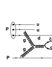
Figure 1: $D$ meson production in a proton - proton reaction. The charm pair is created by gluon fusion and then the quarks may fragment independently, as it happens to the $c$ quark in figure, or they can “recombine” or “coalesce” with one of the projectile valence quarks, as it is the case of the $\bar{c}$ in the figure. Mesons formed by recombination are harder since they are “dragged” by the hard valence quark.

Let us now briefly review some ideas about charm production. In perturbative QCD the most relevant elementary processes which are responsible for charm production are $q+\bar{q}\rightarrow c+\bar{c}$ and $g+g\rightarrow c+\bar{c}$. At high energies, due to the growth of the gluon distributions, the latter should be dominant. In standard pQCD, after being produced the $c$ and $\bar{c}$ quarks fragment independently and hence, the resulting mesons $D^{+}$ and $D^{-}$ (also $D^{0}$ and $\bar{D}^{0}$) will have the same rapidity, $p_{T}$ and $x_{F}$ distributions. This is indeed true for the bulk of charm production. Differences between the $D^{+}$ and $D^{-}$ $x_{F}$ distributions appear at large $x_{F}$, with $D^{-}$ being harder. Given the valence quark content of the proton $p(uud)$ and of the $D^{-}(d\bar{c})$, a natural explanation of the observed effect is that the $\bar{c}$ is dragged by the projectile valence $d$ quark, forming the, somewhat harder, $d\bar{c}$ bound state. This process has been usually called recombination or coalescence and it is illustrated in Fig. 1. This is a non-perturbative process and recombination models have been first proposed long time ago chiu ; hwa ; russo and then used more recently newrec ; rapp to study the accumulated experimental data and to make predictions for the RHIC collisions. Unfortunately, the current RHIC experimental set up did not allow for a precise determination of production asymmetries. However, a more detailed analysis of the heavy quark sector is expected to be possible in the upgraded RHIC facility - RHIC II rhic2 .

An alternative way to implement the idea of recombination is to use a purely hadronic picture of charm production, in which, instead of producing charm pairs and then recombining them with the valence quarks, we assume that the incoming proton fluctuates into a virtual charm meson - charm baryon pair, which may be liberated during the interaction with the target. This kind of fluctuation is unavoidable in any field theoretical description of hadrons and, in fact, it was shown ku to be quite relevant to the understanding of hadron structure. It has been also successfully applied to particle production in high energy soft hadron collisions hss ; cdnn and in nnnt it has been extended to the charm sector. This mechanism, in which the “meson cloud” plays a major role, is quite economical and can be improved systematically (see mel for light mesons). From now on we shall call it meson cloud model (MCM). A simple and accurate description of charm asymmetry production at lower energies ($\sqrt{s}\simeq 10-40$ GeV) within the framework of the MCM can be found in cdnn01 .

Another popular model of forward charm production is the intrinsic charm model (ICM) icm1 ; icm2 ; gnu . The existence of an intrinsic charm component in the wave function enhances charm meson production at large $x_{F}$. While IC, as formulated in icm1 ; icm2 is supported by several phenomenological analises, it is, alone, not enough to explain the difference between the $D^{+}$ and $D^{-}$ $x_{F}$ distributions. It is necessary to add a recombination mechanism (or “coalescence”) in this kind of model to account for the observed asymmetries. In icm1 ; icm2 the intrinsic charm component of the proton is the higher Fock state $|uudc\bar{c}\rangle$ and its existence is attributed to a multigluon fusion, which is not calculable in pQCD. In nnnt the intrinsic charm component of the proton was a consequence of the meson-baryon fluctuations mentioned above. In this approach, since they “feel” the virtual bound states where they once were, the $c$ and $\bar{c}$ distributions are different from the beginning and when they later undergo independent fragmentation their difference will be transmitted to the final $D$ mesons. Thus, in its “meson cloud” version, intrinsic charm may account for large $x_{F}$ charm meson production including the asymmetries. The charm quarks of the projectile wave function traverse the target and fragment independently. In this corner of the phase space this mechanism may be more effective than gluon fusion because the later generates final mesons with a $x_{F}$ distribution peaked at zero. This possibility was explored in gnu .

The appearance of the first LHCb data on asymmetries DLHCb opens the exciting possibility of studying the energy dependence of forward charm production. Indeed, more than ten years from the last data on this subject, we have now data taken at an energy which is larger than the previous one by a factor of $\simeq 200$ ! What do the models discussed above have to say about the energy dependence of forward charm production? What will be the fate of the production asymmetries ? The answer to this question is interesting not only to the hadron physics community but also to the studies of CP violation, since a change in the relative yield of particles and antiparticles may affect the interpretation of their decays and hence change the ammount of CP violation.

Naively, we expect that perturbative processes grow faster and become more important than non-perturbative ones as the reaction energy increases. As a consequence the asymmetries would gradually disappear. In nosco a kinematical treatment of this problem arrived at the conclusion that, as the collision energy grows, the energy deposition in the central region increases. Baryon stopping also increases, the remnant valence quarks emerge from the collision with less energy and when they recombine with charm antiquarks the outgoing charm mesons with these quarks will be decelerated and their $x_{F}$ distribution will become invisible, buried under the much higher contribution from the (symmetric) central gluon fusion. In rapp , using a recombination approach, the authors concluded that the asymmetry remains nearly constant with energy. In the meson cloud approach of cdnn01 the energy dependence of the asymmetry $A$ is approximately given by:

$$A\propto\frac{\sigma_{hp}(s)}{\sigma_{c\bar{c}}(s)}$$ (2)

where $\sigma_{hp}$ is hadron-proton cross section and $\sigma_{c\bar{c}}$ is the total $c\bar{c}$ pair production cross section, which grows faster than the hadronic cross sections. Therefore the asymmetry decreases with the energy.

In this work we use the model developed in cdnn01 to study the recent LHCb data on $D^{+}/D^{-}$ asymmetry and to check if the energy behavior of this asymmetry can be satisfactorily understood with this model. The paper is organized as follows. In the next Section, we discuss the asymmetry production in terms of the meson cloud model, presenting the main formulas and assumptions of the model. In Section III we present our results for the asymmetries in $\Lambda$ and $D$ production at SELEX ($\sqrt{s}=33$ GeV) and LHCb ($\sqrt{s}=7$ TeV) energies. We compare the results with the current data and make predictions for $\sqrt{s}=14$ TeV. Finally, in Section IV we summaryze our main conclusions.

II Asymmetry Production in the Meson Cloud Model

II.1 The interaction between the cloud and the target

In the MCM we assume that quantum fluctuations in the projectile play an important role. The proton may be decomposed in a series of Fock states, containing states such as $|p\rangle=|uud\bar{c}c\rangle$. In the MCM we write the Fock decomposition in terms of the equivalent hadronic states, such as $|p\rangle=|\Sigma_{c}^{++}D^{-}\rangle$. This expansion contains the “bare” terms (without cloud fluctuations), light states and states containing the produced charmed meson ($D$ or $D_{s}$). The latter are, of course very much suppressed but they will be responsible for asymmetries. The “bare” states occur with a higher probability and are responsible for the bulk of charm meson production at low and medium momentum ($x_{F}\leq 0.4$), including, for example the perturbative QCD contribution. The cloud states are less frequent fluctuations and contribute to $D$ production in the ways described below. More precisely we shall assume that:

$$|p\rangle=Z\,[\,|p_{0}\rangle\,+\,...\,+\,|MB\rangle\,+\,...\,+\,|\Lambda_{c}\bar{D}_{0}\rangle\,+\,|\Sigma_{c}^{++}D^{-}\rangle]$$ (3)

where $Z$ is a normalization constant, $|p_{0}\rangle$ is the “bare” proton and the “dots” denote all possible meson (M) - baryon (B) cloud states $|MB\rangle$ in the proton. The relative normalization of these states is fixed once the cloud parameters are fixed. The proton is thus regarded as being a sum of virtual meson-baryon pairs and a proton-proton reaction can thus be viewed as a reaction between the “constituent” mesons and baryons of the projectile proton with the target proton (or nucleus).

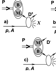
Figure 2: $pp$ collision in which the projectile is in a $|MB\rangle$ state. Figs. a) and b) show the “indirect” $D^{\pm}$ production and c) the “direct” $D^{-}$ production.

With a proton beam the possible reaction mechanisms for $D^{-}$ meson production at large $x_{F}$ and small $p_{T}$ (the soft regime) are illustrated in Fig. 2. In Fig. 2 a) the baryon just “flies through”, whereas the corresponding meson interacts inelastically producing a $D$ meson in the final state. In Fig. 2 b) the meson just “flies through”, whereas the corresponding baryon interacts inelastically producing a $D$ meson in the final state. In Fig. 2 c) the meson in the cloud is already a $D^{-}$ which escapes (similar considerations hold for $D^{-}$ production with a $\pi^{-}$ beam). This last mechanism is the main responsible for generating asymmetries. We shall refer to the first two processes as “indirect production” ($I$) and to the last one as “direct production” ($D$). The first two are calculated with convolution formulas whereas the last one is given basically by the meson momentum distribution in the initial $|MB\rangle$ cloud state. Direct production has been widely used in the context of the MCM and applied to study $n$, $\Delta^{++}$ and $\pi^{0}$ production hss . Indirect meson production has been considered previously in cdnn .

Inside the baryon, in the $|MB\rangle$ state, the meson and baryon have fractional momentum $y_{M}$ and $y_{B}$ with distributions called $f_{M/MB}(y_{M})$ and $f_{B/MB}(y_{B})$ respectively (we shall use for them the short notation $f_{M}$ and $f_{B}$). Of course, by momentum conservation, $y_{M}+y_{B}=1$ and these distributions are related by ku ; cdnn :

$$f_{M}(y)=f_{B}(1-y)$$ (4)

The “splitting function” $f_{M}(y)$ represents the probability density to find a meson with momentum fraction $y$ of the total cloud state $|MB\rangle$. With $f_{M}$ and $f_{B}$ we can compute the differential cross section for production of $D$, $\bar{D}_{0}$ and $\Lambda_{c}$. In what follows we write the formulas for the specific case of $D$ production but it is easy, with the proper replacements, to write the corresponding expressions for $\bar{D}_{0}$ and $\Lambda_{c}$. In the reaction $pp\rightarrow D^{-}X$ the differential cross section for $D$ production is given by:

$$\frac{d\sigma^{pp\rightarrow DX}}{dx_{F}}=\,\Phi_{0}\,\,+\,\,\Phi_{I}\,\,+\,\,\Phi_{D}$$ (5)

where $\Phi_{0}$ and $\Phi_{I}$ refer respectively to “bare” and indirect contributions to $D$ meson production and $x_{F}$ is the fractional longitudinal momentum of the outgoing meson. $\Phi_{D}$ represents the direct process depicted in Fig. 2 c) and is given by hss ; cdnn :

$$\Phi_{D}=\frac{\pi}{x_{F}}\,f_{D}(x_{F})\,\sigma^{\Sigma p}$$ (6)

where $f_{D}\equiv f_{D^{-}/\Sigma_{c}^{++}D^{-}}$ and $\sigma^{\Sigma p}$ is the total $p\,\Sigma_{c}^{++}$ cross section.

In the MCM the proton is from the start replaced by meson ($M$) and baryon ($B$) constituents, which interact independently with the target. In the projectile frame the $M$ and $B$ constituents can be considered as approximately free, since their interaction energy is much smaller than the energy carried by the incoming proton, which will smash $M$ or $B$ individually. This is sometimes called the impulse approximation. The subprocesses $M+\mbox{target}\rightarrow D^{\pm}+X$ and $B+\mbox{target}\rightarrow D^{\pm}+X^{\prime}$ involve different initial and final states and their amplitudes are not supposed to be added (and subsequently squared). We have rather to compute the corresponding cross sections, which we call $\sigma^{Mp}$ and $\sigma^{Bp}$, multiply them by the respective weigth, given by the function $f(y)$, and then sum the cross sections. This is why, in our case, the cross section reduces to the sum shown in Eq. (5). The splitting function $f(y)$ comes already from a squared amplitude, it is positive definite and it is interpreted as a probability ku .

Replacing $D^{\pm}$ by $\Lambda_{c}/\bar{\Lambda}_{c}$ in Figs. 2a and 2b, exchanging B with M and replacing $D^{-}$ by $\Lambda_{c}$ in Fig. 2 c) we have a pictorial representation of $\Lambda_{c}$ production in the MCM with the following expression for the direct process:

$$\Phi_{D}=\frac{\pi}{x_{F}}\,f_{\Lambda}(x_{F})\,\sigma^{Dp}$$ (7)

where $f_{\Lambda}\equiv f_{\Lambda_{c}/\Lambda_{c}\bar{D}_{0}}$ and $\sigma^{Dp}$ is the total $\bar{D}_{0}\,p$ cross section. Analogous expressions can be written for the reaction $\pi^{-}p\rightarrow DX$.

II.2 The asymmetry

Using (5), we can compute the cross sections and also the leading ($D^{-}$)/nonleading($D^{+}$) asymmetry:

$$A^{D}(x_{F}) = \frac{\frac{d\sigma^{D^{-}}(x_{F})}{dx_{F}}\,\,-\,\,\frac{d\sigma^{D^{+}}(x_{F})}{dx_{F}}}{\frac{d\sigma^{D^{-}}(x_{F})}{dx_{F}}\,\,+\,\,\frac{d\sigma^{D^{+}}(x_{F})}{dx_{F}}}$$ (8)

$$= \frac{\Phi_{D}\,\,+\,\,\Phi_{I}^{D^{-}}\,\,+\,\,\Phi_{0}^{D^{-}}\,\,-\,\,\Phi_{I}^{D^{+}}\,\,-\,\,\Phi_{0}^{D^{+}}}{\Phi_{D}\,\,+\,\,\Phi_{I}^{D^{-}}\,\,+\,\,\Phi_{0}^{D^{-}}\,\,+\,\,\Phi_{I}^{D^{+}}\,\,+\,\,\Phi_{0}^{D^{+}}}$$

$$\simeq \frac{\Phi_{D}}{\Phi_{D}\,\,+\,\,2\,\Phi_{I}^{D}\,\,+\,\,2\,\Phi_{0}^{D}}\equiv\frac{\Phi_{D}}{\Phi_{T}^{D}}$$

where the last line follows from assuming $\Phi_{I}^{D^{-}}=\Phi_{I}^{D^{+}}=\Phi_{I}^{D}$. This last assumption is made just for the sake of simplicity. In reality these contributions are not equal and their difference is an additional source of asymmetry, which we assume to be less important than $\Phi_{D}$. Since the “bare” states do not give origin to $D^{-}/D^{+}$ asymmetries (they represent mostly perturbative QCD contributions which rarely leave quark pairs in the large $x_{F}$ region), we have made use of $\Phi_{0}^{D+}=\Phi_{0}^{D-}=\Phi_{0}^{D}$. The denominator of the above expression can be replaced by a parametrization of the experimental data:

$$\Phi_{T}^{D} = \frac{d\sigma^{D^{-}}(x_{F})}{dx_{F}}\,\,+\,\,\frac{d\sigma^{D^{+}}(x_{F})}{dx_{F}}$$ (9)

$$= \sigma_{0}^{D}\,[\,(1-x_{F})^{n^{-}}\,+\,(1-x_{F})^{n^{+}}\,]$$

$$\simeq 2\,\sigma_{0}^{D}\,(1-x_{F})^{n_{D}}$$

where $n^{-}$ and $n^{+}$ are powers used by the different collaborations to fit their data. Typically $n^{+}=5$ and $n^{-}=3.5$, as suggested by the data analysis performed in DATA1 ; DATA2 ; DATA3 ; DATA4 ; WA89_99 ; selex . For the sake of simplicity we shall assume that $n^{+}=n^{-}=n_{D}=5$ for $D$ mesons. Integrating the above expression we obtain the total cross section for charged charm meson production $\sigma^{D^{\pm}}={1}/{3}\,\sigma_{0}^{D}$. Assuming isospin symmetry the charged and neutral ($\sigma^{D^{0}}$) production cross sections are equal. Neglecting the contribution of other (heavier) charm states we can relate the $D$ meson production cross section to the total $c-\bar{c}$ production cross section, $\sigma_{c\bar{c}}$, in the following way:

$$\sigma^{D^{\pm}}=\sigma^{D^{0}}=\sigma^{D}=\frac{1}{3}\sigma_{0}^{D}=\frac{1}{2}\sigma_{c\bar{c}}\,\,\,.$$ (10)

From the above relation we can extract the parameter $\sigma_{0}^{D}$ from the experimentally measured $\sigma_{c\bar{c}}$:

$$\sigma^{D}_{0}=\,1.5\,\sigma_{c\bar{c}}\,\,\,.$$ (11)

Inserting (6) and (9) into (8) the asymmetry becomes:

$$A^{D}(x_{F})=\frac{\pi\,\sigma^{\Sigma p}}{2\,\sigma_{0}^{D}}\,\,\frac{f_{D}(x_{F})}{x_{F}\,(1-x_{F})^{n_{D}}}\,\,\,.$$ (12)

An analogous development can be performed for the $\Lambda_{c}/\bar{\Lambda}_{c}$ production asymmetry, $A^{\Lambda}(x_{F})$. In the analysis made by the SELEX collaboration, the differential cross section for $\Lambda_{c}$ production was parametrized as:

$$\Phi_{T}^{\Lambda} = \frac{d\sigma^{\Lambda_{c}}(x_{F})}{dx_{F}}\,\,+\,\,\frac{d\sigma^{\bar{\Lambda}_{c}}(x_{F})}{dx_{F}}$$ (13)

$$\simeq 2\,\sigma_{0}^{\Lambda}\,(1-x_{F})^{n_{\Lambda}}$$

with $n_{\Lambda}\simeq 2$. Integrating the above expression we obtain the total cross section for $\Lambda_{c}$ and $\bar{\Lambda}_{c}$ production $\sigma^{\Lambda}={2}/{3}\,\sigma_{0}^{\Lambda}$, which, according to gavai , can be related to the total $c-\bar{c}$ production cross section, $\sigma_{c\bar{c}}$, in the following way:

$$\sigma^{\Lambda}=\frac{2}{3}\sigma_{0}^{\Lambda}\simeq 0.1\,\sigma_{c\bar{c}}$$ (14)

from where we finally have:

$$\sigma_{0}^{\Lambda}=\,0.15\,\sigma_{c\bar{c}}\,\,\,.$$ (15)

Using (4) to obtain $f_{\Lambda}$ and then inserting (7) and (13) into (8) the asymmetry $A^{\Lambda}(x_{F})$ can be written as:

$$A^{\Lambda}(x_{F})=\frac{\pi\,\sigma^{Dp}}{2\,\sigma_{0}^{\Lambda}}\,\,\frac{f_{\Lambda}(x_{F})}{x_{F}\,(1-x_{F})^{n_{\Lambda}}}$$ (16)

The behavior of (12) [ Eq. (16)] is controlled by the splitting function $f_{D}(x_{F})$ [$f_{\Lambda}(x_{F})$].

II.3 The splitting function

We now write the splitting function in the Sullivan approach ku ; cdnn . The fractional momentum distribution of a pseudoscalar meson $M$ in the state $|MB^{\prime}\rangle$ (of a baryon $|B\rangle$) is given by ku ; cdnn :

$$f_{M}(y) = \frac{g^{2}_{MBB^{\prime}}}{16\pi^{2}}\,y\int_{-\infty}^{t_{max}}dt\,\frac{[-t+(m_{B^{\prime}}-m_{B})^{2}]}{[t-m_{M}^{2}]^{2}}$$ (17)

$$\times F_{MBB^{\prime}}^{2}(t)$$

where $t$ and $m_{M}$ are the four momentum square and the mass of the meson in the cloud state and $t_{max}=m^{2}_{B}\,y-m^{2}_{B^{\prime}}\,y/(1-y)$ is the maximum $t$, with $m_{B}$ and $m_{B^{\prime}}$ respectively the $B$ and $B^{\prime}$ masses. Following a phenomenological approach, we use for the baryon-meson-baryon form factor $F_{MBB^{\prime}}$, the exponential form:

$$F_{MBB^{\prime}}(t)=\exp\left(\frac{t-m_{M}^{2}}{\Lambda^{2}_{MBB^{\prime}}}\right)$$ (18)

where $\Lambda_{MBB^{\prime}}$ is the form factor cut-off parameter. Considering the particular case where $B=p$, $B^{\prime}=\Sigma_{c}^{++}$ and $M=D^{-}$, we insert (17) into (12) to obtain the final expression for the asymmetry in our approach:

$$A^{D}(x_{F}) = \frac{N^{D}}{(1-x_{F})^{n_{D}}}$$ (19)

$$\times \int_{-\infty}^{t_{max}}dt\,\frac{[-t+(m_{\Sigma}-m_{p})^{2}]}{[t-m_{D}^{2}]^{2}}\,F_{pD\Sigma}^{2}$$

where

$$N^{D}=\frac{g^{2}_{pD\Sigma_{c}}\,\sigma^{\Sigma_{c}p}}{32\,\pi\,\sigma_{0}^{D}}$$ (20)

With the replacements $g_{pD\Sigma_{c}}\rightarrow g_{pD\Lambda_{c}}$ and $\sigma^{\Sigma_{c}p}\rightarrow\sigma^{\Lambda_{c}p}$ this same expression holds for the process $pp\rightarrow\bar{D}_{0}X$. With the replacements $g_{pD\Sigma_{c}}\rightarrow g_{pD\Lambda_{c}}$, $\sigma^{\Sigma_{c}p}\rightarrow\sigma^{Dp}$ and $\sigma_{0}^{D}\rightarrow\sigma_{0}^{\Lambda}$ the above expression holds for the process $pp\rightarrow{\Lambda}_{c}X$. For the pion beam, we need also the splitting function of the state $|\pi^{-}>\,\rightarrow\,|D^{0*}D^{-}\rangle$. In this state, the $D$ meson momentum distribution turns out to be identical to (17) except for the bracket in the numerator which takes the form $[-t+\left((m_{\pi}^{2}-m_{D^{0*}}^{2}-t)/2m_{D^{0*}}\right)^{2}]$, and for trivial changes in the definitions, i.e., $g^{2}_{MBB^{\prime}}\,\rightarrow g^{2}_{\pi DD^{0*}}$, $F_{MBB^{\prime}}\,\rightarrow F_{\pi DD^{0*}}$ and $\Lambda_{MBB^{\prime}}\,\rightarrow\,\Lambda_{\pi DD^{0*}}$. Realizing that $y=x_{F}$ in the above equations, we can see that in the limit $x_{F}\rightarrow 1$,   $t_{max}\rightarrow-\infty$ and the integral in (19) goes to zero. In fact, it vanishes faster than the denominator and therefore $A\rightarrow 0$. This behavior does not depend on the cut-off parameter but it depends on the choice of the form factor. For a monopole form factor we may obtain asymmetries which grow even at very large $x_{F}$.

To conclude this section we would like to point out that our calculation is based on quite general and well established ideas, namely that hadron projectiles fluctuate into hadron-hadron (cloud) states and that these states interact with the target. During the derivation of the expressions for the asymmetry many strong assumption have been made. In the end our results depend on two parameters: $\Lambda$ and $N$. Whereas $\Lambda$ affects the width and position of the maximum of the momentum distribution of the leading meson in the cloud (and consequently of the asymmetry), $N$ is a multiplicative factor which determines the strength of the asymmetry.

III Results and discussion

III.1 The energy dependence

Although the recent data DLHCb are given in terms of the pseudo-rapidity $\eta$, in order to study the energy dependence it is more convenient to use the Feynman $x_{F}$ variable, which may be written as:

$$x_{F}=\frac{2\,m_{T}\,cosh(y)}{\sqrt{s}}\simeq\frac{2\,m_{T}\,cosh(\eta)}{\sqrt{s}}\simeq\frac{2\,m_{T}\,e^{\eta}}{\sqrt{s}}$$

for $\eta>1$. Moreover, if the transverse momentum of the final $D$ meson is zero or very small, then $m_{T}\simeq m_{D}$.

In order to study the energy dependence of the asymmetry, we shall focus on the two energies where we have experimental data: $\sqrt{s_{1}}=33$ GeV and $\sqrt{s_{2}}=7000$ GeV and construct the asymmetry ratio:

$$R_{A}\equiv\frac{A(\sqrt{s_{2}})}{A(\sqrt{s_{1}})}=\frac{\Phi_{D}(\sqrt{s_{2}})/\Phi_{T}(\sqrt{s_{2}})}{\Phi_{D}(\sqrt{s_{1}})/\Phi_{T}(\sqrt{s_{1}})}\,\,\,.$$ (21)

Using the definitions of the splitting function (17) in (6) and then in (8), many energy independent factors cancel out and we find:

$$R_{A} = \frac{A(s_{2})}{A(s_{1})}=\left(\frac{\sigma^{\Sigma}(s_{2})}{\sigma^{\Sigma}(s_{1})}\right)/\left(\frac{\sigma_{0}^{D}(s_{2})}{\sigma_{0}^{D}(s_{1})}\right)$$ (22)

$$= \left(\frac{\sigma^{pp}(s_{2})}{\sigma^{pp}(s_{1})}\right)/\left(\frac{\sigma_{c\bar{c}}(s_{2})}{\sigma_{c\bar{c}}(s_{1})}\right)$$

where in the last step we have used (11) and assumed that $\sigma^{\Sigma}=\sigma^{\Sigma^{++}_{c}\,p}=\mbox{const}\,.\,\sigma^{p\,p}$. Moreover, we have neglected the energy dependence of $n_{D}$. The above ratios can be estimated with the recently obtained experimental data listed in Table 1.

Energy (GeV)	$\sigma_{pp}$ (mb)	$\sigma_{c\bar{c}}$ (mb)
33	40	0.04
7000	97	8
14000	110	11

Table 1: Total $pp$ cross section from fag and total $c\bar{c}$ production cross section from ram as a function of the energy. The first two lines refer to measurements and the last one show model calculations described in the corresponding references.

With these numbers we find that increasing the energy from $\sqrt{s}=33$ GeV to $7000$ GeV the asymmetry ratio is $R_{A}=1/75$, i.e., there is a strong decrease in the asymmetry. This happens because meson emission (which ultimately causes the asymmetry) is a non-perturbative process and has a slowly growing cross section. In contrast, the symmetric processes are driven by the perturbative partonic interactions, which have strongly growing cross sections. We end this subsection making the prediction for the order of magnitude of the $D^{+}/D^{-}$ asymmetry in the forthcoming $14$ TeV $pp$ collisions. Using the last line of Table 1, setting $\sqrt{s_{2}}=14$ TeV and susbtituting the numbers in (22) we find $R_{A}=1/100$ showing the decreasing trend of the asymmetry.

III.2 Predictions for the asymmetries

Due to the lack of experimental data a direct comparison of $D^{+}/D^{-}$ asymmetries in the same reaction, e.g. proton-proton, at different energies is difficult. However, we can relate and compare similar reactions.

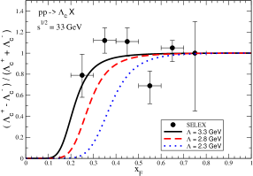
Figure 3: Comparison of the MCM asymmetry for $\Lambda_{c}$ production with experimental data selex for $\sqrt{s}=33$ GeV.

In what follows we shall relate the two sets of data on asymmetries in proton-proton collisions: the low energy one taken by the SELEX collaboration selex and the high energy one obtained by the LHCb collaboration DLHCb . We will fit the data on $\Lambda_{c}/\bar{\Lambda}_{c}$ asymmetry. This will fix the value of $N^{\Lambda}$ and define a range of possible values for the cut off $\Lambda_{\bar{D}_{0}p\Lambda_{c}}$. Using experimental information it is easy to go from the estimate of $N^{\Lambda}$ to the estimate of $N^{D}$ and then it is straightforward to calculate the associate asymmetry in $\bar{D}_{0}/D_{0}$. In proton-proton collisions the leading charm mesons are those with valence quarks and hence $\bar{D}_{0}(u\bar{c})$ has the same properties as $D^{-}(d\bar{c})$. From this approximate equivalence we infer the $D^{-}/D^{+}$ asymmetry at the lower energy. The final step is to calculate this asymmetry at the LHC energy. This extrapolation can be done, since the model has a well defined energy dependence and fortunately the necessary ingredients (the cross sections) are already available.

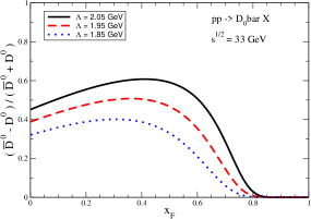
Figure 4: MCM prediction of the $\bar{D}^{0}/D^{0}$ asymmetry, Eq. (19).

III.2.1 The coupling constants

The coupling constant $g_{pD\Lambda_{c}}$ was estimated in several works with QCD sum rules gndl . Here we have chosen a representative number. In our analysis we will also need the coupling $g_{pD^{-}\Sigma^{++}_{c}}$, about which, to the best of our knowledge, nothing is known. As a first guess we will then assume that

$$g_{pD^{-}\Sigma^{++}_{c}}=g_{p\bar{D}_{0}\Lambda_{c}}=5.6\,\,\,.$$ (23)

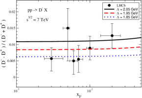
Figure 5: Comparison of the MCM asymmetry, Eq. (19), with experiental data DLHCb for $D^{-}/D^{+}$.

III.2.2 The interaction cross sections of the cloud particles

The $D$ - proton and $\Lambda_{c}$ - proton total cross sections in the $10-40$ GeV range are unknown. We know that the presence of the heavy quark makes these states much more compact than the proton and hence with smaller geometrical cross section. In the well studied case of the $J/\psi$ - proton cross section, a series of theoretical works gradually converged to $\sigma^{J/\psi p}\simeq 4$ mb noscross . Moreover, it was found that, in contrast to the expectation of additive quark models, $\sigma^{J/\psi p}\simeq\sigma^{J/\psi\pi}$. Inspired by these previous works we shall assume that:

$$\sigma^{Dp}\simeq\sigma^{\Lambda_{c}p}=0.15\,\sigma^{pp}=6\,\mbox{mb}\,\,\,.$$ (24)

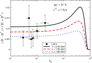
Figure 6: Comparison of the MCM asymmetry, Eq. (19), with experimental data DLHCb for $D^{-}/D^{+}$. Extension of Fig. 5 to the large $x_{F}$ region.

III.2.3 The production cross sections of the charm particles

The production cross section of charmed hadrons is measured in some cases and calculated with pQCD in others. In order to have an estimate of these cross sections it is enough for our present purposes to use the pQCD results published in gavai , from where we have deduced (11) and (15). All this information is summarized in Table 2.

$g_{pD\Lambda_{c}}$	$\sigma^{Dp}$	$\sigma^{\Lambda}_{0}$	$\sigma^{\Lambda_{c}p}$	$\sigma^{D}_{0}$
$5.6$	$0.15$ $\sigma^{pp}$	$0.15$ $\sigma_{c\bar{c}}$	$0.15$ $\sigma^{pp}$	$1.5$ $\sigma_{c\bar{c}}$

Table 2: Parameters used to calculate $N$ at $\sqrt{s}=33$ GeV.

Starting from the definition (20) and using the numbers given in Table 2 we have:

$$N^{\Lambda}=\frac{g^{2}_{pD\Lambda_{c}}}{32\,\pi}\frac{\sigma^{Dp}}{\sigma_{0}^{\Lambda}}=\frac{(5.6)^{2}}{32\,\pi}\frac{0.15\,\sigma^{pp}}{0.15\,\sigma_{c\bar{c}}}\simeq 320$$ (25)

and also:

$$N^{D}=\frac{g^{2}_{pD\Lambda_{c}}}{32\,\pi}\frac{\sigma^{\Lambda_{c}p}}{\sigma_{0}^{D}}=\frac{(5.6)^{2}}{32\,\pi}\frac{0.15\,\sigma^{pp}}{1.5\,\sigma_{c\bar{c}}}\simeq 32$$ (26)

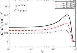
Figure 7: Prediction of the $D^{-}/D^{+}$ asymmetry for $\sqrt{s}=14$ TeV.

In Fig. 3, we show the $\Lambda_{c}/\bar{\Lambda_{c}}$ asymmetry in $pp$ collisions at $\sqrt{s}=33$ GeV. The experimental points are the results obtained by the SELEX collaboration. The lines are calculated with Eq. (16 ) with the normalization fixed by (25). These data can not impose a stringent contraint on the model, but they can establish a range of acceptable values for the cut-off parameter, which values are shown in the figure. The outcoming numbers for $\Lambda$ are those expected in this kind of meson cloud calculation. If they had been smaller than $1$ GeV or larger than $5$, this would have been an evidence against the model.

In Fig. 4, we show the $\bar{D_{0}}/D_{0}$ asymmetry in $pp$ collisions at $\sqrt{s}=33$ GeV. It was calculated with Eq. (19) with the normalization factor given by (26). Since $N^{D}$ is fixed the only free parameter is the cut-off $\Lambda$, which, as it will be seen next, will be fixed so as to yield a good fit of the $D^{+}/D^{-}$ asymmetry data from the LHCb collaboration. Also in this case, the values of $\Lambda$ used to draw the curves are quite reasonable. The shapes of Figs. 3 and 4 are correlated since they refer to the same vertex, where the proton splitts into a meson $\bar{D}_{0}$ and a baryon $\Lambda_{c}$. Due to its larger mass the baryon takes most of the momentum and the resulting asymmetry peaks at very large values of $x_{F}$. Complementarily, the $\bar{D}_{0}$ distribution peaks at lower values of $x_{F}$, which, nevertheless, are still large. The value of the cut-off $\Lambda$ does not have to be the same as that used in Fig. 3 because, even though the coupling constant of a given vertex is always the same, the functional form of the form factor (as a function of the off-shell particle squared momentum) changes when the off-shell particle changes.

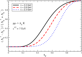
Figure 8: Prediction of the $\Lambda_{c}/\bar{\Lambda}_{c}$ asymmetry for $\sqrt{s}=7$ TeV.

Neglecting differences coming from the different isospin, we assume that, apart from trivial changes in the masses, the vertex $p\Sigma_{c}^{++}D^{-}$ has the same splitting function as the previously discussed $p\Lambda_{c}\bar{D}_{0}$ vertex and therefore the asymmetry of $D^{-}$ production is given by the same expression used for the $\bar{D}_{0}$. Now we try to reproduce the $\sqrt{s}=7$ TeV LHCb data with Eq. (19). The only part of this expression which depends on the energy is the factor $N^{D}$, which at higher energies will be corrected by the factor (22):

$$N^{D}(\sqrt{s}=7\,\mbox{TeV}) = R_{A}\,.\,N^{D}(\sqrt{s}=33\,\mbox{GeV})$$ (27)

$$= \frac{1}{75}\,N^{D}(\sqrt{s}=33\,\mbox{GeV})$$

In Fig. 5 we show Eq. (19) with $N^{D}(\sqrt{s}=7\,\mbox{TeV})$ and compare with the data, properly rewritten in terms of $x_{F}$ and with the definition (8), which introduces a minus sign with respect to DLHCb . In spite of the large error bars we can see that the MCM is able to reproduce the non-vanishing asymmetry. The data are surprisingly sensitive to cut-off choices, being able to discriminate small variations in $\Lambda$. These data can not yet give a detailed information about the $x_{F}$ dependence of the asymmetry, but they show clearly that this asymmetry exists and also that it is much smaller than what we expect to find at lower energies for $pp$ and than what we have already found for pion and $\Sigma$ projectiles. After this close look into the data points, this figure deserves a zoom out to reach the $x_{F}$ region which was scanned in previous lower energies experiments. This is shown in Fig. 6, from where we draw the most important conclusion of this work: the asymmetry definitely decreases at increasing energies, reaching at most 2 % at $x_{F}\simeq 0.4$. Finally, in Fig. 7 we show our prediction for the asymmetry to be measured at $\sqrt{s}=14$ TeV. For completeness, we present in Fig. 8 our predictions for the $\Lambda_{c}$ asymmetry at $\sqrt{s}=7$ TeV.

IV Summary

In this paper we have shown that the MCM provides a good understanding of the charm production asymmetries in terms of a simple physical picture with few parameters. It connects the behavior of the asymmetries at large $x_{F}$ with the charm meson momentum distribution within the cloud state. We can explain why we observe asymmetries, why they are different for different beams and why they decrease with increasing energies.

- (1) M. I. Adamovich et al., (WA82 Collab.), Phys. Lett. B 306, 402 (1993).
- (2) G. A. Alves et al., (E769 Collab.), Phys. Rev. Lett. 77, 2392 (1996).
- (3) E. M. Aitala et al., (E791 Collab.), Phys. Lett. B 411, 230 (1997).
- (4) M. I. Adamovich et al., (WA92 Collab.), Nucl. Phys. B 495, 3 (1997).
- (5) M. I. Adamovich et al., (WA89 Collab.), Eur. Phys. J. C 8, 593 (1999); C 13, 247 (2000).
- (6) F.G. Garcia et al. (SELEX Collab.) Phys. Lett. B 528, 49 (2002); M. Iori et al., (SELEX Collab.), Nucl. Phys. B (Proc. Suppl.) 75 , 16 (1999); hep-ex/0009049; J.C. Anjos and E. Cuautle, hep-ph/0005057.
- (7) C. Adolph et al. [COMPASS Collaboration], arXiv:1211.1575 [hep-ex].
- (8) R. Aaij et al. [LHCb Collaboration], Phys. Lett. B. 718, 902 (2013) [arXiv:1210.4112 [hep-ex]].
- (9) F. S. Navarra, M. Nielsen, C. A. A. Nunes and M. Teixeira, Phys. Rev. D 54, 842 (1996); S. Paiva, M. Nielsen, F. S. Navarra, F. O. Durães and L. L. Barz, Mod. Phys. Lett. A 13, 2715 (1998); W. Melnitchouk and A.W. Thomas, Phys. Lett. B 414, 134 (1997).
- (10) S. J. Brodsky, P. Hoyer, C. Peterson and N. Sakai, Phys. Lett. B 93, 451 (1980).
- (11) R. Vogt, S. J. Brodsky and P. Hoyer, Nucl. Phys. B 360, 67 (1991); R. Vogt and S. J. Brodsky, Nucl. Phys. B 438, 261 (1995); Nucl. Phys. B 478, 311 (1996).
- (12) K.P. Das et al., Phys. Lett. B 68, 459 (1977); Erratum-ibid. B 73, 504 (1978); C.B. Chiu et al., Phys. Rev. D 20, 211 (1979).
- (13) R. Hwa, Phys. Rev. D 22, 1593 (1980).
- (14) V.G. Kartvelishvili et al., Sov. J. Nucl. Phys. 33, 434 (1981); A.K. Likhoded et al., Sov. J. Nucl. Phys. 38, 433 (1983).
- (15) E. Cuautle et al., Eur. Phys. J. C 2, 473 (1998); E. Braaten et al., Phys. Rev. Lett. 89, 122002 (2002); T. Mehen, J. Phys. G 30, S295 (2004); C. Avila, J. Magnin and L. M. Mendoza-Navas, hep-ph/0307358.
- (16) R. Rapp and E. V. Shuryak, Phys. Rev. D 67, 074036 (2003).
- (17) A. D. Frawley, T. Ullrich and R. Vogt, Phys. Rept. 462, 125 (2008)
- (18) for a review see J. Speth and A. W. Thomas, Adv. Nucl. Phys. 24, 83 (1998); S. Kumano, Phys. Rep. 303, 183 (1998); A.W. Thomas, Phys. Lett. B 126, 97 (1983).
- (19) H. Holtmann, A. Szczurek and J. Speth, Nucl. Phys. A 569, 631 (1996); N. N. Nikolaev, W. Schaefer, A. Szczurek and J. Speth, Phys. Rev. D 60, 014004 (1999).
- (20) F. Carvalho, F. O. Durães, F. S. Navarra and M. Nielsen, Phys. Rev. D 60, 094015 (1999); F. S. Navarra, M. Nielsen and S. Paiva, Phys. Rev. D 56, 3041 (1997).
- (21) M. Burkardt, K. S. Hendricks, C. -R. Ji, W. Melnitchouk and A. W. Thomas, Phys. Rev. D 87, 056009 (2013).
- (22) F. Carvalho, F. O. Duraes, F. S. Navarra and M. Nielsen, Phys. Rev. Lett. 86, 5434 (2001).
- (23) V. P. Goncalves, F. S. Navarra and T. Ullrich, Nucl. Phys. A 842, 59 (2010).
- (24) F. O. Durães, F. S. Navarra, C. A. A. Nunes and G. Wilk, Phys. Rev. D 53, 6136 (1996).
- (25) R. V. Gavai, S. Gupta, P. L. McGaughey, E. Quack, P. V. Ruuskanen, R. Vogt and X. -N. Wang, Int. J. Mod. Phys. A 10, 2999 (1995).
- (26) D. A. Fagundes, M. J. Menon and P. V. R. G. Silva, arXiv:1208.3456 [hep-ph].
- (27) R. E. Nelson, R. Vogt and A. D. Frawley, Phys. Rev. C 87 014908 (2013).
- (28) F. S. Navarra and M. Nielsen, Phys. Lett. B 443, 285 (1998); F. O. Duraes, F. S. Navarra and M. Nielsen, Phys. Lett. B 498, 169 (2001) and references therein.
- (29) H. G. Dosch, F. S. Navarra, M. Nielsen and M. Rueter, Phys. Lett. B 466, 363 (1999); F. O. Duraes, S. H. Lee, F. S. Navarra and M. Nielsen, Phys. Lett. B 564, 97 (2003).