Efficient classical density-functional theories of rigid-molecular fluids and a simplified free energy functional for liquid water

Abstract

Classical density-functional theory provides an efficient alternative to molecular dynamics simulations for understanding the equilibrium properties of inhomogeneous fluids. However, application of density-functional theory to multi-site molecular fluids has so far been limited by complications due to the implicit molecular geometry constraints on the site densities, whose resolution typically requires expensive Monte Carlo methods. Here, we present a general scheme of circumventing this so-called inversion problem: compressed representations of the orientation density. This approach allows us to combine the superior iterative convergence properties of multipole representations of the fluid configuration with the improved accuracy of site-density functionals. Next, from a computational perspective, we show how to extend the DFT++ algebraic formulation of electronic density-functional theory to the classical fluid case and present a basis-independent discretization of our formulation for molecular classical density-functional theory. Finally, armed with the above general framework, we construct a simplified free-energy functional for water which captures the radial distributions, cavitation energies, and the linear and non-linear dielectric response of liquid water. The resulting approach will enable efficient and reliable first-principles studies of atomic-scale processes in contact with solution or other liquid environments.

1 Introduction

The microscopic structure of liquids plays an important role in several biological processes and chemical systems of technological importance, and is the subject of continued scientific interest. Several computational techniques have been developed to study the bulk and inhomogeneous properties of liquids. (See [1] for a comprehensive review.)

Monte Carlo calculations and molecular dynamics simulations with a simplified Hamiltonian, often composed of additive pair-potentials, are the most popular techniques used to compute properties of inhomogeneous liquids. However these can be quite expensive due to the long equilibration times and extensive phase-space sampling necessary to compute thermodynamic averages with sufficiently low statistical noise.

Theories in terms of the equilibrium densities rather than individual configurations of molecules avoid this phase space sampling and hence are much more efficient for the computation of equilibrium properties. Integral equation theories, based on approximations to the diagrammatic series of interactions, can be reasonably accurate but still prove relatively expensive and have only recently been applied to inhomogeneous systems in three dimensions [2].

All of the above methods require the construction of a simplified Hamiltonian, usually restricted to pair potentials. Many applications, such as the determination of chemical reaction pathways, also require estimation of free energies, which involves a coupling constant integration and hence incurs additional costs. Classical density-functional theories based on an exact variational theorem for the free energy of a liquid [3] avoid these restrictions, at least in principle. In practice, they involve directly approximating the free energy as a functional of the liquid density. They have the further advantage of being readily coupled to a quantum mechanical calculation of an electronic system within the framework of joint density-functional theory [4], which makes quantum treatment practical for much larger systems than possible with ab initio molecular dynamics [5].

Free-energy functional approximations for fluids of spherical particles often employ a thermodynamic perturbation about the hard sphere fluid described accurately by fundamental measure theory [6, 7]. These may be extended to model polar fluids such as the Stockmeyer fluid [8], but the accuracy of such theories for real molecular fluids is not satisfactory.

Molecular fluids are best described within the reduced interaction-site models (RISM) [9], which express the interactions in terms of a few sites on each molecule, usually on atomic centers constrained by a rigid model molecular geometry. The free energy functional descriptions in terms of these site densities, however, is complicated by the molecular geometry constraints; even the ideal-gas free-energy is no longer expressible as an analytical closed-form functional of the site-densities alone. An explicit functional can be written by introducing effective ideal-gas site potentials as auxiliary variables [10], but this still requires inversion of an integral equation to obtain these potentials from the site densities, a problem which can be solved explicitly only in some limits such as reducing the molecule to a point [11], and requires an expensive Monte Carlo integration for the general case.

The above inversion problem can effectively be avoided [12] by switching to the site potentials as the independent variables instead of the site densities. This method was applied successfully to fluids of hydrogen chloride [12] and water [13] in one dimension. The convergence of free energy minimization with respect to these independent variables turns out to be quite slow, however, particularly in the presence of strong electric fields.

This work presents a simple general scheme of choosing independent variables that can generate the site densities for the free-energy functional treatment of molecular fluids. In Section 2, we demonstrate the site-potential solution as a special case of this general scheme and present other representations with better iterative convergence during free energy minimization. In section 3, we construct a simplified semi-empirical excess functional for liquid water which adequately captures the properties most critical to successful ab initio treatment of solvation within the framework of joint density-functional theory. Finally in section 4, we detail the computational implementation of the above theories in the open-source plane-wave density-functional theory software JDFTx [14], using the basis-independent DFT++ algebraic formulation [15], and present numerical studies of the molecular classical density-functional framework and the free energy functional for liquid water.

2 Free energy of an ideal gas of rigid molecules

The site-density-functional theory of molecular fluids is based on functional approximations to the in-principle exact free-energy functional

$$\Phi[\{N_{\alpha}(\vec{r})\}]=\Phi_{\textrm{id}}[\{N_{\alpha}\}]+F_{\textrm{ex}}[\{N_{\alpha}\}],$$ (1)

where $\Phi$ is the grand free energy of the interacting fluid, $\Phi_{\textrm{id}}$ is the exact grand free energy for the molecular ideal gas, $N_{\alpha}(\vec{r})$ are the densities of distinct sites (indexed by $\alpha$) in the molecule, and $F_{\textrm{ex}}$ captures the effect of all the interactions and correlations. The equilibrium densities and free energy are obtained by minimizing the free energy over all allowed densities.

The heart of the inversion problem lies in the fact that the site densities $N_{\alpha}(\vec{r})$ are not independent variables, but are constrained by the assumption of a rigid-molecular geometry. For definiteness, let the molecule geometry be specified by $\vec{R}_{\alpha k}$, the positions of the sites for a molecule centered at the origin in some reference orientation. Here, $\alpha$ indexes distinct sites while $k$ indexes multiple sites of the same type equivalent under the symmetry of the molecule (e.g. for a 3-site water model, $\alpha\in\{O,H\}$, $k=1$ for $\alpha=O$ and $k\in\{1,2\}$ for $\alpha=H$.)

2.1 Treatment of site-density constraints

The inversion problem in the original approach of [10, 11], which includes ideal-gas effective potentials $\psi_{\alpha}(\vec{r})$ as auxiliary independent variables in addition to the site densities, is avoided in [12] by switching to $\psi_{\alpha}(\vec{r})$ as the sole independent variables. The site densities and ideal-gas free energy in the presence of external site potentials $V_{\alpha}$ and chemical potentials $\mu_{\alpha}$ are then expressed in terms of the $\psi_{\alpha}(\vec{r})$ using

$$\Phi_{\textrm{id}}[\{\psi_{\alpha}(\vec{r})\}] =\Omega^{(ni)}[\{\psi_{\alpha}\}]+\sum_{\alpha}\int\textrm{d}\vec{r}N_{\alpha}(\vec{r})(V_{\alpha}(\vec{r})-\mu_{\alpha}-\psi_{\alpha}(\vec{r}))$$ (2)

$$\Omega^{(ni)} \equiv-N_{\textrm{ref}}T\int\prod_{\alpha,k}e^{-\psi_{\alpha}(\vec{r}_{\alpha k})/T}\textrm{d}\vec{r}_{\alpha k}s(\{\vec{r}_{\alpha k}\})$$ (3)

$$N_{\alpha}(\vec{r}) \equiv\frac{\delta\Omega^{(ni)}}{\delta\psi_{\alpha}(\vec{r})},$$ (4)

Here, the reference density $N_{\textrm{ref}}$ sets the zero of chemical potential and the constraint function $s(\{\vec{r}_{\alpha k}\})$ picks out configurations $\{\vec{r}_{\alpha k}\}$ which satisfy the rigid molecule geometry (i.e. equivalent to $\{\vec{R}_{\alpha k}\}$ under rotations and translations).

Employing a spherical harmonic expansion of the constraint function, [12] and [13] specialize (3) for diatomic and triatomic molecules respectively. However, that expansion also becomes computationally challenging as one moves to calculations without planar symmetry. Instead, we transform (3) to

$$\Omega^{(ni)}=-N_{\textrm{ref}}T\int\frac{\textrm{d}\vec{r}\textrm{d}\omega}{8\pi^{2}}\prod_{\alpha,k}e^{-\psi_{\alpha}(\vec{r}+\omega\circ\vec{R}_{\alpha k})/T}$$ (5)

where $\omega\in SO(3)$ is a rotation and $\omega\circ\vec{R}$ is the result of rotating vector $\vec{R}$ by $\omega$, and we directly discretize the integral over orientations as described in A for practical calculations in three dimensions.

It is instructive to further transform the above equations to

$$\Phi_{\textrm{id}} =T\int\frac{\textrm{d}\vec{r}\textrm{d}\omega}{8\pi^{2}}p_{\omega}(\vec{r})\left(\log\frac{p_{\omega}(\vec{r})}{N_{\textrm{ref}}}-1\right)+\sum_{\alpha}\int\textrm{d}\vec{r}N_{\alpha}(\vec{r})(V_{\alpha}(\vec{r})-\mu_{\alpha})$$ (6)

$$N_{\alpha}(\vec{r}) =\sum_{k}\int\frac{\textrm{d}\omega}{8\pi^{2}}p_{\omega}\left(\vec{r}-\omega\circ\vec{R}_{\alpha k}\right)$$ (7)

with

$$p_{\omega}(\vec{r})=N_{\textrm{ref}}\prod_{\alpha,k}e^{-\psi_{\alpha}(\vec{r}+\omega\circ\vec{R}_{\alpha k})/T}.$$ (8)

Here, $p_{\omega}(\vec{r})$ represents the probability of finding a molecule centered at location $\vec{r}$ with orientation $\omega$. For an ideal molecular gas, $p_{\omega}(\vec{r})$ is simply a product of Boltzmann factors for each site given that $\psi_{\alpha}(\vec{r})$ are ideal-gas effective potentials since they equal $V_{\alpha}(\vec{r})-\mu_{\alpha}$ when $\Phi_{\textrm{id}}$ is minimized.

Note that, given the explicit expressions for the ideal-gas free energy (6) and site densities (7), $p_{\omega}(\vec{r})$ is a natural choice for the independent variables for unconstrained free-energy minimization. Section 4.2 demonstrates that conjugate gradients minimization over $p_{\omega}(\vec{r})$ as the independent variables converges much faster than minimization over the $\{\psi_{\alpha}(\vec{r})\}$. A potential disadvantage of using $p_{\omega}(\vec{r})$ is the increased memory requirement, but practical calculations of reasonable size are possible using the efficient orientation quadratures of A. Moreover the superior convergence properties can be retained, while mitigating the memory requirements, by switching to compressed multipole representations of $p_{\omega}(\vec{r})$, as we now discuss.

2.2 Representations of the Orientation Density

Our first task in this development is to demonstrate that minimizing free energy functionals over $p_{\omega}(\vec{r})$ yields the same results as minimizing over $\{\psi_{\alpha}(\vec{r})\}$. To demonstrate this we employ a constrained search procedure, to find

$$\Phi =\min_{p_{\omega}(\vec{r})}\left(\Phi_{\textrm{id}}[p_{\omega}(\vec{r})]+F_{\textrm{ex}}[\{N_{\alpha}\}]\right)$$

$$=\min_{p_{\omega}(\vec{r})}\bigg{(}T\underbrace{\int\frac{\textrm{d}\vec{r}\textrm{d}\omega}{8\pi^{2}}p_{\omega}(\vec{r})\log\frac{p_{\omega}(\vec{r})}{N_{\textrm{ref}}}}_{-S_{\textrm{id}}[p_{\omega}(\vec{r})]}+F_{\textrm{id-ex}}[\{N_{\alpha}\}]\bigg{)},$$

which follows because all the terms in $\Phi_{\textrm{id}}$ are explicit site-density functionals except for the molecular ideal gas entropy ($S_{\textrm{id}}$) contribution separated out above. Next, the minimization over all $p_{\omega}(\vec{r})$ can be performed by minimizing over those $p_{\omega}(\vec{r})$ that yield a specific set of site densities $\{N_{\alpha}(\vec{r})\}$, and then minimizing over all $\{N_{\alpha}(\vec{r})\}$,

$$\Phi =\min_{\{N_{\alpha}(\vec{r})\}}\left(\min_{p_{\omega}(\vec{r})\mapsto\{N_{\alpha}(\vec{r})\}}T\int\frac{\textrm{d}\vec{r}\textrm{d}\omega}{8\pi^{2}}p_{\omega}(\vec{r})\log\frac{p_{\omega}(\vec{r})}{N_{\textrm{ref}}}+F_{\textrm{id-ex}}[\{N_{\alpha}\}]\right).$$

Finally, the inner, constrained minimization over $p_{\omega}(\vec{r})$ that lead to given site densities can be performed explicitly by introducing Lagrange multipliers $\psi_{\alpha}(\vec{r})$ for each $N_{\alpha}(\vec{r})$ constraint. It is straightforward to verify that the Euler-Lagrange equation for that extremization is precisely (8), so that the result of free energy minimization over $p_{\omega}(\vec{r})$ is exactly the same as the ideal-gas effective potential methods of [10, 12].

To generalize this approach, we note that the exact equivalence between minimization over $p_{\omega}(\vec{r})$ and minimization over $\{\psi_{\alpha}(\vec{r})\}$ holds only when the external potential takes the form of external site potentials $V_{\alpha}(\vec{r})$. In principle, we could go beyond the reduced-interaction site model and consider arbitrary orientation dependent external potentials $V_{\omega}(\vec{r})$ (of which site potentials $V_{\alpha}(\vec{r})$ are a special case). From this perspective, the minimization over $\{\psi_{\alpha}(\vec{r})\}$ can be reinterpreted as a minimization over only those $p_{\omega}(\vec{r})$ that maximize the molecular ideal gas entropy $S_{\textrm{id}}[p_{\omega}(\vec{r})]$ subject to site-density constraints $\{N_{\alpha}(\vec{r})\}$ (whose Lagrange-multiplier constraints become the site potentials.) The variational principle implies that this procedure will always result in a free-energy greater than or equal to direct, unconstrained minimization over $p_{\omega}(\vec{r})$, with equality guaranteed only when the external orientation potential $V_{\omega}(\vec{r})$ can be reduced to site potentials $V_{\alpha}(\vec{r})$.

These considerations lead to the perspective of the $\{\psi_{\alpha}(\vec{r})\}$ as a compressed representation of $p_{\omega}(\vec{r})$, with decompression carried out by maximizing the entropy subject to constraints for which the $\{\psi_{\alpha}(\vec{r})\}$ are Lagrange multipliers. From the most general perspective, then, any set of functional constraints $\{X_{i}=\hat{X}_{i}[p_{\omega}(\vec{r})]\}$ corresponds to a maximum-entropy compressed representation of $p_{\omega}(\vec{r})$, where the independent variables $\chi_{i}$ for the free-energy functional minimization are the Lagrange multipliers for the corresponding $X_{i}$ constraint in the maximization of $S_{\textrm{id}}[p_{\omega}(\vec{r})]$. Specifically,

$$\Phi=\min_{\{\chi_{i}\}}\left(\Phi_{\textrm{id}}\left[p_{\omega}(\vec{r})[\chi_{i}]\right]+F_{\textrm{ex}}\left[\{N_{\alpha}[p_{\omega}(\vec{r})[\chi_{i}]]\}\right],\right)$$ (9)

where $p_{\omega}(\vec{r})[\chi_{i}]$ is the solution of

$$\frac{\delta}{\delta p_{\omega}(\vec{r})}\left(TS_{\textrm{id}}[p_{\omega}(\vec{r})]+\sum_{i}(\hat{X}_{i}[p_{\omega}(\vec{r})]-X_{i})\chi_{i}\right)=0.$$ (10)

Here, $\Phi_{\textrm{id}}[p_{\omega}(\vec{r})]$ and $N_{\alpha}[p_{\omega}(\vec{r})]$ are given by (6) and (7) respectively. Note that $i$ typically includes a continuous index such as $\vec{r}$, and $\sum_{i}$ then denotes the corresponding integrals.

From this new perspective, picking $\hat{X}_{i}[p_{\omega}(\vec{r})]=N_{\alpha}[p_{\omega}(\vec{r})]$ yields the ideal-gas site-potential representation with $\chi_{i}=\psi_{\alpha}(\vec{r})$ as the independent variables and $p_{\omega}(\vec{r})$ given by (8). Similarly, picking $\hat{X}_{i}[p_{\omega}(\vec{r})]=p_{\omega}(\vec{r})$ yields the trivial self-representation, with $p_{\omega}(\vec{r})$ as the independent variables. As shown earlier, both these representations are exact when the external potentials are site potentials, while the former is a variational approximation to the latter in the most general case of orientation potentials.

The advantage of this general framework is that we can develop new, physically motivated representations which then are guaranteed to be variational approximations. Of particular interest are representations based on multipole probability densities

$$\hat{M}^{j}_{m_{1}m_{2}}(\vec{r})[p_{\omega}(\vec{r})]=\frac{2j+1}{8\pi^{2}}\int\textrm{d}\omega p_{\omega}(\vec{r})D^{j}_{m_{1}m_{2}}(\omega),$$ (11)

where $D^{j}_{m_{1}m_{2}}(\omega)$ are the Wigner $D$-matrices [16] (irreducible matrix representations of $SO(3)$). The Lagrange-multiplier independent variables $\mu^{j}_{m_{1}m_{2}}(\vec{r})$ resulting from this choice then generate the orientation probability

$$p_{\omega}(\vec{r})[\mu^{j}_{m_{1}m_{2}}(\vec{r})]=N_{\textrm{ref}}\prod_{j}\prod^{+j}_{m_{1},m_{2}=-j}\exp\left(-\frac{\mu^{j}_{m_{1}m_{2}}(\vec{r})D^{j}_{m_{1}m_{2}}(\omega)}{T}\right).$$ (12)

By the completeness of the $D^{j}_{m_{1}m_{2}}$ on $SO(3)$, this representation is exact if all components $j\to\infty$ are included. In practice, we truncate the expansion at finite $j$.

We find below that including terms up to $j=1$ is sufficient for many practical problems, particularly when the external potential is dominated by strong electric fields. We choose to label the corresponding independent variables for this truncation as $\mu(\vec{r})$ for $j=0$ and $\vec{\epsilon}(\vec{r})$ for $j=1$, because they correspond to the ideal-gas effective local chemical potential and local electric field (up to factors of $T$ and the molecule’s dipole moment). Section 4.2 below compares the accuracy and convergence properties of this $\{\mu,\vec{\epsilon}\}$ representation to those of the site-potential ($\{\psi_{\alpha}\}$) representation and the self-representation ($p_{\omega}$).

Finally, we would like to point out that this general perspective opens up a promising avenue for excess functional development. Our framework enables the computation of site densities and multipole densities irrespective of the independent variables used for minimization, which facilitates the generalization of site-density excess functionals $F_{\textrm{ex}}[\{N_{\alpha}\}]$ to combined site-multipole functionals $F_{\textrm{ex}}[\{N_{\alpha}\},\{M^{j}_{m_{1}m_{2}}\}]$ or even to full orientation density functionals $F_{\textrm{ex}}[p_{\omega}]$. In particular, it should now be possible to combine the best features of site-density functionals, which better capture short-ranged correlations, with those of multipole functionals, which allow for analytically derivable long-range correlations.

3 Excess functionals

So far we have focused on accurate and efficient representations of the ideal gas of rigid molecules. These need to be combined with good approximations for the excess functional $F_{\textrm{ex}}[\{N_{\alpha}\}]$ to obtain a practicable theory for inhomogeneous liquids.

3.1 Excess functionals for model fluids

The fluid of hard spheres has been studied extensively theoretically as well as with computer simulations. Within classical density-functional theory, it is accurately described by Rosenfeld’s fundamental measure theory [6], which satisfies several rigorous conditions such as reducing to the exact Percus functional in the inhomogeneous one dimensional limit [17] and reproducing the Percus-Yevick pair correlations [18] in the bulk three dimensional limit.

There are several variants of the fundamental measure theory functional corresponding to different bulk equations of state and regularizations for the zero-dimensional limit. (See [7] for a detailed review.) The excess functional $F_{\textrm{ex}}$ for the highly accurate ‘White Bear mark II’ variant [19] based on the Carnahan-Starling equation of state for the bulk hard sphere fluid [20], including tensor regularizations due to Tarazona [21], is

$$\Phi_{\textrm{HS}}[N] =T\int\textrm{d}\vec{r}\left(\begin{aligned} &n_{0}\log\frac{1}{1-n_{3}}+f_{2}(n_{3})\frac{n_{1}n_{2}-\vec{n}_{v1}\cdot\vec{n}_{v2}}{1-n_{3}}+\\ &f_{3}(n_{3})\frac{n_{2}^{3}-3n_{2}|\vec{n}_{v2}|^{2}+9\left(\vec{n}_{v2}\cdot\vec{\vec{n}}_{m2}\cdot\vec{n}_{v2}-\textrm{Tr}\frac{\vec{\vec{n}}_{m2}^{3}}{2}\right)}{24\pi(1-n_{3})^{2}}\end{aligned}\right),$$ (13)

with

$$f_{2}(n_{3}) \equiv 1+\frac{n_{3}(2-n_{3})+2(1-n_{3})\log(1-n_{3})}{3n_{3}}\textrm{ and}$$

$$f_{3}(n_{3}) \equiv 1-\frac{2n_{3}-3n_{3}^{2}+2n_{3}^{3}+2(1-n_{3})^{2}\log(1-n_{3})}{3n_{3}^{2}},$$

where the $n_{i}$’s are scalar ($i=0,1,2,3$), vector ($i=v1,v2$) and rank-2 tensor ($i=m2$) weighted densities defined as $n_{i}(\vec{r})\equiv w_{i}\ast N\equiv\int\textrm{d}\vec{r^{\prime}}w_{i}(\vec{r}-\vec{r}^{\prime})N(\vec{r}^{\prime})$ for hard sphere density $N(\vec{r})$. The weight functions $w_{i}$ are spherical measures of various dimensions (volume, surface etc.) given by

$$w_{0}(\vec{r}) =\delta(R_{\textrm{HS}}-r)/(4\pi r^{2})$$

$$w_{1}(\vec{r}) =\delta(R_{\textrm{HS}}-r)/(4\pi r)$$

$$w_{2}(\vec{r}) =\delta(R_{\textrm{HS}}-r)$$

$$w_{3}(\vec{r}) =\theta(R_{\textrm{HS}}-r)$$

$$\vec{w}_{v1}(\vec{r}) =\frac{\vec{r}}{r}\delta(R_{\textrm{HS}}-r)$$

$$\vec{w}_{v2}(\vec{r}) =\frac{\vec{r}}{4\pi r^{2}}\delta(R_{\textrm{HS}}-r)$$

$$\vec{\vec{w}}_{m2}(\vec{r}) =\left(\frac{\vec{r}\vec{r}}{r^{2}}-\frac{1}{3}\vec{\vec{1}}\right)\delta(R_{\textrm{HS}}-r)$$ (14)

The hard sphere fluid also serves as an excellent reference for perturbation theory for other model systems. For example, the pair-potential for the Lennard-Jones fluid

$$U_{\textrm{LJ}} =4\epsilon\left[\left(\frac{\sigma}{r}\right)^{12}-\left(\frac{\sigma}{r}\right)^{6}\right]$$ (15)

with energy scale parameter $\epsilon$ and range parameter $\sigma$ is often split into repulsive and attractive parts [22] as

$$U_{R}(r) =\begin{cases}\epsilon+4\epsilon\left[\left(\frac{\sigma}{r}\right)^{12}-\left(\frac{\sigma}{r}\right)^{6}\right],&r<2^{1/6}\sigma\\ 0,&r\geq 2^{1/6}\sigma\end{cases}$$ (16)

$$U_{A}(r) =\begin{cases}-\epsilon,&r<2^{1/6}\sigma\\ 4\epsilon\left[\left(\frac{\sigma}{r}\right)^{12}-\left(\frac{\sigma}{r}\right)^{6}\right],&r\geq 2^{1/6}\sigma.\end{cases}$$ (17)

The free energy functional for this fluid can be approximated by treating the fluid interacting with $U_{R}(r)$ alone using fundamental measure theory, typically with a hard sphere radius $R_{\textrm{HS}}=\sigma/2$, and then accounting for the effects of $U_{A}(r)$ perturbatively. Mean field perturbation then leads to the excess functional

$$F_{\textrm{ex}}^{\textrm{(MF)}}[N(\vec{r})]\approx\Phi_{\textrm{HS}}[N]+\frac{1}{2}\int\textrm{d}\vec{r}\int\textrm{d}\vec{r}^{\prime}N(\vec{r})U_{A}(|\vec{r}-\vec{r}^{\prime}|)N(\vec{r}^{\prime}),$$ (18)

and several beyond-mean-field approaches have been developed to improve upon this starting point.

Of particular interest is the recent approach of Peng and Yu [23] to recast the mean-field term into a nonlinear weighted-density form

$$F_{\textrm{ex}}^{\textrm{(MWF)}}[N(\vec{r})]\approx\Phi_{\textrm{HS}}[N]+\int\textrm{d}\vec{r}N(\vec{r})A_{\textrm{att}}^{\textrm{LJ}}(w_{A}\ast N),$$ (19)

with the mean-field weight function set to the normalized perturbation potential

$$w_{A}(r)=\frac{U_{A}(r)}{\int 4\pi r^{\prime 2}\textrm{d}r^{\prime}U_{A}(r^{\prime})}=\frac{9}{8\sqrt{2}\pi\sigma^{3}}\begin{cases}1/4,&r<2^{1/6}\sigma\\ \left(\frac{\sigma}{r}\right)^{6}-\left(\frac{\sigma}{r}\right)^{12},&r\geq 2^{1/6}\sigma.\end{cases}$$ (20)

Here, $A_{\textrm{att}}^{\textrm{LJ}}(N)\equiv A_{\textrm{LJ}}(N)-A_{\textrm{HS}}(N)$ is the difference between the Helmholtz energy per particle for the uniform Lennard-Jones fluid and the uniform hard sphere fluid at the same bulk density $N$. Peng and Yu demonstrate that this functional does an excellent job of reproducing the inhomogeneous density profiles and vapor-liquid interface energies in comparison to Monte Carlo simulations of the Lennard-Jones fluid.

3.2 Excess functional for liquid water

The situation for a polar molecular fluid such as water is much more complicated than the model fluids mentioned above. Most approaches to the excess free energy of inhomogeneous water [24, 11, 13] are constructed to reproduce the pair-correlations in the uniform fluid limit obtained by computer simulations or from neutron-scattering data. They can be reasonably accurate for modest inhomogeneities, but their practicality is limited as they are tied to the temperature and pressure of the simulation/experiment data that they are based on, and usually lack a simple analytic formulation.

An alternate strategy is based on identifying a simple model Hamiltonian for which an approximate analytic free energy functional is readily formulated, and then constraining the parameters of the model Hamiltonian to the bulk properties of the fluid, such as the equation of state. Wertheim’s thermodynamic perturbation theory [25] is a useful framework for generating free energy functionals; one class of Hamiltonians considered for water within this framework is based on tetrahedral association sites for hydrogen bonds [26], but these models are yet to successfully predict the quantities relevant to solvation such as pair correlations, cavitation energies and dielectric response, partly due to the relative complexity of the model Hamiltonian.

Recently, we proposed an alternate model Hamiltonian [27] based on capturing the effects of the empty space in the tetrahedral hydrogen bond network by attaching ‘void’ spheres to the molecule in the directions conjugate to the tetrahedral hydrogen-bond directions. The bonding constraints in the resulting rigid trimers of hard spheres was also treated using Wertheim perturbation theory, but the relative simplicity of that model enabled an accurate free energy functional description of the inhomogeneous fluid capable of predicting the aforementioned quantities relevant for solvation.

This ‘bonded-voids’ free energy functional for water is adequately accurate for cavitation energies, dielectric response and the height and particle content of the first peak in the pair correlation. However, the secondary peaks in its pair correlation occur at the characteristic distances for a close-packed hard sphere fluid rather than for a tetrahedrally-bonded one. Evidently the cavitation energies are not sensitive to this deficiency in the secondary structure of the pair correlation; the height of the first peak and the exclusion volume (location of pole) in the equation of state are the important factors, which are captured correctly by the bonded void spheres ansatz.

Here, we present a simplified free energy functional for water which retains only the critical features of the bonded-voids model [27], while eliminating the complexity of Wertheim perturbation. This functional employs a hard sphere reference with a weighted density term constrained to reproduce the equation of state in the spirit of the approach of [23] for the Lennard-Jones fluid. Due to the polar nature, we need to distinguish between short-ranged orientation-averaged interactions with a $r^{-6}$ tail similar to the Lennard-Jones pair potential and long-range orientation-dependent interactions with a $r^{-1}$ tail between individual charged sites resulting in $r^{-3}$ for neutral molecules with a net dipole moment.

We deal with the long range orientation-dependent part by taking advantage of the rigid molecule site-model capability developed in section 2. In particular, we adopt the molecule geometry and site charges of the popular SPC/E pair potential model [28] for molecular dynamics simulations of water, which consists of an $O$ site with charge $Z_{O}=+0.8476~{}e^{-}$ and two $H$ sites with charge $Z_{H}=-0.4238~{}e^{-}$ in a bent geometry with an $O$-$H$ distance of $1$ Å and a tetrahedral $H$-$O$-$H$ angle ($\cos^{-1}(-1/3)\approx 109.5^{\circ}$).

For the shorter-ranged orientation-dependent part, we assume a Lennard-Jones interaction between the $O$-sites since it has the correct $r^{-6}$ tail. We arrive at the excess functional ansatz

$$F_{\textrm{ex}}^{H_{2}O}[N_{O}(\vec{r}),N_{H}(\vec{r})]\approx\Phi_{\textrm{HS}}[N_{O}]+\int\textrm{d}\vec{r}N_{O}(\vec{r})A_{\textrm{att}}^{H_{2}O}(w_{A}\ast N_{O})\\ +\frac{A_{\epsilon}(T)}{2}\sum_{\alpha,\beta\in\{O,H\}}Z_{\alpha}Z_{\beta}\int\textrm{d}\vec{r}\int\textrm{d}\vec{r}^{\prime}N_{\alpha}(\vec{r})K(|\vec{r}-\vec{r}^{\prime}|)N_{\beta}(\vec{r}^{\prime}),$$ (21)

by adding a long-range polar correction (third term) to the Lennard-Jones functional of [23] (first two terms). The following paragraphs specify the Helmholtz energy function $A_{\textrm{att}}^{H_{2}O}(N)$, the dipole correlation factor $A_{\epsilon}(T)$ and the modified Coulomb kernel $K(r)$. We shall refer to this excess functional (21) as ‘scalar-EOS’ because the excess free energy density is attributed to the scalar moment of the orientation density and is constrained to the equation of state.

In (21), $\Phi_{\textrm{HS}}$ is the White Bear mark II fundamental theory functional, given by (13), for a fluid of hard spheres of radius $R_{\textrm{HS}}$. The second weighted density term employs the mean-field weight function $w_{A}(r)$ given by (20) with $\sigma=2R_{\textrm{HS}}$.

The third term of (21) is the mean-field electrostatic interaction between the charge-site densities scaled by a dipole-correlation factor $A_{\epsilon}(T)$. Following [13], the Coulomb kernel $K(r)$ is cutoff at high frequencies as

$$\tilde{K}(G)=\frac{4\pi}{G^{2}}\left[1+\left(\frac{G}{G_{c}}\right)^{4}\right]^{-1}$$ (22)

with $G_{c}=0.33$ bohr^-1, and the dipole correlation factor is chosen to reproduce the bulk linear dielectric constant. Without the correlation factor, i.e. with $A_{\epsilon}=1$, the SPC/E geometry would yield a dielectric constant of $19.7$ at ambient conditions instead of the experimental value of $78.4$. The single parameter fit

$$A_{\epsilon}(T)=1-\frac{T}{7.35\times 10^{3}~{}\textrm{K}}$$ (23)

reproduces the bulk linear dielectric constant over the entire liquid phase with a relative RMS error $\sim 1\%$.

Next, we constrain $F_{\textrm{ex}}^{H_{2}O}$ to reproduce the correct Helmholtz energy density for the uniform fluid of molecular density $N$, which may be obtained by integrating the equation of state ($p(N,T)$). Note that the third term of (21) does not contribute to the uniform fluid free energy, and hence $A_{\textrm{att}}^{H_{2}O}$ must be the difference between the per-molecule Helmholtz free energy in water and the hard sphere fluid. Using the Jefferey-Austin equation of state [29] for water, this constrains

$$A_{\textrm{att}}^{H_{2}O}(N)=\frac{\alpha T}{\lambda b(T)}\log\frac{1}{1-\lambda b(T)N}-(a_{\textrm{VW}}+b^{\ast}T)N\\ -2Tf^{\ast\ast}(T)\frac{1+C_{1}}{1+C_{1}\exp\frac{(N-\rho_{\textrm{HB}})^{2}}{\sigma^{2}}}\log\frac{\Omega_{0}+\Omega_{\textrm{HB}}e^{-\epsilon_{\textrm{HB}}/T}}{\Omega_{0}+\Omega_{\textrm{HB}}}\\ -T\frac{V_{\textrm{HS}}N(4-3V_{\textrm{HS}}N)}{(1-V_{\textrm{HS}}N)^{2}}$$ (24)

up to a temperature-dependent constant which is absorbed into the arbitrary reference for the chemical potential $\mu$. The first two lines of (24) represent the free energy density corresponding to the excess pressure for liquid water as parametrized in [29] by fits to experimental data for bulk liquid water, and the definitions of the numerous constants and functions of temperature may be found therein. The last line of (24) subtracts the uniform fluid per-particle free energy corresponding to $\Phi_{\textrm{HS}}$ given by (13), with $V_{\textrm{HS}}=4\pi R_{\textrm{HS}}^{3}/3$.

Now, (21) is completely specified except for the value of the hard sphere radius $R_{\textrm{HS}}$. Unlike the Lennard-Jones fluid, there is no prescribed pair potential from which it may be derived. We require that calculations with the excess functional (21) result in the surface-energy of the planar water liquid-vapor interface in agreement with the experimental surface tension of $72.0\times 10^{-3}$ N/m at ambient temperature 298 K, and obtain

$$R_{\textrm{HS}}=1.36~{}\textrm{\AA}$$ (25)

The details of the planar interface calculation are presented in Section 4.1, and tests of the accuracy of the scalar-EOS functional for inhomogeneous liquid water are in Section 4.3.

4 Results

The efficient rigid-molecular ideal gas representations of section 2 combined with the excess functional for water from section 3.2 forms a practical theory of inhomogeneous liquid water as we show below. We use this system to study the convergence properties of the various molecular ideal gas representations in section 4.2, and then test the accuracy of the scalar-EOS water functional against experiment and molecular dynamics simulations in section 4.3.

4.1 Discretization

The free energy functional approximations presented here involve integrals over space and orientations, which must all be discretized in a practical calculation. The discretization of three dimensional space may be performed in a variety of bases including plane-waves, wavelets and specialized bases such as planar and radial one dimensional grids for high symmetry cases.

We present the details of the numerical formulation of the free energy functionals for rigid-molecular liquids using the basis-independent algebraic formulation developed for electronic density-functional theory [15]. Within this formulation, the physics is expressed in terms of a handful of abstract operators independent of the basis, while the implementation of these operators in code is basis dependent. This allows for the same top-level physics code to be used with multiple basis sets with no modification. A three-dimensional plane-wave basis implementation of the fluid framework and excess functionals (using the notation and operators described below) is distributed with the open-source electronic density-functional theory software JDFTx [14], which specializes in solvated ab initio calculations. An analogous code base for high-symmetry one-dimensional basis sets, suitable for development and testing of new fluid functionals, is distributed as a sub-project of JDFTx [30].

Here, we briefly introduce the notation and operators required for classical density-functional theory; see [15] for a detailed description. A function of space $f(\vec{r})$ is expanded in terms of basis functions $\{b_{i}(\vec{r})\}$ with coefficients $\tilde{f}_{i}$ (often written as a vector $\tilde{f}$) i.e. $f(\vec{r})=\sum_{i}\tilde{f}_{i}b_{i}(\vec{r})$.

The overlap of two functions $f(\vec{r})$ and $g(\vec{r})$ is

$$\int\textrm{d}\vec{r}f^{\ast}(\vec{r})g(\vec{r})=\sum_{i,j}\tilde{f}_{i}^{\ast}\tilde{g}_{j}\underbrace{\int\textrm{d}\vec{r}b_{i}^{\ast}(\vec{r})b_{j}(\vec{r})}_{\mathcal{O}_{ij}}=\tilde{f}^{\dagger}\mathcal{O}\tilde{g}$$ (26)

which defines the basis overlap matrix $\mathcal{O}$ (which would be diagonal for orthogonal basis sets). Similarly, any linear operator reduces to a matrix. For example, $\int\textrm{d}\vec{r}f^{\ast}(\vec{r})\nabla^{2}g(\vec{r})=\tilde{f}^{\dagger}\mathcal{L}\tilde{g}$ defines the Laplacian matrix $\mathcal{L}_{ij}=\int\textrm{d}\vec{r}b_{i}^{\ast}(\vec{r})\nabla^{2}b_{j}(\vec{r})$.

The density functionals also involve integrals over nonlinear functions which of course cannot be reduced to basis-space matrices like the linear operators considered above. Consequently, the basis sets are accompanied by a quadrature grid consisting of a set of nodes $\{\vec{r}_{j}\}$ over which integration of nonlinear functions is performed. A function $f(\vec{r})$ sampled on this quadrature grid $f_{j}=f(\vec{r}_{j})$ is denoted simply by the vector $f$. This introduces the linear basis-to-real space operator $\mathcal{I}$ defined by $f=\mathcal{I}\tilde{f}$ with matrix elements $\mathcal{I}_{ji}=b_{i}(\vec{r}_{j})$, and the real-to-basis space operator, $\mathcal{J}=\mathcal{I}^{-1}_{\textrm{left}}$. Armed with these operators, we can discretize the commonly encountered integral $\int\textrm{d}\vec{r}f(\vec{r})A(g(\vec{r}))=\tilde{f}^{\dagger}\mathcal{OJ}A(\mathcal{I}\tilde{g})=f^{\dagger}\mathcal{J^{\dagger}OJ}A(g)$ where $A$ is some nonlinear function (which operates element-wise on vectors).

In the particular case of plane-wave basis on a periodic unit cell, the quadrature grid $\vec{r}_{j}$ is a uniform parallelepiped mesh, the basis functions are $e^{-i\vec{G}\cdot\vec{r}}$ for reciprocal lattice vectors $\vec{G}$, and the operators $\mathcal{I}$ and $\mathcal{J}$ are implemented as Fast Fourier Transforms. $\mathcal{O}$ is the scalar matrix $\Omega$, and $\mathcal{L}$ is the diagonal matrix $-\Omega|\vec{G}|^{2}$, where $\Omega$ is the unit cell volume. For a detailed specification of these operators, see [15] for the three-dimensional plane-wave basis, [31] for a multi-resolution (wavelet) basis, and B for the planar, cylindrical and spherical one-dimensional grids.

In fact, the six operators introduced above (counting hermitian adjoints separately) are the only ones required for electronic density functional theory in the local density approximation (LDA). The advantage of writing code in this framework is that implementing a new basis only requires reimplementing the small number of these operators.

To express the classical density functionals, we need to introduce two additional operators. Firstly, the computation of weighted densities involves convolutions $h(\vec{r})=\int d\vec{r}^{\prime}f(\vec{r}-\vec{r}^{\prime})g(\vec{r}^{\prime})$, which may be discretized using a basis dependent tensor $\mathcal{C}^{k}_{ij}$ to $\tilde{h}_{k}=\sum_{i,j}\mathcal{C}^{k}_{ij}\tilde{f}_{i}\tilde{g}_{j}$, which we also denote by $\tilde{h}=\tilde{f}\ast\tilde{g}$ for brevity. Integrating the defining relation multiplied by basis functions, we see that the convolution tensor elements must be

$$\mathcal{C}^{k}_{ij}=\sum_{l}(\mathcal{O}^{-1})_{kl}\int\textrm{d}\vec{r}\int\textrm{d}\vec{r}^{\prime}b_{l}^{\ast}(\vec{r})b_{i}(\vec{r}-\vec{r}^{\prime})b_{j}(\vec{r}^{\prime}).$$ (27)

$\mathcal{C}^{k}_{ij}$ is symmetric under $i\leftrightarrow j$ when the space is translationally invariant, and reduces to the element-wise multiply $\mathcal{C}^{k}_{ij}=\Omega\delta_{ki}\delta_{kj}$ for the plane-wave basis, as is well known.

Secondly, the rigid molecule formalism of section 2 requires sampling functions with arbitrary displacements in order to generate orientation densities from the effective site potentials, and to generate the site densities from the orientation densities. This requires the inclusion of a translation operator defined by $\mathcal{T}_{\vec{a}}f(\vec{r})=f(\vec{r}+\vec{a})$ to our toolkit. This may be discretized to $\tilde{g}_{i}=\sum_{j}(\mathcal{T}_{\vec{a}})_{ij}\tilde{f}_{j}$ where $\tilde{f}$ and $\tilde{g}$ are the discretizations of $f(\vec{r})$ and $f(\vec{r}+\vec{a})$ respectively. The natural translation operator for a given basis set obtained by integrating the definition multiplied by basis functions is

$$(\mathcal{T}_{\vec{a}})_{ij}=\sum_{k}(\mathcal{O}^{-1})_{ik}\int\textrm{d}\vec{r}b_{k}^{\ast}(\vec{r})b_{j}(\vec{r}+\vec{a}),$$ (28)

and satisfies $\mathcal{T}_{\vec{a}}^{\dagger}=\mathcal{T}_{-\vec{a}}$ by definition. In the plane-wave basis, this operator takes the diagonal form $(\mathcal{T}_{\vec{a}})_{ij}=\delta_{ij}e^{-i\vec{G}_{i}\cdot\vec{a}}$.

However, this ‘Fourier’ translation operator introduces severe ringing in functions that have components that extend up to the Nyquist frequency. This can be quite problematic for the classical density-functional theory of rigid molecules, particularly since positive functions can ring negative on translation, leading to regions of negative site densities even when $p_{\omega}\geq 0$. The free energy functionals evaluated for negative site densities can be unphysically favorable which encourages further ringing, resulting in a numerical divergence.

We remedy this by using inexact translation operators which have the property that they map the set of functions with all-non-negative samples on the quadrature grid onto itself. The action of the translation operator on the quadrature grid $\mathcal{S}_{\vec{a}}\equiv\mathcal{IT}_{\vec{a}}\mathcal{J}$ can be viewed as sampling the function on the grid with displacement $\vec{a}$. The natural translation operator for the plane-wave basis corresponds to a sampling operator $\mathcal{S}$ based on Fourier interpolation. Amongst the piece-wise polynomial spline interpolations, only the constant spline (pick nearest neighbor) and linear spline (linear interpolation in each cell) guarantee non-negative results for a non-negative sample set; we denote the corresponding approximate sampling operators by $\mathcal{S}^{C}$ and $\mathcal{S}^{L}$ respectively.

The discretization of spatial integrals in the rigid-molecule classical density functional framework can be achieved using the above operators; the final ingredient is the discretization of the orientation integrals. We achieve this using a quadrature rule directly on $SO(3)/G$, where $G$ is the symmetry group of the fluid molecule, so that

$$\int_{\omega\in SO(3)}\frac{\textrm{d}\omega}{8\pi^{2}}f(\omega)\to\sum_{i}W_{i}f(\omega_{i})$$ (29)

with a finite set of orientations $\omega_{i}$ and weights $W_{i}$. A describes various methods for the generation of quadrature rules on $SO(3)/\mathbb{Z}_{n}$ ranging from outer product quadratures on Euler angles to uniform sampling sets based on platonic solid rotation groups. Section 4.2 explores the convergence of the orientation integrals with quadrature for the scalar-EOS water functional (symmetry group $\mathbb{Z}_{2}$), and the list of explored quadratures is summarized in Table 1.

We can now discretize the molecular ideal gas free energy (6) given the orientation density $p_{\omega_{i}}$ on the quadrature grid for each discrete orientation and the site densities $\tilde{N}_{\alpha}$ in the chosen basis set, as

$$\Phi_{\textrm{id}}=T\tilde{1}^{\dagger}\mathcal{OJ}\sum_{i}W_{i}p_{\omega_{i}}\left(\log\frac{p_{\omega_{i}}}{N_{\textrm{ref}}}-1\right)+\sum_{\alpha}\tilde{N}_{\alpha}^{\dagger}\mathcal{O}(\tilde{V}_{\alpha}-\mu_{\alpha}\tilde{1})$$ (30)

Note that all unary real functions are understood to operate element-wise on vectors on the quadrature grid, unless otherwise specified.

The expression of the orientation density on the quadrature grid in terms of the independent variables for minimization depends on the chosen representation. In the self representation, the independent variables are $\tilde{p}_{\omega_{i}}$ in basis space and therefore $p_{\omega_{i}}=\mathcal{I}\tilde{p}_{\omega_{i}}$. The independent variables in the site-potential representation are $\tilde{\psi}_{\alpha}$ and the orientation density is generated using (8) as

$$p_{\omega_{i}} =N_{\textrm{ref}}\exp\left(\frac{-1}{T}\mathcal{I}\sum_{\alpha,k}\mathcal{T}_{\omega_{i}\circ\vec{R}_{\alpha k}}\tilde{\psi}_{\alpha}\right)$$

$$=N_{\textrm{ref}}\exp\left(\frac{-1}{T}\sum_{\alpha,k}\mathcal{S}_{\omega_{i}\circ\vec{R}_{\alpha k}}\mathcal{I}\tilde{\psi}_{\alpha}\right),$$ (31)

where the latter expression with an approximate sampling operator $\mathcal{S}$ is used in practice. In the multipole representation, the independent variables are $\tilde{\mu}^{j}_{m_{1}m_{2}}(\vec{r})$ for $|m_{1}|,|m_{2}|\leq j\leq j_{\textrm{max}}$ and the orientation density is generated using (12) as

$$p_{\omega_{i}}=N_{\textrm{ref}}\exp\left(\frac{-1}{T}\mathcal{I}\sum_{j=0}^{j_{\textrm{max}}}\sum^{+j}_{m_{1},m_{2}=-j}D^{j}_{m_{1}m_{2}}(\omega_{i})\tilde{\mu}^{j}_{m_{1}m_{2}}\right),$$ (32)

which simplifies for $j_{\textrm{max}}=1$ in terms of independent variables $\tilde{\mu}$ and $\vec{\tilde{\epsilon}}$ to

$$p_{\omega_{i}}=N_{\textrm{ref}}\exp\frac{-\mathcal{I}\left(\tilde{\mu}+(\omega_{i}\circ\hat{z})\cdot\vec{\tilde{\epsilon}}\right)}{T}.$$ (33)

Finally, the site densities are generated from the orientation density by a discretization of (4), given by $N_{\alpha}\equiv\frac{\delta}{\delta\psi_{\alpha}}\Omega^{(ni)}$, with $\Omega^{(ni)}=-T\tilde{1}^{\dagger}\mathcal{OJ}\sum_{i}W_{i}p_{\omega_{i}}$ and $p_{\omega_{i}}$ given by (31), so that

$$N_{\alpha}=\textrm{Diag}(\mathcal{J}^{\dagger}\mathcal{O}\tilde{1})^{-1}\sum_{i}W_{i}\sum_{k}\mathcal{S}^{\dagger}_{\omega_{i}\circ\vec{R}_{\alpha k}}\textrm{Diag}(\mathcal{J}^{\dagger}\mathcal{O}\tilde{1})p_{\omega_{i}}.$$ (34)

For the translationally invariant plane-wave basis set, the above expression is equivalent to $N_{\alpha}=\sum_{i}W_{i}\sum_{k}\mathcal{S}_{-\omega_{i}\circ\vec{R}_{\alpha k}}p_{\omega_{i}}$, the intuitive discretization of (7), and this holds approximately for other three-dimensional basis sets. However, (34) holds even when $\mathcal{S}_{\vec{a}}$ is generalized to a non-uniform translation $\mathcal{S}_{\vec{a}(\vec{r})}$, which is required for the reduced-dimensionality basis sets of B.

Moving on to excess functionals, the hard sphere excess free energy $\Phi_{\textrm{HS}}[N]$ given by (13) is discretized by replacing $\int\textrm{d}\vec{r}\to\tilde{1}^{\dagger}\mathcal{OJ}$ and computing the integrand element-wise on the quadrature grid, where the weighted densities are computed from convolutions in basis space $n_{i}=\mathcal{I}(\tilde{w}_{i}\ast\tilde{N})$. These convolutions may be computed efficiently in the plane-wave basis by multiplying with the analytic Fourier transforms of the weight functions (14), but in other bases, they should be computed with specialized routines that take advantage of the finite range of the weight functions. (See [7] for examples.) The excess free energy of the Lennard-Jones fluid [23], given by (19), discretizes to $F_{\textrm{ex}}^{\textrm{(MWF)}}=\Phi_{\textrm{HS}}[N]+\tilde{N}^{\dagger}\mathcal{OJ}A_{\textrm{att}}^{\textrm{LJ}}(\mathcal{I}(\tilde{w}_{A}\ast\tilde{N}))$. The convolution $\tilde{w}_{A}\ast$ is trivial in the plane-wave basis, but may require specialized routines in other basis sets due to the polynomial tail of the Lennard-Jones weight function.

Finally, the scalar-EOS excess functional for water (21) is discretized to

$$F_{\textrm{ex}}^{H_{2}O}=\Phi_{\textrm{HS}}[N_{O}]+\tilde{N}_{O}^{\dagger}\mathcal{OJ}A_{\textrm{att}}^{H_{2}O}(\mathcal{I}(\tilde{w}_{A}\ast\tilde{N}_{O}))\\ +\frac{A_{\epsilon}(T)}{2}\sum_{\alpha,\beta\in\{O,H\}}Z_{\alpha}Z_{\beta}(\tilde{w}_{K}\ast\tilde{N}_{\alpha})^{\dagger}\bar{\mathcal{O}}(-4\pi\mathcal{L}^{-1})\bar{\mathcal{O}}(\tilde{w}_{K}\ast\tilde{N}_{\beta}).$$ (35)

Here, the high-frequency cutoff Coulomb Kernel (22) has been rewritten in terms of the bare Coulomb kernel $(-4\pi\mathcal{L}^{-1})\bar{\mathcal{O}}$ computed by solving the Poisson equation, by introducing the site-charge kernel

$$\tilde{w}_{K}(G)=1/\sqrt{1+\left(\frac{G}{G_{c}}\right)^{4}}.$$ (36)

This modification has no effect for the plane-wave basis, but is important for other basis sets because it decomposes the long-range convolution with $\tilde{K}(G)$ into a short-ranged convolution ((36) is confined exponentially in real space), and the solution of Poisson equation which is a standard operation in any basis set [15, 31].

4.2 Convergence

Section 4.1 presented the discretization of the general rigid-molecular ideal gas framework of section 2 with various choices for the independent variables, and excess functionals including the scalar-EOS functional for liquid water constructed in section 3.2. Next, we briefly discuss the minimization of the liquid free energy given a set of external potentials, compare the performance of the different choices of independent variables, and explore the accuracy of the discretization of the orientation integrals.

The free energy of the fluid for a particular excess functional and choice of independent variables is expressed in the basis-independent algebraic formulation of [15], including the operators introduced in section 4.1. The gradient of the free energy with respect to the independent variables may be derived in the same notation in a straightforward manner as shown in [15], and the computational cost for evaluating the gradient is comparable to that for the free energy. We can therefore minimize the free energy functional to find the equilibrium configuration of the fluid directly using the non-linear conjugate gradients method [32].

First, we compare the convergence of the conjugate gradients method for different choices of independent variables. For the remainder of this section, we work with the scalar-EOS functional for water at a temperature of 298 K in the three-dimensional plane-wave basis set, and perform all calculations using JDFTx [14]. We focus on two physical systems which capture different extremes of the typical external potentials encountered in ab-initio solvation: water surrounding a hard sphere, and water in a parallel plate capacitor with a strong electric field (in the dielectric saturation limit).

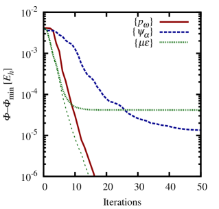
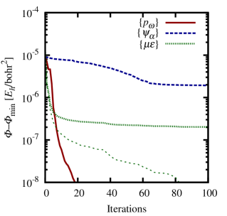
(a) 4 Å  hard sphere	(b) Capacitor with $E_{0}=1$ V/Å

Figure 1: Convergence of conjugate gradients minimization of the free energy of scalar-EOS water (a) surrounding a 4 Å  hard sphere, and (b) in a parallel plate capacitor with externally applied field strength $E_{0}=1$ V/Å, for different independent variables. The difference of free energy from the final equilibrium value as a function of iteration count is shown on a logarithmic scale for the self representation $\{p_{\omega}\}$ (solid red line), the site-potential representation $\{\psi_{\alpha}\}$ (blue dashed line), and the multipole representation $\{\mu,\vec{\epsilon}\}$ (thicker green dotted line). The fainter green dotted line is the difference of the free energy in the $\{\mu,\vec{\epsilon}\}$ representation from the converged value within that representation (which is variationally higher than the equilibrium value). Note the rapid exponential convergence in the self and multipole representations, compared to the site potential representation.

The hard sphere system consists of an external potential $V_{O}(\vec{r})=V_{0}\theta(R-|\vec{r}|)$ which excludes the $O$ sites of water from a sphere of radius $R$, with no potential on the $H$ sites ($V_{H}(\vec{r})=0$). We pick $R=4$ Å, a reasonable size for the region excluded by a molecule solvated in water, and $V_{0}=1~{}E_{h}$ ($\approx$ 27.2 eV) which is sufficient to completely exclude the liquid from that region. The calculations are performed in a cubic unit cell of side 32 bohrs ($\approx$ 17 Å) with a $128\times 128\times 128$ fast Fourier transform (FFT) grid; the grid spacing of 0.25 bohrs corresponds roughly to the charge density grid of a typical electronic density-functional theory calculation at a wave-function kinetic energy cutoff of 20 $E_{h}$.

The parallel plate capacitor system consists of two plates 112 bohrs apart, with an external potential corresponding to an applied electric field of $E_{0}=1$ V/Å ($10^{10}$ V/m), which is typical in the first solvation shell of a polar molecule, and corresponds to a regime of strongly non-linear dielectric response. (See Figure 8.) Repulsive potentials of strength 1 Eh on both the $O$ and $H$ sites confine the fluid to the region between the capacitor plates. The calculation is performed in a periodic cell of length 256 bohrs containing two capacitors back-to-back so that the cell has no net dipole, and is sampled using a one-dimensional FFT grid with 4096 points. The transverse dimensions are translationally invariant, and the free energies reported are per bohr² transverse area.

Figure 1 shows the convergence of the Polak-Ribiere variant of the nonlinear conjugate gradients algorithm [33] for the hard-sphere and capacitor systems with the site-potential ($\{\psi_{\alpha}\}$), $j=1$ truncated multipole ($\{\mu,\vec{\epsilon}\}$) and self ($\{p_{\omega}\}$) representations of the orientation density as independent variables. The initial guess in each case corresponds to a uniform bulk density of water in the allowed regions and no density in the disallowed regions, with a uniform orientation distribution for the sphere geometry, and a dipolar orientation distribution corresponding to bulk linear dielectric response for the capacitor geometry. The 7-design quadrature with 96 nodes on $SO(3)/\mathbb{Z}_{2}$ (see Table 1) was used for orientation sampling.

The self representation ($\{p_{\omega}\}$) exhibits the best exponential convergence, and is the method of choice when it is practical to store the orientation density. The multipole representation ($\{\mu,\vec{\epsilon}\}$) also converges quite rapidly, but it is a variational approximation and will result in a higher free energy than that in $\{p_{\omega}\}$. Note that for a typical molecule cavity formation (the hard sphere case), the error in the $\{\mu,\vec{\epsilon}\}$-representation is $\sim 4\times 10^{-5}~{}E_{h}$ or $\sim 0.03$ kcal/mol, which is negligible in the computation of solvation energies. Likewise, the relative error in the free energy of the strong-field capacitor corresponds to an error of less than $\sim 1\%$ in the effective dielectric constant, which again is acceptable in the calculation of solvation energies. Finally, the site-potential representation ($\{\psi_{\alpha}\}$) of [10, 12] exhibits the poorest convergence, particularly in the strong electric field case. Although the $\{\psi_{\alpha}\}$ entropy will eventually converge to the same value as that of the $\{p_{\omega}\}$ representation, the approximate $\{\mu,\vec{\epsilon}\}$ representation yields a more accurate free energy at practical iteration counts.

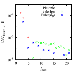
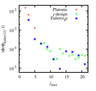
(a) 4 Å  hard sphere	(b) Capacitor with $E_{0}=1$ V/Å

Figure 2: Convergence of free energy with orientation quadrature for the two systems considered in Figure 1. The orientation quadratures studied are listed in Table 1, and the free energy at the Euler(12) quadrature (which has 3456 nodes on $SO(3)/\mathbb{Z}_{2}$) is used as the reference in computing relative errors for all the smaller quadratures. Note that the error due to the orientation quadrature plateaus at $j_{max}\sim 7$ for the sphere geometry, and at $j_{max}\sim 10$ for the strong-field capacitor; these would therefore be reasonable choices in ab initio solvation calculations for non-polar and strongly-polar molecules respectively.

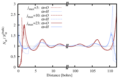
(a) 4 Å  hard sphere	(b) Capacitor with $E_{0}=1$ V/Å

Figure 3: Convergence of density profiles with orientation quadrature for the two systems considered in Figure 1. The plotted site-densities are scaled by their corresponding bulk values, so that the profiles equilibrate at 1 far from the sphere / plates. Note that the densities at the lowest and highest quadratures are indistinguishable for the hard sphere, whereas the densities become similar to the fully-converged ones only around $j_{max}\sim 10$ for the strong-field capacitor.

Next, we turn to the convergence of the free energies with respect to the discretization of the orientation integrals. Figure 2 shows the relative error in the free energy for each orientation quadrature in Table 1 compared to the Euler(12) quadrature (taken to be the converged value) for the two systems considered above. The quadratures are sorted by $j_{max}$, the maximum degree of Wigner functions $D^{j}_{m_{1}m_{2}}$ for which they are exact. (See A for details.) The relative error in the free energy decreases rapidly with quadrature size and plateaus $\sim 10^{-7}$ at $j_{max}\sim 7$ for the hard sphere, limited by other discretization errors. For the highly polarized capacitor, higher quadratures are needed for the same level of accuracy, and the plateau occurs $\sim 10^{-4}$ at $j_{max}\sim 10$. A reasonable choice for $j_{max}$ for a typical system should therefore range from 7 to 10 depending on the strength of electric fields involved.

Figure 3 shows the density profiles next to the hard sphere and the walls of the capacitor for various orientation quadratures. In the case of the hard sphere, the density profiles are virtually identical for all considered quadratures, as is expected given that the relative error in the free energy is $\sim 10^{-4}$ even for the Octahedron group, one of the lowest quadratures considered with $j_{max}=3$. However, there are qualitative differences in the density profiles near the capacitor walls for $j_{max}=3$ from the converged ones at $j_{max}=23$ (Euler(12) quadrature), and the differences begin to disappear only around $j_{max}=10$. At these field strengths, the orientation distribution is highly polarized (close to saturation) and hence requires a dense orientation quadrature to resolve. (The orientation distribution approaches a $\delta$-function in the limit of infinite electric field.)

4.3 Accuracy of water functionals

Finally, we turn to a comparison of the excess functionals for water suitable for ab initio solvation methods. In particular, we focus on the scalar-EOS functional of section 3.2, the bonded-voids functional [27] and the functional of Lischner et al. [13]. The last functional is based on experimental correlations functions, which we will refer to as the ‘fitted-correlations’ functional. We perform all calculations in one-dimensional planar or radial grids, using the Fluid1D sub-project of JDFTx [30]. We use the Euler(20) orientation quadrature, with $n_{\alpha}=1$ to exploit rotational symmetry in the transverse directions. (See B.)

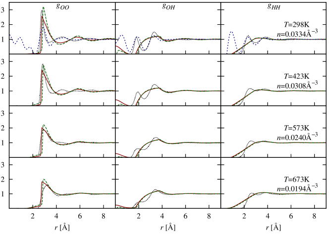
Figure 4: Partial radial distributions (site-site correlation functions) for the scalar-EOS water functional (solid red lines), bonded-voids functional [27] (long-dashed green lines) and fitted-correlations functional [13] (short-dashed blue lines), compared to experimental pair correlations of water from Soper et al. [34] (black dotted lines). The position and location of the first $g_{OO}$ peak for scalar-EOS and bonded-voids are in reasonable agreement with experiment, but the remaining structure resembles that of a close-packed hard sphere fluid rather than a tetrahedrally bonded one. The fitted-correlations functional is defined only at 298 K and captures the features of the correlation functions by construction, but suffers from short-ranged artifacts due to the bandwidth-limited fitting procedure of [13].

First we examine the pair correlation functions $g_{\alpha\beta}$ of the bulk fluid computed using the Ornstein-Zernike relation for the rigid-molecular fluid which may be written as

$$\tilde{h}=(1-\tilde{I}\tilde{c}\bar{N})^{-1}\tilde{I}\tilde{c}\tilde{I},$$ (37)

which is a matrix equation in Fourier space for each wave vector $k$. Here, $\tilde{h}_{\alpha\beta}(k)$ is the Fourier transform of $g_{\alpha\beta}(r)-1$, $\tilde{I}_{\alpha\beta}(k)=j_{0}(kR_{\alpha\beta})$ is the intra-molecular structure factor with $R_{\alpha\beta}$ being the distance between sites $\alpha$ and $\beta$ within the molecule, $\bar{N}$ is the bulk number density of fluid molecules, and $\tilde{c}_{\alpha\beta}(k)$ is the Fourier transform of the direct correlation function $c_{\alpha\beta}(\vec{r}-\vec{r}^{\prime})=(-1/T)\delta^{2}F_{\textrm{ex}}/\delta N_{\alpha}(\vec{r})\delta N_{\beta}(\vec{r}^{\prime})$ evaluated in the limit of the uniform fluid.

The direct correlation functions are computed analytically in Fourier space for a set of wave vectors corresponding to the spherical Bessel function basis with 1024 basis functions and a radial extent $r_{\textrm{max}}=64$ bohrs (see B), and the pair correlation functions are computed via (37) using numerical spherical Bessel transforms. Figure 4 compares the pair correlations for all three functionals under consideration compared against those obtained by Soper et al [34] from neutron diffraction data by empirical-potential structure refinement (EPSR).

The scalar-EOS functional correctly captures the location and height of the first peak in $g_{OO}(r)$, but produces a secondary structure reminiscent of the close-packed coordination of the hard sphere fluid rather than the tetrahedral coordination exhibited by water. The split hydrogen peaks in the experimental data are fused into a single broader one with the same particle content. These are qualitatively the same features as the bonded-voids functional, but with slightly better agreement for the scalar-EOS functional. After all, the motivation for the scalar-EOS functional was to simplify the bonded-voids functional because it captured free energies of cavity formation reasonably despite not exhibiting features of tetrahedral correlation. The fitted-correlations functional reproduces some of the features of the experimental correlation functions by construction, but exhibits artifacts at short distances due to the bandwidth limitation in the fitting procedure for the correlations (and partly because it does not employ a hard sphere reference).

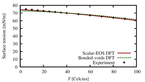
Figure 5: Energy of the planar vapor-liquid interface for the scalar-EOS and bonded-voids water functionals as a function of temperature, compared to the experimental values for surface tension [35]. Both functionals fit the range parameter of the Lennard-Jones pair potential to the experimental surface tension at 298 K, and the scalar-EOS functional reproduces the temperature dependence more accurately than the bonded-voids one. (The fitted-correlations functional is omitted from this plot, since it is defined only at 298 K.)

Next, we examine the free energies of planar liquid-vapor interface for each functional. The calculations are performed on a one-dimensional planar grid of length 96 bohrs with 768 sample points and basis functions. For each temperature, the pressure is adjusted to the boiling point, which corresponds to equal chemical potentials and bulk grand free energy densities for the two phases. The hard sphere radius $R_{\textrm{HS}}=1.36$ Å  for the scalar-EOS functional was determined by matching the interface energy obtained from such a calculation at 298 K to the experimental value for the surface tension 72.0 mN/m. Figure 5 compares the temperature dependence of this interface energy against experimental values for the surface tension. The scalar-EOS functional captures the trend in the experimental data slightly better than the bonded-voids functional.

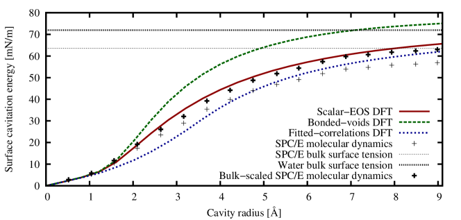
Figure 6: Variation of the solvation energy of hard spheres that exclude the oxygen sites of water from their interior, with the radius of such spheres, compared to the SPC/E molecular dynamics results of [36]. The SPC/E model underestimates the bulk surface tension of water by $10\%$ [37], and we have included a scaled version of the SPC/E data as a reasonable guess for real water. The scalar-EOS functional agrees with the bulk-scaled SPC/E data accurately, while the fitted-correlations functional systematically underestimates and the bonded-voids functional overestimates the free-energy of cavity formation.

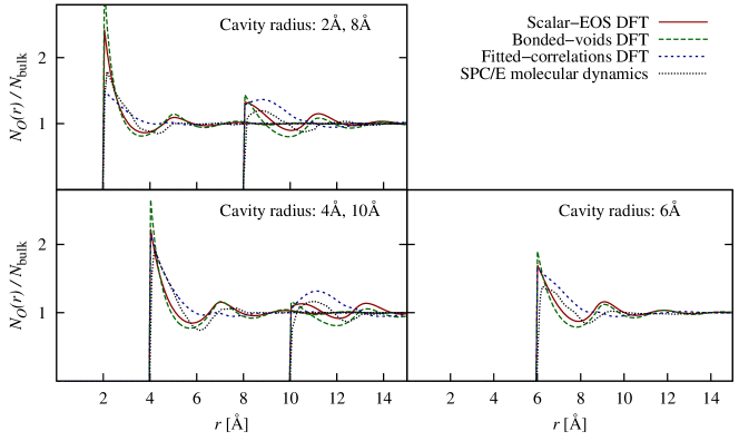
Figure 7: Radial density profiles around hard spheres that exclude the oxygen sites of water from their interior, for spheres of radius 2, 4, 6, 8 and 10 Å, compared to the SPC/E molecular dynamics results of [36]. The fitted-correlations functional misses the secondary peaks in the profiles, while the scalar-EOS and bonded-voids functional overestimate the contact density and the secondary structure, with best agreement provided by the scalar-EOS model.

The planar interface energies provide a means to calibrate the liquid functionals against experimental measurements, and the excellent agreement for the temperature dependence after adjusting the surface tension at one temperature is promising. However, the applicability of a functional for molecular solvation calculations depends on its ability to accurately describe the free energies required to form cavities of molecular dimensions. A standard test case is the solvation free energy for microscopic hard spheres in the fluid. We compute the cavitation energies for hard spheres of radii $R$ ranging from 0 to 9 Å, with external potentials $V_{O}(r)=(1~{}E_{h})\theta(R-r)$ and $V_{H}(r)=0$ that exclude the oxygen site of water from the interior of the spheres. The calculations are performed on a one-dimensional radial grid of extent $r_{\textrm{max}}=64$ bohrs ($\approx 34$ Å) with 512 sample points and basis functions.

Figure 6 compares the variation of the hard sphere solvation energy per surface area with sphere radius for all three functionals with SPC/E molecular dynamics estimates for the same from [36]. For large spheres, the surface curvature effects become negligible and the surface energy approaches the planar surface tension; whereas for small enough spheres the cavitation energy is proportional to the volume ($\Delta\Phi=N_{\textrm{bulk}}T\times(4\pi R^{3}/3)$, so that $\Delta\Phi/(4\pi R^{2})\propto R$). Note that all three functionals agree perfectly with the molecular dynamics results in the small radius limit, and they all approach the bulk experimental surface tension in the large radius limit (after overshooting the bulk value in the bonded-voids case). However the SPC/E model underestimates the bulk surface tension to be 65 mN/m [37] compared to the experimental value of 72 mN/m, and therefore the molecular dynamics results for the sphere solvation energies are also underestimated by a similar amount for the larger spheres. Consequently, we include the molecular dynamics results scaled up by the ratio of experimental to SPC/E surface tensions as a reasonable guess for the hard sphere cavitation energy of real water in Figure 6 (in addition to the unscaled values). The scalar-EOS functional significantly outperforms bonded-voids and fitted-correlations in its agreement with the bulk-scaled molecular dynamics results, and is the best candidate for an accurate density functional description of cavitation energies in liquid water.

We next examine the distribution of water around these spherical cavities of selected sizes in Figure 7. As expected from the results for the free energies, the density profiles of the scalar-EOS functional are in closest agreement with the SPC/E molecular dynamics results of [36]. The bonded-voids functional overestimates the structure in the liquid, which is expected since it also overestimated the structure in the pair correlations (Figure 4). The fitted-correlations functional severely underestimates the secondary structure in the density profiles despite better qualitative agreement with the experimental pair correlation functions.

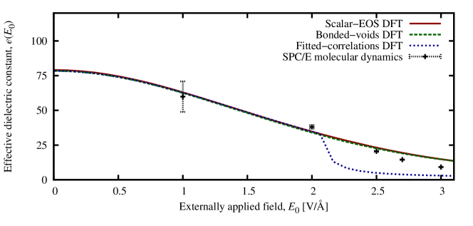
Figure 8: Nonlinear dielectric response of the water functionals compared to SPC/E molecular dynamics results from [38]. All three functionals provide essentially the same dielectric response, as this is determined by a competition between the molecular ideal gas entropy and the scaled mean field electrostatics. The minor differences arise from differences in the equations of state due to electrostriction (change of bulk-density in strong fields). The fitted-correlations functional has an unphysical instability accompanied by a rapid increase in density and drop in dielectric constant at an external field $\approx 2$ V/Å, due to an underestimation of the compressibility at high pressures by its polynomial excess free energy density model.

Finally, we turn to the last key ingredient for a successful theory of solvation: nonlinear dielectric response. The typical electric fields in the vicinity of polar molecules are $\sim$ V/Å  i.e. $10^{10}$ V/m, which corresponds to strong non-linearities and significant dielectric saturation. Here, we examine the nonlinear dielectric constant defined by $\epsilon(E_{0})=E_{0}/(E_{0}-4\pi P)$, where $E_{0}$ is a macroscopic externally applied field and $P$ is the corresponding bulk polarization density in the liquid.

At equilibrium, a liquid in a macroscopic parallel-plate capacitor adopts uniform density and polarization except for microscopic regions around the plates. The free energy of that capacitor is dominated by the bulk; the regions next to the plates only contribute via long-range interactions of the bound sheet-charge densities $\pm P$ in the liquid. Accounting for the interaction of these sheet charges with the external field, and with each other via the scaled mean-field Coulomb interaction, we can show that the effective free energy density minimized by the macroscopic capacitor at equilibrium is

$$\phi(p_{\omega})=T\int\frac{\textrm{d}\omega}{8\pi^{2}}p_{\omega}\left(\log\frac{p_{\omega}}{N_{\textrm{ref}}}-1\right)-\sum_{\alpha}\mu_{\alpha}N_{\alpha}+f_{\textrm{ex}}(\{N_{\alpha}\})\\ -\vec{E}_{0}\cdot\vec{P}+A_{\epsilon}(T)\frac{4\pi P^{2}}{2}.$$

Here, $f_{\textrm{ex}}$ is the excess-free energy density of the uniform fluid (which is determined entirely by the equation of state) and $\vec{P}=\int\frac{\textrm{d}\omega}{8\pi^{2}}p_{\omega}\omega\circ\vec{P}_{\textrm{mol}}$ is the polarization density, with $\vec{P}_{\textrm{mol}}$ being the dipole moment of the fluid molecule in its reference orientation. We therefore minimize this free energy density on a planar grid with a single grid point to obtain the equilibrium $P$ for each applied $E_{0}$, thereby avoiding the need for setting up a capacitor in a large simulation cell.

All three functionals considered here employ the same scaled mean-field electrostatic interaction constrained to produce the bulk dielectric response as proposed by Lischner et al. [13]. The physics of dielectric saturation is captured by an interplay of this term with the entropy of the ideal gas of rigid molecules, which again is common to all three functionals. Consequently, their nonlinear dielectric response is very similar and compares quite well with the SPC/E molecular dynamics results [38] as shown in Figure 8. The minor differences between the functionals are due to the different uniform fluid excess free energy densities ($f_{\textrm{ex}}$) which correspond to different approximations to the equation of state of the fluid. The fitted-correlations functional employs a polynomial model for $f_{\textrm{ex}}$ obtained from the bulk modulus and its pressure derivative at ambient conditions [13], which underestimates the bulk modulus at high compression. This causes the instability at high fields associated with a rapid increase in density, seen as a drop in the dielectric response at $\approx 2$ V/Å  in Figure 8.

5 Conclusions

We construct a general framework for the classical density-functional theory of rigid-molecular fluids that avoids the inversion problem associated with site-density constraints by switching to the orientation density as the key variable. We show that the independent variables in previous solutions, such as ideal-gas effective site potentials, are compressed maximum-entropy representations of the orientation density. We then motivate other representations with superior convergence properties which are variational approximations to the free energy. The self-representation, directly minimizing over the orientation density $\{p_{\omega}\}$, exhibits the fastest convergence for conjugate gradients minimization, but requires memory in proportion to the size of the quadrature for orientation integrals. The site-potential representation $\{\psi_{\alpha}\}$, although exact in principle, is impractical due to poor convergence, particularly in the presence of strong electric fields. We introduce the multipole representation $\{\mu\vec{\epsilon}\}$ which exhibits comparable convergence to the self-representation without the memory overhead, is effectively more accurate than $\{\psi_{\alpha}\}$ at practical iteration counts despite being a (variational) approximation, and enables efficient large-scale ab initio solvation in polar molecular fluids within the framework of joint density-functional theory.

We extend the algebraic formulation of electronic density-functional theory, DFT++ [15], and present the discretization of our general framework and excess functionals for practical calculations in a basis-independent manner. The methods developed in this paper form the basis for the fluid sector of the open-source electronic density-functional theory software JDFTx [14], which provides a three-dimensional plane-wave basis implementation of this work. Additionally, a one dimensional version implementing the three basis sets of B is distributed as a sub-project of JDFTx [30], suitable for rapid prototyping and development of fluid functionals within this framework.

In addition to the general framework for polar fluids, we construct a practical free energy functional for liquid water which improves on the accuracy of earlier functionals, the bonded-voids model [27] based on Wertheim perturbation and the fitted-correlations model [13] based on experimental correlation functions of water, while minimizing complexity and avoiding over-parametrization. We show that this ‘scalar-EOS’ functional accurately captures the key quantities of interest for ab initio solvation calculations: free energies for formation of microscopic cavities in the fluid, and non-linear dielectric response. Within joint density-functional theory, the methods developed here provide an accurate and efficient description of solvent environments, thereby enabling a focused electronic structure study of solvated biological and chemical systems of technological relevance.

This work was supported as a part of the Energy Materials Center at Cornell (EMC²), an Energy Frontier Research Center funded by the U.S. Department of Energy, Office of Science, Office of Basic Energy Sciences under Award Number DE-SC0001086.

Appendix A Efficient quadratures for orientation integrals

Efficient discretization of the orientation integrals is critical to the performance of any of the representations of Section 2.2 and determines the very practicality of the $p_{\omega}$ (self) representation. Here, we list efficient quadratures for discretizing integrals over $\omega$, $\int\frac{\textrm{d}\omega}{8\pi^{2}}f(\omega)\to\sum_{i}W_{i}f(\omega_{i})$.

The simplest approach is to label orientations by ZYZ-Euler angles $\omega=(\alpha,\beta,\gamma)$ and use the outer product of a Gauss-Legendre quadrature for $\beta\in[0,\pi]$ and Gauss-Fourier quadratures for the periodic $\alpha,\gamma\in[0,2\pi)$. More efficient quadratures may be constructed as an outer product using the $\mathbb{S}_{2}\times\mathbb{S}_{1}$ structure of $SO(3)$, or by working directly on $SO(3)$ without an outer product structure [39].

In [39], quadratures on $SO(3)$ are optimized to minimize the RMS error in the integrals of all $D^{j}_{m_{1}m_{2}}(\omega)$ up to some $j_{\textrm{max}}$. We focus on quadratures that are exact up to some $j_{\textrm{max}}$,

$$\sum_{i}W_{i}D^{j}_{m_{1}m_{2}}(\omega_{i})=\sum_{i}W_{i}d^{j}_{m_{1}m_{2}}(\beta_{i})\textrm{e}^{i(m_{1}\alpha_{i}+m_{2}\gamma_{i})}~{}=~{}\delta_{j0}$$ (38)

for all $|m_{1}|,|m_{2}|\leq j\leq j_{\textrm{max}}$, and can be optimized further using the symmetry of the molecule at hand. For simplicity, we only consider $\mathbb{Z}_{n}$ symmetry about a single axis, chosen to be the $z$-axis of the molecule frame without loss of generality. The quadratures considered then fall into 3 classes:

1. Symmetry groups of Platonic solids [39]

2. Outer products of a spherical $j$-design [40] on $\mathbb{S}_{2}(\alpha,\beta)$ with a uniform quadrature on $\mathbb{S}_{1}(\gamma)$

3. Outer product quadrature on all 3 Euler angles $\alpha$, $\beta$ and $\gamma$.

Each of these these classes consists of uniformly spaced nodes of equal weights in $\gamma$ for each $(\alpha,\beta)$. Grouping the nodes as $(\alpha_{k},\beta_{k},\gamma_{k}+2n\pi/n_{\gamma})$ for $n\in 0,\ldots,n_{\gamma}-1$ with total weight $W_{k}$ for each group, (38) can be reduced to

$$\sum_{k}W_{k}d^{j}_{m_{1}m_{2}}(\beta_{k})\textrm{e}^{i(m_{1}\alpha_{k}+m_{2}\gamma_{k})}=\delta_{j0}$$ (39)

for all $|m_{1}|,|m_{2}|\leq j\leq j_{\textrm{max}}$ such that $m_{2}$ is a multiple of $n_{\gamma}$. Therefore if $n_{\gamma}>j_{\textrm{max}}$ (which is the case for all but the Icosahedron rotation group), (39) further simplifies to

$$\sqrt{4\pi}\sum_{k}W_{k}Y^{j}_{m}(\beta_{k},\alpha_{k})=\delta_{j0}$$ (40)

for all $|m|\leq j\leq j_{\textrm{max}}$ using the relations of $D^{j}_{m0}$ to the spherical harmonics.

A spherical $j_{\textrm{max}}$-design is a set of points on the unit sphere that satisfies (40) with uniform weights $W_{k}$, and hence it yields an $SO(3)$ quadrature exact to $j_{\textrm{max}}$ when combined with a uniform quadrature with $j_{\textrm{max}}+1$ nodes on $\mathbb{S}_{1}(\gamma)$. We use the spherical designs with the smallest number of nodes for each $7\leq j_{\textrm{max}}\leq 21$ tabulated in [40] to form the quadratures of class (b). The quadratures of lower order reduce to class (a), specifically the rotation groups of the Tetrahedron at $j_{\textrm{max}}=2$, Octahedron at $j_{\textrm{max}}=3$ and Icosahedron at $j_{\textrm{max}}=5$.

The Gauss-Legendre quadrature with $n_{\beta}$ nodes on $\cos\beta\in[-1,1]$ is exact for the integration of all polynomials up to order $2n_{\beta}-1$. The outer product of this with a uniform quadrature with $2n_{\beta}$ nodes on $\alpha\in[0,2\pi)$ satisfies (40) for $j_{\textrm{max}}=2n_{\beta}-1$, and hence also (38) to that order when combined with $2n_{\beta}$ uniform samples on $\gamma$.

Finally the reduction by $\mathbb{Z}_{n}$ symmetry about the $z$-axis in the molecule frame amounts to replacing $\mathbb{S}_{1}(\gamma)$ with $\mathbb{S}_{1}/\mathbb{Z}_{n}$. This is achieved by a uniform sampling of $\lceil n_{\gamma}/n\rceil$ points on $\gamma\in[0,2\pi/n)$, which retains the exactness to $j_{\textrm{max}}$ for functions with this symmetry with a reduction of up to $n$ in the number of nodes required.

The accuracy of these quadratures for the classical density functional theory of rigid molecules is explored in section 4.2. The quadratures considered there are listed in Table 1 along with their $j_{\textrm{max}}$, the number of nodes for sampling $SO(3)/\mathbb{Z}_{n}$ in general and $SO(3)/\mathbb{Z}_{2}$ in particular, which is the case relevant for water. Note that the Euler quadrature with $n_{\beta}=3$ needs almost twice as many nodes as the Icosahedron group for the same $j_{\textrm{max}}=5$, but the relative inefficiency of the Euler quadratures decreases with $j_{\textrm{max}}$ and becomes less than $1\%$ between the $n_{\beta}=11$ Euler quadrature and the 21-design at $j_{\textrm{max}}=21$.

	$j_{\textrm{max}}$	Number of quadrature nodes for
		$SO(3)/\mathbb{Z}_{n}$	$SO(3)/\mathbb{Z}_{2}$
Tetrahedron	2	$4\times\lceil 3/n\rceil$	8
Octahedron	3	$6\times\lceil 4/n\rceil$	12
Icosahedron	5	$12\times\lceil 5/n\rceil$	36
7-design	7	$24\times\lceil 8/n\rceil$	96
8-design	8	$36\times\lceil 9/n\rceil$	180
9-design	9	$48\times\lceil 10/n\rceil$	240
10-design	10	$60\times\lceil 11/n\rceil$	360
11-design	11	$70\times\lceil 12/n\rceil$	420
12-design	12	$84\times\lceil 13/n\rceil$	588
13-design	13	$94\times\lceil 14/n\rceil$	658
14-design	14	$108\times\lceil 15/n\rceil$	864
15-design	15	$120\times\lceil 16/n\rceil$	960
16-design	16	$144\times\lceil 17/n\rceil$	1296
17-design	17	$156\times\lceil 18/n\rceil$	1404
18-design	18	$180\times\lceil 19/n\rceil$	1800
19-design	19	$204\times\lceil 20/n\rceil$	2040
20-design	20	$216\times\lceil 21/n\rceil$	2376
21-design	21	$240\times\lceil 22/n\rceil$	2640
Euler$(n_{\beta})$	$2n_{\beta}-1$	$2n_{\beta}^{2}\times\lceil 2n_{\beta}/n\rceil$	$2n_{\beta}^{3}$

Table 1: List of explored quadratures, their degree of exactness $j_{\textrm{max}}$, and the number of nodes in sampling $SO(3)/\mathbb{Z}_{n}$. The Euler angles corresponding to the platonic solid rotation groups are listed in [39]. The $j$-designs are constructed as an outer product of the spherical $j$-designs with fewest points for each $j$ from [40] used for $(\alpha,\beta)$ with $\lceil(j+1)/n\rceil$ uniform samples on $\gamma\in[0,2\pi/n)$. Each Euler$(n_{\beta})$ quadrature is an outer product of a $n_{\beta}$-point Gauss-Legendre quadrature on $\cos\beta\in[-1,1]$, a uniform $2n_{\beta}$-point quadrature on $\alpha\in[0,2\pi)$, and a uniform $\lceil 2n_{\beta}/n\rceil$-point quadrature on $\gamma\in[0,2\pi/n)$.

Appendix B One-dimensional discretization for special geometries

The discretization of three-dimensional space according to Section 4.1, along with the orientation quadratures of A provide a practical route to computations with the rigid-molecular classical density functional framework of Section 2 in arbitrary geometries and basis sets. However, the development and testing of new excess functionals for liquids primarily require calculations in high-symmetry configurations. Here, we detail the formulation of highly-efficient discretizations of planar, cylindrical and spherical geometries on a one-dimensional grid, which allow for the rapid prototyping of excess functionals employed in Section 4.3 and [27].

The discretization of space is performed in the framework of Section 4.1, but with special basis sets exploiting the symmetry. The three geometries we consider here are

1. Planar, where all spatial dependence is along $z$,

2. Cylindrical, with dependence only on the distance from the $z$-axis $\rho$, and

3. Spherical, with dependence only on distance from origin $r$.

Each of these geometries require only a one-dimensional discretization. For the planar geometry, we impose mirror-symmetry boundary conditions at the ends of the grid, and pick a basis of cosines and a corresponding quadrature grid suited for the Discrete Cosine Transform [41]. For the spherical and cylindrical geometries, we impose Neumann boundary conditions at some maximum radius, and choose a finite basis of spherical and cylindrical Bessel functions respectively, along with a quadrature grid suited for the Discrete Bessel Transform [42] . The definition of the basis functions, quadrature grid and the matrix elements for the operators of Section 4.1 are summarized in Table 2.

	Planar	Cylindrical	Spherical
CoordinateSystem	$(x,y,z)$	$(\rho,\phi,z)$	$(r,\theta,\phi)$
Symmetry	$f(\vec{r})\to f(z)$	$f(\vec{r})\to f(\rho)$	$f(\vec{r})\to f(r)$
Boundaryconditions	$f^{\prime}(0)=f^{\prime}(L)=0$	$f^{\prime}(\rho_{\textrm{max}})=0$	$f^{\prime}(r_{\textrm{max}})=0$
Basis $b_{i}(\vec{r})$	$\begin{array}[]{l}\tilde{w}_{i}\cos(G_{i}z),\\ G_{i}=i\pi/L,\\ \tilde{w}_{i}=\frac{2}{(1+\delta_{i0})L}\end{array}$	$\begin{array}[]{l}\tilde{w}_{i}J_{0}(G_{i}\rho),\\ G_{i}=Y_{i}/\rho_{\textrm{max}},\\ \tilde{w}_{i}=\frac{J_{0}^{-2}(Y_{i})}{\pi\rho_{\textrm{max}}^{2}}\end{array}$	$\begin{array}[]{l}\tilde{w}_{i}j_{0}(G_{i}r),\\ G_{i}=y_{i}/r_{\textrm{max}},\\ \tilde{w}_{i}=\frac{j_{0}^{-2}(y_{i})}{\left(2-\frac{2}{3}\delta_{i0}\right)\pi r_{\textrm{max}}^{3}}\end{array}$
Quadraturegrid $\{\vec{r}_{j}\}$	$z_{j}=(j+\frac{1}{2})\frac{L}{S}$	$\rho_{j}=X_{j+1}\frac{\rho_{\textrm{max}}}{Y_{S}}$	$r_{j}=x_{j+1}\frac{r_{\textrm{max}}}{y_{S}}$
$\mathcal{I}_{ji}$	$\tilde{w}_{i}\cos\left((j+\frac{1}{2})\pi\frac{i}{S}\right)$	$\tilde{w}_{i}J_{0}\left(X_{j+1}\frac{Y_{i}}{Y_{S}}\right)$	$\tilde{w}_{i}j_{0}\left(x_{j+1}\frac{y_{i}}{y_{S}}\right)$
$\mathcal{J}_{ij}$	$\begin{array}[]{l}w_{j}\cos\left((j+\frac{1}{2})\pi\frac{i}{S}\right),\\ w_{j}=\frac{L}{S}\end{array}$	$\begin{array}[]{l}w_{j}J_{0}\left(X_{j+1}\frac{Y_{i}}{Y_{S}}\right),\\ w_{j}=\frac{4\pi\rho_{\textrm{max}}^{2}}{Y_{S}^{2}J_{1}^{2}(X_{j+1})}\end{array}$	$\begin{array}[]{l}w_{j}j_{0}\left(x_{j+1}\frac{y_{i}}{y_{S}}\right),\\ w_{j}=\frac{4\pi^{2}r_{\textrm{max}}^{3}}{y_{S}^{3}j_{1}^{2}(x_{j+1})}\end{array}$
$\mathcal{O}_{i^{\prime}i}$	$\tilde{w}_{i}\delta_{i^{\prime}i}$
$\mathcal{L}_{i^{\prime}i}$	$-G_{i}^{2}\tilde{w}_{i}\delta_{i^{\prime}i}$
$(\mathcal{J^{\dagger}OJ})_{j^{\prime}j}$	$w_{j}\delta_{j^{\prime}j}$
$(g(r)\ast)_{i^{\prime}i}$	$\delta_{i^{\prime}i}\int 4\pi r^{2}\textrm{d}rg(r)j_{0}(G_{i}r)$

Table 2: Definition of the basis functions for the high-symmetry geometries - planar, cylindrical and spherical - with one-dimensional discretizations of sample count $S$, and matrix elements of the operators of Section 4.1 for each of these basis sets. The basis functions are labeled by $i=0,1,\cdots,S-1$ for each basis set, and $X_{i}$, $x_{i}$, $Y_{i}$ and $y_{i}$, are the $i^{\textrm{th}}$ roots of $J_{0}(x)$, $j_{0}(x)$, $J_{0}^{\prime}(x)$ and $j_{0}^{\prime}(x)$ respectively, with $Y_{0}=y_{0}\equiv 0$. The quadrature grid has the same number of points $S$ as the basis size, and are labeled by $j=0,1,\cdots,S-1$.

All three basis sets are derived from the eigenfunctions of the three-dimensional Laplace equation in various geometries, and are therefore intricately linked to the three-dimensional plane-wave basis: the basis functions are indexed by $G_{i}$, the magnitude of the corresponding plane-wave momentum. Consequently, the Laplacian and convolutions by spherical functions are diagonal in these basis sets as well, as indicated in Table 2. The transform operators $\mathcal{I}$ and $\mathcal{J}$ reduce to the ‘DCT type III’ and ‘DCT Type II’ fast Fourier transforms [43] respectively in the planar geometry (or ‘IDCT’ and ‘DCT’ in the notation of [41]); the cylindrical and spherical transforms lack an analogous $\mathcal{O}(S\log S)$ method and are implemented as matrix-vector multiplies with a precomputed Bessel function matrix.

The basis-independent discretization of the scalar-EOS excess functional (35), and site-density excess functionals in general, carries over to the planar, cylindrical and spherical geometries without modification. The discretization of the rigid-molecular ideal gas free energy and the generation of site-densities from independent variables carries over unmodified for the planar geometry, but is slightly complicated for the cylindrical and spherical geometries by the fact that the translation operator breaks the symmetry of the basis set and does not have a one-dimensional representation.

We can however compute the site-densities using (34) and the orientation-density in the site-potential representation using (31) for these basis sets as well, with minor modifications to the translation operators in those equations. First, we pick a covariant reference orientation for the molecule, (relative to the local coordinate frame $(\hat{\rho},\hat{\phi},\hat{z})$ or $(\hat{r},\hat{\theta},\hat{\phi})$), so that $p_{\omega}(\vec{r})$ is invariant under the cylindrical or spherical symmetry for each $\omega$ and permits a one-dimensional representation. Consequently, the translations involved in (34) and (31) would be relative to the local coordinate frame as well, and hence position-dependent; we therefore need to generalize the translation operators $\mathcal{T}_{\vec{a}}$ to ‘warp’ operators $\mathcal{T}_{\vec{a}(\vec{r})}$ defined by $\mathcal{T}_{\vec{a}(\vec{r})}f(\vec{r})=f(\vec{r}+\vec{a}(\vec{r}))$. It can be shown that the expressions of Section 4.1 remain valid without modification upon this generalization.

The translation operator for the planar basis is a simple one-dimensional restriction of its three-dimensional counterpart, and it generalizes to

$$\mathcal{T}_{\vec{a}(\rho)}f(\rho)=f\left(\sqrt{(\rho+\vec{a}\cdot\hat{\rho})^{2}+(\vec{a}\cdot\hat{\phi})^{2}}\right)$$ (41)

for the cylindrical basis with $f(\rho)\equiv f(2\rho_{\textrm{max}}-\rho)$ for $\rho>\rho_{\textrm{max}}$, and

$$\mathcal{T}_{\vec{a}(r)}f(r)=f\left(\sqrt{r^{2}+a^{2}+2r\vec{a}\cdot\hat{r}}\right)$$ (42)

for the spherical basis with $f(r)\equiv f(2r_{\textrm{max}}-r)$ for $r>r_{\textrm{max}}$. We could compute the matrix elements of these operators in the Bessel basis and apply the translation as a dense-matrix multiply in basis space, but those suffer from Nyquist frequency ringing problems similar to their three-dimensional counterparts. Instead, we compute these operators in real space using approximate sampling operators $\mathcal{S}_{\vec{a}(\vec{r})}$ based on constant or linear-spline interpolation which preserve non-negativity of scalar fields.

The results for the scalar-EOS water functional in Section 4.3 and the bonded-voids water functional in [27] were computed using the discretization scheme of Section 4.1, in the planar and spherical bases, with the warp operator $\mathcal{S}$ computed using linear-spline interpolation as discussed above. The planar and spherical bases have an additional rotational symmetry about the local $\hat{z}$ and $\hat{r}$ axes respectively at any point in space which renders the integral over Euler angle $\alpha$ trivial, so that a quadrature on $\mathbb{S}_{2}(\gamma,\beta)$ with no $\alpha$ sampling suffices; the one-dimensional calculations employ this additional optimization by using the Euler($n_{\beta}$) quadratures of A, but with $n_{\alpha}=1$ irrespective of $n_{\beta}$.

References

- Barker and Henderson [1976] J. A. Barker, D. Henderson, Rev. Mod. Phys. 48 (1976) 587.
- Ishizuka et al. [2008] R. Ishizuka, S.-H. Chong, F. Hirata, J. Chem. Phys. 128 (2008) 034504.
- Mermin [1965] N. D. Mermin, Phys. Rev. 137 (1965) A1441.
- Petrosyan et al. [2007] S. A. Petrosyan, J.-F. Briere, D. Roundy, T. A. Arias, Phys. Rev. B 75 (2007) 205105.
- Car and Parrinello [1985] R. Car, M. Parrinello, Phys. Rev. Lett. 55 (1985) 2471.
- Rosenfeld [1989] Y. Rosenfeld, Phys. Rev. Lett. 63 (1989) 980.
- Roth [2010] R. Roth, J. Phys. Cond. Matt. 22 (2010) 063102.
- Frodl and Dietrich [1992] P. Frodl, S. Dietrich, Phys. Rev. A 45 (1992) 7330.
- Chandler et al. [1986a] D. Chandler, J. McCoy, S. Singer, J. Chem. Phys. 85 (1986a) 5971.
- Chandler et al. [1986b] D. Chandler, J. McCoy, S. Singer, J. Chem. Phys. 85 (1986b) 5978.
- Ding et al. [1987] K. Ding, D. Chandler, S. J. Smithline, A. D. J. Haymet, Phys. Rev. Lett. 59 (1987) 1698.
- Lischner and Arias [2008] J. Lischner, T. A. Arias, Phys. Rev. Lett. 101 (2008) 216401.
- Lischner and Arias [2010] J. Lischner, T. A. Arias, J. Phys. Chem. B 114 (2010) 1946.
- Sundararaman et al. [2012a] R. Sundararaman, K. Letchworth-Weaver, T. A. Arias, JDFTx, http://jdftx.sourceforge.net, 2012a.
- Ismail-Beigi and Arias [2000] S. Ismail-Beigi, T. A. Arias, Comp. Phys. Comm. 128 (2000) 1.
- Wigner [1959] E. P. Wigner, Group theory and its application to the quantum mechanics of atomic spectra, Academic Press, New York, 1959.
- Percus [1976] J. K. Percus, Journal of Statistical Physics 15 (1976) 505.
- Wertheim [1963] M. S. Wertheim, Phys. Rev. Lett. 10 (1963) 321.
- Hansen-Goos and Roth [2006] H. Hansen-Goos, R. Roth, J. Phys.: Cond. Matt. 18 (2006) 8413.
- Carnahan and Starling [1969] N. F. Carnahan, K. E. Starling, J. Chem. Phys. 51 (1969) 635.
- Tarazona [2000] P. Tarazona, Phys. Rev. Lett. 84 (2000) 694.
- Weeks et al. [1971] J. D. Weeks, D. Chandler, H. C. Andersen, J. Chem. Phys. 54 (1971) 5237.
- Peng and Yu [2008] B. Peng, Y.-X. Yu, J. Phys. Chem. B 112 (2008) 15407.
- Curtin and Ashcroft [1985] W. A. Curtin, N. W. Ashcroft, Phys. Rev. A 32 (1985) 2909.
- Wertheim [1987] M. S. Wertheim, J. Chem. Phys. 87 (1987) 7323.
- Clark et al. [2006] G. N. I. Clark, A. J. Haslam, A. Galindo, G. Jackson, Molecular Physics 104 (2006) 3561.
- Sundararaman et al. [2012b] R. Sundararaman, K. Letchworth-Weaver, T. A. Arias, J . Chem. Phys. 137 (2012b) 044107.
- Berendsen et al. [1987] H. J. C. Berendsen, J. R. Grigera, T. P. Straatsma, J. Phys. Chem. 91 (1987) 6269.
- Jefferey and Austin [1999] C. A. Jefferey, P. H. Austin, J. Chem. Phys 110 (1999) 484.
- Sundararaman and Arias [2012] R. Sundararaman, T. A. Arias, Fluid1D: a sub-project of JDFTx, http://jdftx.svn.sourceforge.net/svnroot/jdftx/trunk/fluid1D, 2012.
- Arias [267] T. A. Arias, Rev. Mod. Phys. 71 (267) 1999.
- Fletcher and Reeves [1964] R. Fletcher, C. M. Reeves, Comp. J. 7 (1964) 149.
- Polak and Ribiere [1969] E. Polak, G. Ribiere, Rev. Fr. Inform. Rech. Oper. 16 (1969) 35.
- Soper [2000] A. K. Soper, Chem. Phys. 258 (2000) 121.
- Dean [1999] J. A. Dean, Lange’s Handbook of Chemistry, McGraw-Hill, 15 edn., 1999.
- Huang et al. [2001] D. M. Huang, P. L. Geissler, D. Chandler, J. Phys. Chem. B 105 (2001) 6704.
- Vega and de Miguel [2007] C. Vega, E. de Miguel, J. Chem. Phys. 126 (2007) 154707.
- Yeh and Berkowitz [1999] I.-C. Yeh, M. Berkowitz, J. Chem. Phys. 110 (1999) 7935.
- Graf and Potts [2009] M. Graf, D. Potts, Num. Func. Anal. and Optim. 30 (2009) 665.
- Hardin and Sloane [2002] R. H. Hardin, N. J. A. Sloane, Spherical designs, a library of putatively optimal spherical t-designs, URL http://www.research.att.com/~njas/sphdesigns, 2002.
- Ahmed et al. [1974] N. Ahmed, T. Natarajan, K. R. Rao, IEEE Trans. Comp. C-23 (1974) 90.
- Lemoine [1994] D. Lemoine, J. Chem. Phys 101 (1994) 3936.
- Frigo and Johnson [2005] M. Frigo, S. G. Johnson, Proc. IEEE 93 (2005) 216.