Exploiting Symmetry in Tensors for High Performance:
Multiplication with Symmetric Tensors

Martin D. Schatz222 Department of Computer Science, Institute for Computational Engineering and Sciences, The University of Texas at Austin, Austin, TX.
Emails: martin.schatz@utexas.edu, ltm@cs.utexas.edu, rvdg@cs.utexas.edu.
   Tze Meng Low222 Department of Computer Science, Institute for Computational Engineering and Sciences, The University of Texas at Austin, Austin, TX.
Emails: martin.schatz@utexas.edu, ltm@cs.utexas.edu, rvdg@cs.utexas.edu.
   Robert A. van de Geijn222 Department of Computer Science, Institute for Computational Engineering and Sciences, The University of Texas at Austin, Austin, TX.
Emails: martin.schatz@utexas.edu, ltm@cs.utexas.edu, rvdg@cs.utexas.edu.
   Tamara G. Kolda444Sandia National Laboratories, Livermore, CA. Email: tgkolda@sandia.gov.
(Draft
)
Abstract

Symmetric tensor operations arise in a wide variety of computations. However, the benefits of exploiting symmetry in order to reduce storage and computation is in conflict with a desire to simplify memory access patterns. In this paper, we propose a blocked data structure (Blocked Compact Symmetric Storage) wherein we consider the tensor by blocks and store only the unique blocks of a symmetric tensor. We propose an algorithm-by-blocks, already shown of benefit for matrix computations, that exploits this storage format by utilizing a series of temporary tensors to avoid redundant computation. Further, partial symmetry within temporaries is exploited to further avoid redundant storage and redundant computation. A detailed analysis shows that, relative to storing and computing with tensors without taking advantage of symmetry and partial symmetry, storage requirements are reduced by a factor of O(m!)𝑂𝑚\displaystyle O\left(m!\right) and computational requirements by a factor of O((m+1)!/2m)𝑂𝑚1superscript2𝑚\displaystyle O\left((m+1)!/2^{m}\right), where m𝑚\displaystyle m is the order of the tensor. However, as the analysis shows, care must be taken in choosing the correct block size to ensure these storage and computational benefits are achieved (particularly for low-order tensors). An implementation demonstrates that storage is greatly reduced and the complexity introduced by storing and computing with tensors by blocks is manageable. Preliminary results demonstrate that computational time is also reduced. The paper concludes with a discussion of how insights in this paper point to opportunities for generalizing recent advances in the domain of linear algebra libraries to the field of multi-linear computation.

1 Introduction

A tensor is a multi-dimensional or m𝑚\displaystyle m-way array. Tensor computations are increasingly prevalent in a wide variety of applications [22]. Alas, libraries for dense multi-linear algebra (tensor computations) are in their infancy. The aim of this paper is to explore how ideas from matrix computations can be extended to the domain of tensors. Specifically, this paper focuses on exploring how exploiting symmetry in matrix computations extends to computations with symmetric tensors, tensors whose entries are invariant under any permutation of indices, and exploring how block structures and algorithms extend to computations with symmetric tensors.

Libraries for dense linear algebra (matrix computations) have long been part of the standard arsenal for computational science, including the BLAS interface [23, 12, 11, 17, 16], LAPACK [3], and more recent libraries with similar functionality, like the BLAS-like Interface Software framework (BLIS) [37], and libflame [41, 36]. For distributed memory architectures, the ScaLAPACK [10], PLAPACK [35], and Elemental [27] libraries provide most of the functionality of the BLAS and LAPACK. High-performance implementations of these libraries are available under open source licenses.

For tensor computations, no high-performance general-purpose libraries exist. The MATLAB Tensor Toolbox [5, 4] defines many commonly used operations that would be needed by a library for multilinear algebra but does not have any high-performance kernels nor special computations or data structures for symmetric tensors. The PLS Toolbox [13] provides users with operations for analyzing data stored as tensors, but does not expose the underlying system for users to develop their own set of operations. Targetting distributed-memory environments, the Tensor Contraction Engine (TCE) project [7] focuses on sequences of tensor contractions and uses compiler techniques to reduce workspace and operation counts. The Cyclops Tensor Framework (CTF) [33] focuses on exploiting symmetry in storage for distributed memory parallel computation with tensors, but at present does not include efforts to optimize computation within each computational node.

In a talk at the Eighteenth Householder Symposium meeting (2011), Charlie Van Loan stated, “In my opinion, blocking will eventually have the same impact in tensor computations as it does in matrix computations.” The approach we take in this paper heavily borrows from the FLAME project [36]. We use the change-of-basis operation, also known as a Symmetric Tensor Times Same Matrix (in all modes) (sttsm) operations [5], to motivate the issues and solutions. In the field of computational chemistry, this operation is referred to as an atomic integral transformation [8] when applied to order-44\displaystyle 4 tensors. This operation appears in other contexts as well, such as computing a low-rank Tucker-type decomposition of a symmetric tensor [21] and blind source separation [32]. We propose algorithms that require significantly less (possibly minimal) computation relative to an approach based on a series of successive matrix-matrix multiply operations by computing and storing temporaries. Additionally, the tensors are stored by blocks, following similar solutions developed for matrices [24, 29]. In addition to many of the projects mentioned previously, other work, such as that by Van Loan and Ragnarsson [30] suggest devising algorithms in terms of tensor blocks to aid in computation with both symmetric tensors and tensors in general.

Given that we store the tensor by blocks, the algorithms must be reformulated to operate with these blocks. Since we need only store the unique blocks of a symmetric tensor, symmetry is exploited at the block level (both for storage and computation) while preserving regularity when computing within blocks. Temporaries are formed to reduce the computational requirements, similar to work in the field of computational chemistry [8]. To further reduce computational and storage requirements, we exploit partial symmetry within temporaries. It should be noted that the symmetry being exploited in this article is different from the symmetry typically observed in chemistry fields. One approach for exploiting symmetry in operations is to store only unique entries and devise algorithms which only use the unique entries of the symmetric operands [40]. By contrast, we exploit symmetry in operands by devising algorithms and storing the objects in such a way that knowledge of the symmetry of the operands is concealed from the implementation (allowing symmetric objects to be treated as non-symmetric objects).

The contributions of this paper can be summarized as reducing storage and computational requirements of the sttsm operation for symmetric tensors by:

  • Utilizing temporaries to reduce computational costs thereby avoiding redundant computations.

  • Using blocked algorithms and data structures to improve performance of the given computing environment.

  • Providing a framework for exploiting symmetry in symmetric tensors (and partial symmetry in temporaries) thereby reducing storage requirements.

The paper analyzes the computational and storage costs demonstrating that the added complexity of exploiting symmetry need not adversely impact the benefits derived from symmetry. An implementation shows that the insights can be made practical. The paper concludes by listing additional opportunities for generalizing advancements in the domain of linear algebra libraries to multi-linear computation.

2 Preliminaries

We start with some basic notation, and the motivating tensor operation.

2.1 Notation

In this discussion, we assume all indices and modes are numbered starting at zero.

The order of a tensor is the number of ways or modes. In this paper, we deal only with tensors where every mode has the same dimension. Therefore, we define [m,n]superscript𝑚𝑛\displaystyle\mathbb{R}^{[m,n]} to be the set of real-valued order-m𝑚\displaystyle m (or m𝑚\displaystyle m-way) tensors where each mode has dimension n𝑛\displaystyle n; i.e., a tensor 𝓐[m,n]𝓐superscript𝑚𝑛\displaystyle\bm{\mathscr{{A}}}\in\mathbb{R}^{[m,n]} can be thought of as an m𝑚\displaystyle m-dimensional cube with n𝑛\displaystyle n entries in each direction.

An element of 𝓐𝓐\displaystyle\bm{\mathscr{{A}}} is denoted as αi0im1subscript𝛼subscript𝑖0subscript𝑖𝑚1\displaystyle\alpha_{i_{0}\cdots i_{m-1}} where ik{0,,n1}subscript𝑖𝑘0𝑛1\displaystyle i_{k}\in\set{0,\dots,n-1} for all k{0,,m1}𝑘0𝑚1\displaystyle k\in\set{0,\dots,m-1}. This also illustrates that, as a general rule, we use lower case Greek letters for scalars (α,χ,𝛼𝜒\displaystyle\alpha,\chi,\ldots), bold lower case Roman letters for vectors (𝐚,𝐱,𝐚𝐱\displaystyle{\bm{\mathbf{{a}}}},{\bm{\mathbf{{x}}}},\ldots), bold upper case Roman letters for matrices (𝐀,𝐗,𝐀𝐗\displaystyle{\bm{\mathbf{{A}}}},{\bm{\mathbf{{X}}}},\ldots), and upper case scripted letters for tensors (𝓐,𝓧,𝓐𝓧\displaystyle\bm{\mathscr{{A}}},\bm{\mathscr{{X}}},\ldots). We denote the i𝑖\displaystyle ith row of a matrix 𝐀𝐀\displaystyle{\bm{\mathbf{{A}}}} by 𝐚^iTsubscriptsuperscript^𝐚𝑇𝑖\displaystyle{\widehat{\bf{{a}}}}^{T}_{i}. If we transpose this row, we denote it as 𝐚^isubscript^𝐚𝑖\displaystyle{\widehat{\bf{{a}}}}_{i}.

2.2 Partitioning

For our forthcoming discussions, it is useful to define the notion of a partitioning of a set 𝒮𝒮\displaystyle\mathcal{S}. We say the sets 𝒮0,𝒮1,,𝒮k1subscript𝒮0subscript𝒮1subscript𝒮𝑘1\displaystyle\mathcal{S}_{0},\mathcal{S}_{1},\ldots,\mathcal{S}_{k-1} form a partitioning of 𝒮𝒮\displaystyle\mathcal{S} if

𝒮i𝒮j= for any i,j{0,,k1} with ij,formulae-sequencesubscript𝒮𝑖subscript𝒮𝑗 for any 𝑖𝑗0𝑘1 with 𝑖𝑗\displaystyle\mathcal{S}_{i}\cap\mathcal{S}_{j}=\emptyset\text{ for any }i,j\in\{0,\dots,k-1\}\text{ with }{i\neq j},
𝒮i for any i{0,,k1},subscript𝒮𝑖 for any 𝑖0𝑘1\displaystyle\mathcal{S}_{i}\neq\emptyset\text{ for any }i\in\{0,\dots,k-1\},

and

i=0k1𝒮i=𝒮.superscriptsubscript𝑖0𝑘1subscript𝒮𝑖𝒮\displaystyle\bigcup_{i=0}^{k-1}\mathcal{S}_{i}=\mathcal{S}.

2.3 Partial Symmetry

It is possible that a tensor 𝓐𝓐\displaystyle\bm{\mathscr{{A}}} may be symmetric in 2 or more modes, meaning that the entries are invariant to permutations of those modes. For instance, if 𝓐𝓐\displaystyle\bm{\mathscr{{A}}} is a 3-way tensor and symmetric in all modes, then

αi0i1i2=αi0i2i1=αi1i0i2=αi1i2i0=αi2i0i1=αi2i1i0.subscript𝛼subscript𝑖0subscript𝑖1subscript𝑖2subscript𝛼subscript𝑖0subscript𝑖2subscript𝑖1subscript𝛼subscript𝑖1subscript𝑖0subscript𝑖2subscript𝛼subscript𝑖1subscript𝑖2subscript𝑖0subscript𝛼subscript𝑖2subscript𝑖0subscript𝑖1subscript𝛼subscript𝑖2subscript𝑖1subscript𝑖0\displaystyle\alpha_{i_{0}i_{1}i_{2}}=\alpha_{i_{0}i_{2}i_{1}}=\alpha_{i_{1}i_{0}i_{2}}=\alpha_{i_{1}i_{2}i_{0}}=\alpha_{i_{2}i_{0}i_{1}}=\alpha_{i_{2}i_{1}i_{0}}.

It may also be that 𝓐𝓐\displaystyle\bm{\mathscr{{A}}} is only symmetric in a subset of the modes. For instance, suppose 𝓐𝓐\displaystyle\bm{\mathscr{{A}}} is a 4-way tensor that is symmetric in modes 𝒮={1,2}𝒮12\displaystyle\mathcal{S}=\{1,2\}. Then

αi0i1i2i3=αi0i2i1i3.subscript𝛼subscript𝑖0subscript𝑖1subscript𝑖2subscript𝑖3subscript𝛼subscript𝑖0subscript𝑖2subscript𝑖1subscript𝑖3\displaystyle\alpha_{i_{0}i_{1}i_{2}i_{3}}=\alpha_{i_{0}i_{2}i_{1}i_{3}}.

We define this formally below.

Let 𝒮𝒮\displaystyle\mathcal{S} be a finite set. Define Π𝒮subscriptΠ𝒮\displaystyle\Pi_{\mathcal{S}} to be the set of all permutations on the set 𝒮𝒮\displaystyle\mathcal{S} where a permutation is viewed as a bijection from 𝒮𝒮\displaystyle\mathcal{S} to 𝒮𝒮\displaystyle\mathcal{S}. Under this interpretation, for any πΠ𝒮𝜋subscriptΠ𝒮\displaystyle\pi\in\Pi_{\mathcal{S}}, π(x)𝜋𝑥\displaystyle\pi(x) is the resulting element of applying π𝜋\displaystyle\pi to x𝑥\displaystyle x***Throughout this paper, π𝜋\displaystyle\pi should be interpreted as a permutation, not as a scalar quantity. All other lowercase Greek letters should be interpreted as scalar quantities..

Let 𝒮{0,,m1}𝒮0𝑚1\displaystyle\mathcal{S}\subseteq\{0,\dots,m-1\}, and define ΠSsubscriptΠ𝑆\displaystyle\Pi_{S} to be the set of all permutations on 𝒮𝒮\displaystyle\mathcal{S} as described above. We say an order-m𝑚\displaystyle m tensor 𝓐𝓐\displaystyle\bm{\mathscr{{A}}} is symmetric in the modes in 𝒮𝒮\displaystyle\mathcal{S} if

αi0i1im1=αi0i1im1subscript𝛼subscriptsuperscript𝑖0subscriptsuperscript𝑖1subscriptsuperscript𝑖𝑚1subscript𝛼subscript𝑖0subscript𝑖1subscript𝑖𝑚1\displaystyle\alpha_{i^{\prime}_{0}i^{\prime}_{1}\cdots i^{\prime}_{m-1}}=\alpha_{i_{0}i_{1}\cdots i_{m-1}}

for any index vector isuperscript𝑖\displaystyle i^{\prime} defined by

ij={π(ij)if j𝒮,ijotherwisesubscriptsuperscript𝑖𝑗cases𝜋subscript𝑖𝑗if 𝑗𝒮subscript𝑖𝑗otherwise\displaystyle i^{\prime}_{j}=\begin{cases}\pi(i_{j})&\text{if }j\in\mathcal{S},\\ i_{j}&\text{otherwise}\end{cases}

for j=0,,m1𝑗0𝑚1\displaystyle j=0,\dots,m-1 and πΠ𝒮𝜋subscriptΠ𝒮\displaystyle\pi\in\Pi_{\mathcal{S}}.

Technically speaking, this definition applies even in the trivial case where 𝒮𝒮\displaystyle\mathcal{S} is a singleton, which is useful for defining multiple symmetries.

2.4 Multiple Symmetries

It is possible that a tensor may have symmetry in multiple sets of modes at once. As the tensor is not symmetric in all modes, yet still symmetric in some modes, we say the tensor is partially-symmetric. For instance, suppose 𝓐𝓐\displaystyle\bm{\mathscr{{A}}} is a 4-way tensor that is symmetric in modes 𝒮0={1,2}subscript𝒮012\displaystyle\mathcal{S}_{0}=\{1,2\} and also in modes 𝒮1={0,3}subscript𝒮103\displaystyle\mathcal{S}_{1}=\{0,3\}. Then

αi0i1i2i3=αi3i1i2i0=αi0i2i1i3=αi3i2i1i0.subscript𝛼subscript𝑖0subscript𝑖1subscript𝑖2subscript𝑖3subscript𝛼subscript𝑖3subscript𝑖1subscript𝑖2subscript𝑖0subscript𝛼subscript𝑖0subscript𝑖2subscript𝑖1subscript𝑖3subscript𝛼subscript𝑖3subscript𝑖2subscript𝑖1subscript𝑖0\displaystyle\alpha_{i_{0}i_{1}i_{2}i_{3}}=\alpha_{i_{3}i_{1}i_{2}i_{0}}=\alpha_{i_{0}i_{2}i_{1}i_{3}}=\alpha_{i_{3}i_{2}i_{1}i_{0}}.

We define this formally below.

Let 𝒮0,𝒮1,,𝒮k1subscript𝒮0subscript𝒮1subscript𝒮𝑘1\displaystyle\mathcal{S}_{0},\mathcal{S}_{1},\ldots,\mathcal{S}_{k-1} be a partitioning of {0,,m1}0𝑚1\displaystyle\{0,\dots,m-1\}. We say an order-m𝑚\displaystyle m tensor 𝓐𝓐\displaystyle\bm{\mathscr{{A}}} has symmetries defined by the mode partitioning {Si}i=0k1superscriptsubscriptsubscript𝑆𝑖𝑖0𝑘1\displaystyle\{S_{i}\}_{i=0}^{k-1} if

αi0i1im1=αi0i1im1subscript𝛼subscriptsuperscript𝑖0subscriptsuperscript𝑖1subscriptsuperscript𝑖𝑚1subscript𝛼subscript𝑖0subscript𝑖1subscript𝑖𝑚1\displaystyle\alpha_{i^{\prime}_{0}i^{\prime}_{1}\cdots i^{\prime}_{m-1}}=\alpha_{i_{0}i_{1}\cdots i_{m-1}}

for any index vector isuperscript𝑖\displaystyle i^{\prime} defined by

ij={π0(ij)if j𝒮0,π1(ij)if j𝒮1,πk1(ij)if j𝒮k1subscriptsuperscript𝑖𝑗casessubscript𝜋0subscript𝑖𝑗if 𝑗subscript𝒮0subscript𝜋1subscript𝑖𝑗if 𝑗subscript𝒮1otherwisesubscript𝜋𝑘1subscript𝑖𝑗if 𝑗subscript𝒮𝑘1\displaystyle i^{\prime}_{j}=\begin{cases}\pi_{0}(i_{j})&\text{if }j\in\mathcal{S}_{0},\\ \pi_{1}(i_{j})&\text{if }j\in\mathcal{S}_{1},\\ \vdots\\ \pi_{k-1}(i_{j})&\text{if }j\in\mathcal{S}_{k-1}\\ \end{cases}

for j=0,,m1 and πΠ𝒮formulae-sequence𝑗0𝑚1 and subscript𝜋subscriptΠsubscript𝒮\displaystyle j=0,\dots,m-1\text{ and }\pi_{\ell}\in\Pi_{\mathcal{S}_{\ell}} for =0,,k10𝑘1\displaystyle\ell=0,\dots,k-1.

Technically, a tensor with no symmetry whatsoever still fits the definition above with k=m𝑘𝑚\displaystyle k=m and |𝒮i|=1subscript𝒮𝑖1\displaystyle\left|\mathcal{S}_{i}\right|=1 for i=0,,m1𝑖0𝑚1\displaystyle i=0,\dots,m-1. If k=1𝑘1\displaystyle k=1 and 𝒮0={0,,m1}subscript𝒮00𝑚1\displaystyle\mathcal{S}_{0}=\{0,\dots,m-1\}, then the tensor is symmetric. If 1<k<m1𝑘𝑚\displaystyle 1<k<m, then the tensor is partially symmetric. Later, we look at partially symmetric tensors such that 𝒮0={0,,}subscript𝒮00\displaystyle\mathcal{S}_{0}=\{0,\dots,\ell\} and |𝒮i|=1subscript𝒮𝑖1\displaystyle\left|\mathcal{S}_{i}\right|=1 for i=1,,k1𝑖1𝑘1\displaystyle i=1,\ldots,k-1.

2.5 The sttsm operation

The operation used in this paper to illustrate issues related to storage of, and computation with, symmetric tensors is the change-of-basis operation

𝓒:=[𝓐;𝐗,,𝐗m times]=𝓐×0𝐗×1×m1𝐗,assign𝓒𝓐subscript𝐗𝐗m timessubscript𝑚1subscript1subscript0𝓐𝐗𝐗\bm{\mathscr{{C}}}:=[\bm{\mathscr{{A}}};\underbrace{{\bm{\mathbf{{X}}}},\cdots,{\bm{\mathbf{{X}}}}}_{\text{$\displaystyle m$ times}}]=\bm{\mathscr{{A}}}\times_{0}{\bm{\mathbf{{X}}}}\times_{1}\cdots\times_{m-1}{\bm{\mathbf{{X}}}}, (1)

where 𝓐[m,n]𝓐superscript𝑚𝑛\displaystyle\bm{\mathscr{{A}}}\in\mathbb{R}^{[m,n]} is symmetric and 𝐗p×n𝐗superscript𝑝𝑛\displaystyle{\bm{\mathbf{{X}}}}\in\mathbb{R}^{p\times n} is the change-of-basis matrix. This is equivalent to multiplying the tensor 𝓐𝓐\displaystyle\bm{\mathscr{{A}}} by the same matrix 𝐗𝐗\displaystyle{\bm{\mathbf{{X}}}} in every mode. The resulting tensor 𝓒[m,p]𝓒superscript𝑚𝑝\displaystyle\bm{\mathscr{{C}}}\in\mathbb{R}^{[m,p]} is defined elementwise as

γj0jm1:=i0=0n1im1=0n1αi0im1χj0i0χj1i1χjm1im1,assignsubscript𝛾subscript𝑗0subscript𝑗𝑚1superscriptsubscriptsubscript𝑖00𝑛1superscriptsubscriptsubscript𝑖𝑚10𝑛1subscript𝛼subscript𝑖0subscript𝑖𝑚1subscript𝜒subscript𝑗0subscript𝑖0subscript𝜒subscript𝑗1subscript𝑖1subscript𝜒subscript𝑗𝑚1subscript𝑖𝑚1\gamma_{j_{0}\cdots j_{m-1}}:=\sum_{i_{0}=0}^{n-1}\cdots\sum_{i_{m-1}=0}^{n-1}\alpha_{i_{0}\cdots i_{m-1}}\chi_{j_{0}i_{0}}\chi_{j_{1}i_{1}}\cdots\chi_{j_{m-1}i_{m-1}},

where jk{0,,p1}subscript𝑗𝑘0𝑝1\displaystyle j_{k}\in\{0,\ldots,p-1\} for all k{0,,m1}𝑘0𝑚1\displaystyle k\in\set{0,\dots,m-1}. It can be observed that the resulting tensor 𝓒𝓒\displaystyle\bm{\mathscr{{C}}} is itself symmetric. We refer to this operation (1) as the sttsm operation.

The sttsm operation is used in computing symmetric versions of Tucker and CP (notably the CP-opt) decompositions for symmetric tensors [22]. In the CP decomposition, the matrix 𝐗𝐗\displaystyle{\bm{\mathbf{{X}}}} of the sttsm operation is a single vector. In the field of computational chemistry, the sttsm operation is used when transforming atomic integrals [8]. Many fields utilize a closely-related operation to the sttsm operation, which can be viewed as the multiplication of a symmetric tensor in all modes but one. Problems such as calculating Nash-Equlibria for symmetric games [15] utilize this related operation. We focus on the sttsm operation not only to improve methods that rely on this exact operation, but also to gain insight for tackling related problems of symmetry in related operations.

3 The Matrix Case

We build intuition about the problem and its solutions by first looking at symmetric matrices (order-2 symmetric tensors).

3.1 The operation for m=2𝑚2\displaystyle m=2

Letting m=2𝑚2\displaystyle m=2 yields 𝐂:=[𝐀;𝐗,𝐗]assign𝐂𝐀𝐗𝐗\displaystyle{\bm{\mathbf{{C}}}}:=[{\bm{\mathbf{{A}}}};{\bm{\mathbf{{X}}}},{\bm{\mathbf{{X}}}}] where 𝐀[m,n]𝐀superscript𝑚𝑛\displaystyle{\bm{\mathbf{{A}}}}\in\mathbb{R}^{[m,n]} is an n×n𝑛𝑛\displaystyle n\times n symmetric matrix, 𝐂[m,p]𝐂superscript𝑚𝑝\displaystyle{\bm{\mathbf{{C}}}}\in\mathbb{R}^{[m,p]} is a p×p𝑝𝑝\displaystyle p\times p symmetric matrix, and [𝐀;𝐗,𝐗]=𝐗𝐀𝐗T𝐀𝐗𝐗superscript𝐗𝐀𝐗𝑇\displaystyle[{\bm{\mathbf{{A}}}};{\bm{\mathbf{{X}}}},{\bm{\mathbf{{X}}}}]={\bm{\mathbf{{X}}}}{\bm{\mathbf{{A}}}}{\bm{\mathbf{{X}}}}^{T}. For m=2𝑚2\displaystyle m=2, (1) becomes

γj0j1=i0=0n1i1=0n1αi0i1χj0i0χj1i1.subscript𝛾subscript𝑗0subscript𝑗1superscriptsubscriptsubscript𝑖00𝑛1superscriptsubscriptsubscript𝑖10𝑛1subscript𝛼subscript𝑖0subscript𝑖1subscript𝜒subscript𝑗0subscript𝑖0subscript𝜒subscript𝑗1subscript𝑖1\displaystyle\displaystyle\gamma_{j_{0}j_{1}}=\sum_{i_{0}=0}^{n-1}\sum_{i_{1}=0}^{n-1}\alpha_{i_{0}i_{1}}\chi_{j_{0}i_{0}}\chi_{j_{1}i_{1}}. (2)

3.2 Simple algorithms for m=2𝑚2\displaystyle m=2

Naive algorithms Algorithms that reduce computation at the expense of extra workspace
𝓐𝓐\displaystyle\bm{\mathscr{{A}}} is a matrix (m=2𝑚2\displaystyle m=2): 𝐂:=𝐗𝐀𝐗T=[𝐀;𝐗,𝐗]assign𝐂superscript𝐗𝐀𝐗𝑇𝐀𝐗𝐗\displaystyle{\bm{\mathbf{{C}}}}:={\bm{\mathbf{{X}}}}{\bm{\mathbf{{A}}}}{\bm{\mathbf{{X}}}}^{T}=[{\bm{\mathbf{{A}}}};{\bm{\mathbf{{X}}}},{\bm{\mathbf{{X}}}}]
for j1=0,,p1subscript𝑗10𝑝1\displaystyle j_{1}=0,\ldots,p-1      for j0=0,,j1subscript𝑗00subscript𝑗1\displaystyle j_{0}=0,\ldots,j_{1}         γj0j1:=0assignsubscript𝛾subscript𝑗0subscript𝑗10\displaystyle\gamma_{j_{0}j_{1}}:=0         for i0=0,,n1subscript𝑖00𝑛1\displaystyle i_{0}=0,\ldots,n-1            for i1=0,,n1subscript𝑖10𝑛1\displaystyle i_{1}=0,\ldots,n-1               γj0j1:=γj0j1+αi0i1χj0i0χj1i1assignsubscript𝛾subscript𝑗0subscript𝑗1subscript𝛾subscript𝑗0subscript𝑗1subscript𝛼subscript𝑖0subscript𝑖1subscript𝜒subscript𝑗0subscript𝑖0subscript𝜒subscript𝑗1subscript𝑖1\displaystyle\gamma_{j_{0}j_{1}}:=\gamma_{j_{0}j_{1}}+\alpha_{i_{0}i_{1}}\chi_{j_{0}i_{0}}\chi_{j_{1}i_{1}}            endfor         endfor      endfor endfor for j1=0,,p1subscript𝑗10𝑝1\displaystyle j_{1}=0,\ldots,p-1      𝐭^:=𝐭^j1=𝐀𝐱^j1assign^𝐭subscript^𝐭subscript𝑗1𝐀subscript^𝐱subscript𝑗1\displaystyle{\widehat{\bf{{t}}}}:={\widehat{\bf{{t}}}}_{j_{1}}={\bm{\mathbf{{A}}}}{\widehat{\bf{{x}}}}_{j_{1}}      for j0=0,,j1subscript𝑗00subscript𝑗1\displaystyle j_{0}=0,\ldots,j_{1}          γj0j1:=𝐱^j0T𝐭^assignsubscript𝛾subscript𝑗0subscript𝑗1subscriptsuperscript^𝐱𝑇subscript𝑗0^𝐭\displaystyle\gamma_{j_{0}j_{1}}:={\widehat{\bf{{x}}}}^{T}_{j_{0}}{\widehat{\bf{{t}}}}      endfor endfor
𝓐𝓐\displaystyle\bm{\mathscr{{A}}} is a 3-way tensor (m=3𝑚3\displaystyle m=3): 𝓒:=[𝓐;𝐗,𝐗,𝐗]assign𝓒𝓐𝐗𝐗𝐗\displaystyle\bm{\mathscr{{C}}}:=[\bm{\mathscr{{A}}};{\bm{\mathbf{{X}}}},{\bm{\mathbf{{X}}}},{\bm{\mathbf{{X}}}}]
for j2=0,,p1subscript𝑗20𝑝1\displaystyle j_{2}=0,\ldots,p-1      for j1=0,,j2subscript𝑗10subscript𝑗2\displaystyle j_{1}=0,\ldots,j_{2}         for j0=0,,j1subscript𝑗00subscript𝑗1\displaystyle j_{0}=0,\ldots,j_{1}            γj0j1j2:=0assignsubscript𝛾subscript𝑗0subscript𝑗1subscript𝑗20\displaystyle\gamma_{j_{0}j_{1}j_{2}}:=0            for i2=0,,n1subscript𝑖20𝑛1\displaystyle i_{2}=0,\ldots,n-1               for i1=0,,n1subscript𝑖10𝑛1\displaystyle i_{1}=0,\ldots,n-1                  for i0=0,,n1subscript𝑖00𝑛1\displaystyle i_{0}=0,\ldots,n-1                     γj0j1j2+:=assignlimit-fromsubscript𝛾subscript𝑗0subscript𝑗1subscript𝑗2absent\displaystyle\gamma_{j_{0}j_{1}j_{2}}+:=                        αi0i1i2χj0i0χj1i1χj2i2subscript𝛼subscript𝑖0subscript𝑖1subscript𝑖2subscript𝜒subscript𝑗0subscript𝑖0subscript𝜒subscript𝑗1subscript𝑖1subscript𝜒subscript𝑗2subscript𝑖2\displaystyle\alpha_{i_{0}i_{1}i_{2}}\chi_{j_{0}i_{0}}\chi_{j_{1}i_{1}}\chi_{j_{2}i_{2}}                  endfor            \displaystyle\iddots endfor for j2=0,,p1subscript𝑗20𝑝1\displaystyle j_{2}=0,\ldots,p-1      𝐓(2):=𝐓j2(2)=𝓐×2𝐱^j2Tassignsuperscript𝐓2subscriptsuperscript𝐓2subscript𝑗2subscript2𝓐subscriptsuperscript^𝐱𝑇subscript𝑗2\displaystyle{\bm{\mathbf{{T}}}}^{(2)}:={\bm{\mathbf{{T}}}}^{(2)}_{j_{2}}=\bm{\mathscr{{A}}}\times_{2}{\widehat{\bf{{x}}}}^{T}_{j_{2}}      for j1=0,,j2subscript𝑗10subscript𝑗2\displaystyle j_{1}=0,\ldots,j_{2}         𝐭^(1):=𝐭^j1j2(1)=𝐓(2)×1𝐱^j1Tassignsuperscript^𝐭1subscriptsuperscript^𝐭1subscript𝑗1subscript𝑗2subscript1superscript𝐓2subscriptsuperscript^𝐱𝑇subscript𝑗1\displaystyle{\widehat{\bf{{t}}}}^{(1)}:={\widehat{\bf{{t}}}}^{(1)}_{j_{1}j_{2}}={\bm{\mathbf{{T}}}}^{(2)}\times_{1}{\widehat{\bf{{x}}}}^{T}_{j_{1}}         for j0=0,,j1subscript𝑗00subscript𝑗1\displaystyle j_{0}=0,\ldots,j_{1}            γj0j1j2:=𝐭^(1)×0𝐱^j0Tassignsubscript𝛾subscript𝑗0subscript𝑗1subscript𝑗2subscript0superscript^𝐭1subscriptsuperscript^𝐱𝑇subscript𝑗0\displaystyle\gamma_{j_{0}j_{1}j_{2}}:={\widehat{\bf{{t}}}}^{(1)}\times_{0}{\widehat{\bf{{x}}}}^{T}_{j_{0}}         endfor      endfor endfor
𝓐𝓐\displaystyle\bm{\mathscr{{A}}} is an m𝑚\displaystyle m-way tensor: 𝓒:=[𝓐;𝐗,,𝐗]assign𝓒𝓐𝐗𝐗\displaystyle\bm{\mathscr{{C}}}:=[\bm{\mathscr{{A}}};{\bm{\mathbf{{X}}}},\cdots,{\bm{\mathbf{{X}}}}]
for jm1=0,,p1subscript𝑗𝑚10𝑝1\displaystyle j_{m-1}=0,\ldots,p-1      \displaystyle\ddots         for j0=0,,j1subscript𝑗00subscript𝑗1\displaystyle j_{0}=0,\ldots,j_{1}            γj0jm1:=0assignsubscript𝛾subscript𝑗0subscript𝑗𝑚10\displaystyle\gamma_{j_{0}\cdots j_{m-1}}:=0            for im1=0,,n1subscript𝑖𝑚10𝑛1\displaystyle i_{m-1}=0,\ldots,n-1               \displaystyle\ddots                  for i0=0,,n1subscript𝑖00𝑛1\displaystyle i_{0}=0,\ldots,n-1                     γj0jm1+:=assignlimit-fromsubscript𝛾subscript𝑗0subscript𝑗𝑚1absent\displaystyle\gamma_{j_{0}\cdots j_{m-1}}+:=                          αi0i2χj0i0χjm1im1subscript𝛼subscript𝑖0subscript𝑖2subscript𝜒subscript𝑗0subscript𝑖0subscript𝜒subscript𝑗𝑚1subscript𝑖𝑚1\displaystyle\alpha_{i_{0}\cdots i_{2}}\chi_{j_{0}i_{0}}\cdots\chi_{j_{m-1}i_{m-1}}                  endfor            \displaystyle\iddots endfor for jm1=0,,p1subscript𝑗𝑚10𝑝1\displaystyle j_{m-1}=0,\ldots,p-1      𝓣(m1):=𝓣jm1=𝓐×m1𝐱^jm1Tassignsuperscript𝓣𝑚1subscript𝓣subscript𝑗𝑚1subscript𝑚1𝓐subscriptsuperscript^𝐱𝑇subscript𝑗𝑚1\displaystyle\bm{\mathscr{{T}}}^{(m-1)}:=\bm{\mathscr{{T}}}_{j_{m-1}}=\bm{\mathscr{{A}}}\times_{m-1}{\widehat{\bf{{x}}}}^{T}_{j_{m-1}}         \displaystyle\ddots         for j1=0,,j2subscript𝑗10subscript𝑗2\displaystyle j_{1}=0,\ldots,j_{2}            𝐭^(1):=𝐭^j1jm1=𝐓(2)×1𝐱^j1Tassignsuperscript^𝐭1subscript^𝐭subscript𝑗1subscript𝑗𝑚1subscript1superscript𝐓2subscriptsuperscript^𝐱𝑇subscript𝑗1\displaystyle{\widehat{\bf{{t}}}}^{(1)}:={\widehat{\bf{{t}}}}_{j_{1}\cdots j_{m-1}}={\bm{\mathbf{{T}}}}^{(2)}\times_{1}{\widehat{\bf{{x}}}}^{T}_{j_{1}}            for j0=0,,j1subscript𝑗00subscript𝑗1\displaystyle j_{0}=0,\ldots,j_{1}               γj0jm1:=𝐭^(1)×0𝐱^j0Tassignsubscript𝛾subscript𝑗0subscript𝑗𝑚1subscript0superscript^𝐭1subscriptsuperscript^𝐱𝑇subscript𝑗0\displaystyle\gamma_{j_{0}\cdots j_{m-1}}:={\widehat{\bf{{t}}}}^{(1)}\times_{0}{\widehat{\bf{{x}}}}^{T}_{j_{0}}            endfor         endfor         \displaystyle\iddots endfor
Fig. 1: Algorithms for 𝓒:=[𝓐;𝐗,,𝐗]assign𝓒𝓐𝐗𝐗\displaystyle\bm{\mathscr{{C}}}:=[\bm{\mathscr{{A}}};{\bm{\mathbf{{X}}}},\cdots,{\bm{\mathbf{{X}}}}] that compute with scalars. In order to facilitate the comparing and contrasting of algorithms, we present algorithms for the special cases where m=2,3𝑚23\displaystyle m=2,3 (top and middle) as well as the general case (bottom). For each, we give the naive algorithm on the left and the algorithm that reduces computation at the expense of temporary storage on the right.

Based on (2), a naive algorithm that only computes the upper triangular part of symmetric matrix 𝐂=𝐗𝐀𝐗T𝐂superscript𝐗𝐀𝐗𝑇\displaystyle{\bm{\mathbf{{C}}}}={\bm{\mathbf{{X}}}}{\bm{\mathbf{{A}}}}{\bm{\mathbf{{X}}}}^{T} is given in Figure 1 (top left), at a cost of approximately 3p2n23superscript𝑝2superscript𝑛2\displaystyle 3p^{2}n^{2} floating point operations (flops). The algorithm to its right reduces flops by storing intermediate results and taking advantage of symmetry. It is motivated by observing that

𝐗𝐀𝐗Tsuperscript𝐗𝐀𝐗𝑇\displaystyle\displaystyle{\bm{\mathbf{{X}}}}{\bm{\mathbf{{A}}}}{\bm{\mathbf{{X}}}}^{T} =𝐗𝐀𝐗T𝐓absent𝐗superscript𝐀𝐗𝑇𝐓\displaystyle\displaystyle={\bm{\mathbf{{X}}}}\begin{array}[t]{c}\underbrace{{\bm{\mathbf{{A}}}}{\bm{\mathbf{{X}}}}^{T}}\\ {\bm{\mathbf{{T}}}}\end{array} (5)
=(𝐱^0T𝐱^p1T)𝐀(𝐱^0𝐱^p1)(𝐭^0𝐭^p1)=(𝐱^0T𝐱^p1T)(𝐭^0𝐭^p1),absentsubscriptsuperscript^𝐱𝑇0subscriptsuperscript^𝐱𝑇𝑝1𝐀subscript^𝐱0subscript^𝐱𝑝1subscript^𝐭0subscript^𝐭𝑝1subscriptsuperscript^𝐱𝑇0subscriptsuperscript^𝐱𝑇𝑝1subscript^𝐭0subscript^𝐭𝑝1\displaystyle\displaystyle=\left(\begin{array}[]{c}{\widehat{\bf{{x}}}}^{T}_{0}\\ \vdots\\ {\widehat{\bf{{x}}}}^{T}_{p-1}\end{array}\right)\begin{array}[t]{c}\underbrace{{\bm{\mathbf{{A}}}}\left(\begin{array}[]{c c c}{\widehat{\bf{{x}}}}_{0}&\cdots&{\widehat{\bf{{x}}}}_{p-1}\end{array}\right)}\\ \left(\begin{array}[]{c c c}{\widehat{\bf{{t}}}}_{0}&\cdots&{\widehat{\bf{{t}}}}_{p-1}\end{array}\right)\end{array}=\left(\begin{array}[]{c}{\widehat{\bf{{x}}}}^{T}_{0}\\ \vdots\\ {\widehat{\bf{{x}}}}^{T}_{p-1}\end{array}\right)\left(\begin{array}[]{c c c}{\widehat{\bf{{t}}}}_{0}&\cdots&{\widehat{\bf{{t}}}}_{p-1}\end{array}\right), (17)

where 𝐭^j=𝐀𝐱^jnsubscript^𝐭𝑗𝐀subscript^𝐱𝑗superscript𝑛\displaystyle{\widehat{\bf{{t}}}}_{j}={\bm{\mathbf{{A}}}}{\widehat{\bf{{x}}}}_{j}\in\mathbb{R}^{n} and 𝐱^jnsubscript^𝐱𝑗superscript𝑛\displaystyle{\widehat{\bf{{x}}}}_{j}\in\mathbb{R}^{n} (recall that 𝐱^jsubscript^𝐱𝑗\displaystyle{\widehat{\bf{{x}}}}_{j} denotes the transpose of the j𝑗\displaystyle jth row of 𝐗𝐗\displaystyle{\bm{\mathbf{{X}}}}). This algorithm requires approximately 2pn2+p2n2𝑝superscript𝑛2superscript𝑝2𝑛\displaystyle 2pn^{2}+p^{2}n flops at the expense of requiring temporary space for a vector 𝐭^^𝐭\displaystyle{\widehat{\bf{{t}}}}.

3.3 Blocked Compact Symmetric Storage (BCSS) for m=2𝑚2\displaystyle m=2

Since matrices 𝐂𝐂\displaystyle{\bm{\mathbf{{C}}}} and 𝐀𝐀\displaystyle{\bm{\mathbf{{A}}}} are symmetric, it saves space to store only the upper (or lower) triangular part of those matrices. We consider storing the upper triangular part. While for matrices the savings is modest (and rarely exploited), the savings is more dramatic for tensors of higher order.

To store a symmetric matrix, consider packing the elements of the upper triangle tightly into memory with the following ordering of unique elements:

(013245).matrix013missing-subexpression24missing-subexpressionmissing-subexpression5missing-subexpressionmissing-subexpressionmissing-subexpression\displaystyle\begin{pmatrix}0&1&3&\cdots\\ &2&4&\cdots\\ &&5&\cdots\\ &&&\ddots\end{pmatrix}.

Variants of this theme have been proposed over the course of the last few decades but have never caught on due to the complexity that is introduced when indexing the elements of the matrix [18, 6]. Given that this complexity only increases with the tensor order, we do not pursue this idea.

Relative storage of BCSS     n¯=n/b𝐀¯𝑛𝑛subscript𝑏𝐀\displaystyle\bar{n}=\lceil n/b_{{\bm{\mathbf{{A}}}}}\rceil
    2 4 8 16
   
relative to minimal storage     n(n+1)/2n(n+b𝐀)/2𝑛𝑛12𝑛𝑛subscript𝑏𝐀2\displaystyle\frac{n(n+1)/2}{n(n+b_{{\bm{\mathbf{{A}}}}})/2} 0.67 0.80 0.89 0.94
relative to dense storage     n2n(n+b𝐀)/2superscript𝑛2𝑛𝑛subscript𝑏𝐀2\displaystyle\frac{n^{2}}{n(n+b_{{\bm{\mathbf{{A}}}}})/2} 1.33 1.60 1.78 1.88
Fig. 2: Storage savings factor of BCSS when n=512𝑛512\displaystyle n=512.

Instead, we embrace an idea, storage by blocks, that was introduced into the libflame library [24, 41, 36] in order to support algorithms by blocks. Submatrices (blocks) become units of data and operations with those blocks become units of computation. Partition the symmetric matrix 𝐀n×n𝐀superscript𝑛𝑛\displaystyle{\bm{\mathbf{{A}}}}\in\mathbb{R}^{n\times n} into submatrices as

𝐀=(𝐀00𝐀01𝐀02𝐀0(n¯1)𝐀10𝐀11𝐀12𝐀1(n¯1)𝐀20𝐀21𝐀22𝐀2(n¯1)𝐀(n¯1)0𝐀(n¯1)1𝐀(n¯1)2𝐀(n¯1)(n¯1)).𝐀matrixsubscript𝐀00subscript𝐀01subscript𝐀02subscript𝐀0¯𝑛1subscript𝐀10subscript𝐀11subscript𝐀12subscript𝐀1¯𝑛1subscript𝐀20subscript𝐀21subscript𝐀22subscript𝐀2¯𝑛1subscript𝐀¯𝑛10subscript𝐀¯𝑛11subscript𝐀¯𝑛12subscript𝐀¯𝑛1¯𝑛1{\bm{\mathbf{{A}}}}=\begin{pmatrix}{\bm{\mathbf{{A}}}}_{00}&{\bm{\mathbf{{A}}}}_{01}&{\bm{\mathbf{{A}}}}_{02}&\cdots&{\bm{\mathbf{{A}}}}_{0(\bar{n}-1)}\\ \color[rgb]{0.6,0.6,0.6}{\bm{\mathbf{{A}}}}_{10}&{\bm{\mathbf{{A}}}}_{11}&{\bm{\mathbf{{A}}}}_{12}&\cdots&{\bm{\mathbf{{A}}}}_{1(\bar{n}-1)}\\ \color[rgb]{0.6,0.6,0.6}{\bm{\mathbf{{A}}}}_{20}&\color[rgb]{0.6,0.6,0.6}{\bm{\mathbf{{A}}}}_{21}&{\bm{\mathbf{{A}}}}_{22}&\cdots&{\bm{\mathbf{{A}}}}_{2(\bar{n}-1)}\\ \vdots&\vdots&\vdots&\ddots&\vdots\\ \color[rgb]{0.6,0.6,0.6}{\bm{\mathbf{{A}}}}_{(\bar{n}-1)0}&\color[rgb]{0.6,0.6,0.6}{\bm{\mathbf{{A}}}}_{(\bar{n}-1)1}&\color[rgb]{0.6,0.6,0.6}{\bm{\mathbf{{A}}}}_{(\bar{n}-1)2}&\cdots&{\bm{\mathbf{{A}}}}_{(\bar{n}-1)(\bar{n}-1)}\end{pmatrix}. (19)

Here each submatrix 𝐀ı¯0ı¯1b𝐀×b𝐀subscript𝐀subscript¯italic-ı0subscript¯italic-ı1superscriptsubscript𝑏𝐀subscript𝑏𝐀\displaystyle{\bm{\mathbf{{A}}}}_{\bar{\imath}_{0}\bar{\imath}_{1}}\in\mathbb{R}^{b_{{\bm{\mathbf{{A}}}}}\times b_{{\bm{\mathbf{{A}}}}}}. We define n¯=n/b𝐀¯𝑛𝑛subscript𝑏𝐀\displaystyle\bar{n}=n/b_{{\bm{\mathbf{{A}}}}} where, without loss of generality, we assume b𝐀subscript𝑏𝐀\displaystyle b_{{\bm{\mathbf{{A}}}}} evenly divides n𝑛\displaystyle n. Hence 𝐀𝐀\displaystyle{\bm{\mathbf{{A}}}} is a blocked n¯×n¯¯𝑛¯𝑛\displaystyle\bar{n}\times\bar{n} matrix with blocks of size b𝐀×b𝐀subscript𝑏𝐀subscript𝑏𝐀\displaystyle b_{{\bm{\mathbf{{A}}}}}\times b_{{\bm{\mathbf{{A}}}}}. The blocks are stored using some conventional method (e.g., each 𝐀ı¯0ı¯1subscript𝐀subscript¯italic-ı0subscript¯italic-ı1\displaystyle{\bm{\mathbf{{A}}}}_{\bar{\imath}_{0}\bar{\imath}_{1}} is stored in column-major order). For symmetric matrices, the blocks below the diagonal are redundant and need not be stored (indicated by gray coloring). We do not store the data these blocks represent explicitly; instead, we store information at these locations informing us how to obtain the required data. By doing this, we can retain a simple indexing scheme into 𝐀𝐀\displaystyle{\bm{\mathbf{{A}}}} that avoids the complexity associated with storing only the unique entries. Although the diagonal blocks are themselves symmetric, we do not take advantage of this in order to simplify the access pattern for the computation with those blocks. We refer to this storage technique as Blocked Compact Symmetric Storage (BCSS) throughout the rest of this paper.

Storing the upper triangular individual elements of the symmetric matrix 𝐀𝐀\displaystyle{\bm{\mathbf{{A}}}} requires storage of

n(n+1)/2=(n+12)floats.𝑛𝑛12binomial𝑛12floats\displaystyle n(n+1)/2=\binom{n+1}{2}~{}\rm floats.

In constrast, storing the upper triangular blocks of the symmetric matrix 𝐀𝐀\displaystyle{\bm{\mathbf{{A}}}} with BCSS requires

n(n+b𝐀)/2=b𝐀2(n¯+12)floats.𝑛𝑛subscript𝑏𝐀2superscriptsubscript𝑏𝐀2binomial¯𝑛12floats\displaystyle n(n+b_{{\bm{\mathbf{{A}}}}})/2=b_{{\bm{\mathbf{{A}}}}}^{2}\binom{\bar{n}+1}{2}~{}\rm floats.

The BCSS scheme requires a small amount of additional storage, depending on b𝐀subscript𝑏𝐀\displaystyle b_{{\bm{\mathbf{{A}}}}}. Figure 2 illustrates how the storage for BCSS approaches the cost of storing only the upper triangular elements (here n=512𝑛512\displaystyle n=512) as the number of blocks increases.

3.4 Algorithm-by-blocks for m=2𝑚2\displaystyle m=2

Given that 𝐂𝐂\displaystyle{\bm{\mathbf{{C}}}} and 𝐀𝐀\displaystyle{\bm{\mathbf{{A}}}} are stored with BCSS, we now need to discuss how the algorithm computes with these blocks. Partition 𝐀𝐀\displaystyle{\bm{\mathbf{{A}}}} as in (19),

𝐂=(𝐂00𝐂0(p¯1)𝐂(p¯1)0𝐂(p¯1)(p¯1)), and 𝐗=(𝐗00𝐗0(n¯1)𝐗(p¯1)0𝐗(p¯1)(n¯1)).𝐂matrixsubscript𝐂00subscript𝐂0¯𝑝1subscript𝐂¯𝑝10subscript𝐂¯𝑝1¯𝑝1, and 𝐗matrixsubscript𝐗00subscript𝐗0¯𝑛1subscript𝐗¯𝑝10subscript𝐗¯𝑝1¯𝑛1{\bm{\mathbf{{C}}}}=\begin{pmatrix}{\bm{\mathbf{{C}}}}_{00}&\cdots&{\bm{\mathbf{{C}}}}_{0(\bar{p}-1)}\\ \vdots&\ddots&\vdots\\ \color[rgb]{0.6,0.6,0.6}{\bm{\mathbf{{C}}}}_{(\bar{p}-1)0}&\cdots&{\bm{\mathbf{{C}}}}_{(\bar{p}-1)(\bar{p}-1)}\end{pmatrix}\mbox{, and }{\bm{\mathbf{{X}}}}=\begin{pmatrix}{\bm{\mathbf{{X}}}}_{00}&\cdots&{\bm{\mathbf{{X}}}}_{0(\bar{n}-1)}\\ \vdots&\ddots&\vdots\\ {\bm{\mathbf{{X}}}}_{(\bar{p}-1)0}&\cdots&{\bm{\mathbf{{X}}}}_{(\bar{p}-1)(\bar{n}-1)}\end{pmatrix}.

Without loss of generality, p¯=p/b𝐂¯𝑝𝑝subscript𝑏𝐂\displaystyle\bar{p}=p/b_{{\bm{\mathbf{{C}}}}} is integral, and the blocks of 𝐂𝐂\displaystyle{\bm{\mathbf{{C}}}} and 𝐗𝐗\displaystyle{\bm{\mathbf{{X}}}} are of size b𝐂×b𝐂subscript𝑏𝐂subscript𝑏𝐂\displaystyle b_{{\bm{\mathbf{{C}}}}}\times b_{{\bm{\mathbf{{C}}}}} and b𝐂×b𝐀subscript𝑏𝐂subscript𝑏𝐀\displaystyle b_{{\bm{\mathbf{{C}}}}}\times b_{{\bm{\mathbf{{A}}}}}, respectively. Then 𝐂:=𝐗𝐀𝐗Tassign𝐂superscript𝐗𝐀𝐗𝑇\displaystyle{\bm{\mathbf{{C}}}}:={\bm{\mathbf{{X}}}}{\bm{\mathbf{{A}}}}{\bm{\mathbf{{X}}}}^{T} means that

𝐂ȷ¯0ȷ¯1subscript𝐂subscript¯italic-ȷ0subscript¯italic-ȷ1\displaystyle\displaystyle{\bm{\mathbf{{C}}}}_{\bar{\jmath}_{0}\bar{\jmath}_{1}} =\displaystyle\displaystyle= (𝐗ȷ¯00𝐗ȷ¯0(n¯1))(𝐀00𝐀0(n¯1)𝐀(n¯1)0𝐀(n¯1)(n¯1))(𝐗ȷ¯10T𝐗ȷ¯1(n¯1)T)subscript𝐗subscript¯italic-ȷ00subscript𝐗subscript¯italic-ȷ0¯𝑛1missing-subexpressionmissing-subexpressionsubscript𝐀00subscript𝐀0¯𝑛1missing-subexpressionmissing-subexpressionmissing-subexpressionmissing-subexpressionsubscript𝐀¯𝑛10subscript𝐀¯𝑛1¯𝑛1missing-subexpressionmissing-subexpressionsuperscriptsubscript𝐗subscript¯italic-ȷ10𝑇superscriptsubscript𝐗subscript¯italic-ȷ1¯𝑛1𝑇\displaystyle\displaystyle\left(\begin{array}[]{c c c c c}{\bm{\mathbf{{X}}}}_{\bar{\jmath}_{0}0}&\cdots&{\bm{\mathbf{{X}}}}_{\bar{\jmath}_{0}(\bar{n}-1)}\end{array}\right)\left(\begin{array}[]{c c c c c}{\bm{\mathbf{{A}}}}_{00}&\cdots&{\bm{\mathbf{{A}}}}_{0(\bar{n}-1)}\\ \vdots&\ddots&\vdots\\ \color[rgb]{0.6,0.6,0.6}{\bm{\mathbf{{A}}}}_{(\bar{n}-1)0}&\cdots&{\bm{\mathbf{{A}}}}_{(\bar{n}-1)(\bar{n}-1)}\end{array}\right)\left(\begin{array}[]{c}{\bm{\mathbf{{X}}}}_{\bar{\jmath}_{1}0}^{T}\\ \vdots\\ {\bm{\mathbf{{X}}}}_{\bar{\jmath}_{1}(\bar{n}-1)}^{T}\end{array}\right) (27)
=\displaystyle\displaystyle= ı¯0=0n¯1ı¯1=0n¯1𝐗ȷ¯0ı¯0𝐀ı¯0ı¯1𝐗ȷ¯1ı¯1T=ı¯0=0n¯1ı¯1=0n¯1[𝐀ı¯0ı¯1;𝐗ȷ¯0ı¯0,𝐗ȷ¯1ı¯1] (in tensor notation).superscriptsubscriptsubscript¯italic-ı00¯𝑛1superscriptsubscriptsubscript¯italic-ı10¯𝑛1subscript𝐗subscript¯italic-ȷ0subscript¯italic-ı0subscript𝐀subscript¯italic-ı0subscript¯italic-ı1superscriptsubscript𝐗subscript¯italic-ȷ1subscript¯italic-ı1𝑇superscriptsubscriptsubscript¯italic-ı00¯𝑛1superscriptsubscriptsubscript¯italic-ı10¯𝑛1subscript𝐀subscript¯italic-ı0subscript¯italic-ı1subscript𝐗subscript¯italic-ȷ0subscript¯italic-ı0subscript𝐗subscript¯italic-ȷ1subscript¯italic-ı1 (in tensor notation)\displaystyle\displaystyle\sum_{\bar{\imath}_{0}=0}^{\bar{n}-1}\sum_{\bar{\imath}_{1}=0}^{\bar{n}-1}{\bm{\mathbf{{X}}}}_{\bar{\jmath}_{0}\bar{\imath}_{0}}{\bm{\mathbf{{A}}}}_{\bar{\imath}_{0}\bar{\imath}_{1}}{\bm{\mathbf{{X}}}}_{\bar{\jmath}_{1}\bar{\imath}_{1}}^{T}=\sum_{\bar{\imath}_{0}=0}^{\bar{n}-1}\sum_{\bar{\imath}_{1}=0}^{\bar{n}-1}[{\bm{\mathbf{{A}}}}_{\bar{\imath}_{0}\bar{\imath}_{1}};{\bm{\mathbf{{X}}}}_{\bar{\jmath}_{0}\bar{\imath}_{0}},{\bm{\mathbf{{X}}}}_{\bar{\jmath}_{1}\bar{\imath}_{1}}]\mbox{~{}(in tensor notation)}. (28)

This yields the algorithm in Figure 4, in which an analysis of its cost is also given. This algorithm avoids redundant computation, except within symmetric blocks on the diagonal. Comparing (27) to (2), we see that the only difference lies in replacing scalar terms with their block counterparts. Consequently, comparing this algorithm with the one in Figure 1 (top right), we notice that every scalar has simply been replaced by a block (submatrix). The algorithm now computes a temporary matrix 𝐓=𝐀𝐗ȷ¯1:T𝐓superscriptsubscript𝐀𝐗:subscript¯italic-ȷ1absent𝑇\displaystyle{\bm{\mathbf{{T}}}}={\bm{\mathbf{{A}}}}{\bm{\mathbf{{X}}}}_{\bar{\jmath}_{1}:}^{T} instead of a temporary vector 𝐭^=𝐀𝐱^j1^𝐭𝐀subscript^𝐱subscript𝑗1\displaystyle{\widehat{\bf{{t}}}}={\bm{\mathbf{{A}}}}{\widehat{\bf{{x}}}}_{j_{1}} as in Figure 1 for each index 0ȷ¯1<p¯0subscript¯italic-ȷ1¯𝑝\displaystyle 0\leq\bar{\jmath}_{1}<\bar{p}. It requires n×b𝐂𝑛subscript𝑏𝐂\displaystyle n\times b_{{\bm{\mathbf{{C}}}}} extra storage instead of n𝑛\displaystyle n extra storage in addition to the storage for 𝐂𝐂\displaystyle{\bm{\mathbf{{C}}}} and 𝐀𝐀\displaystyle{\bm{\mathbf{{A}}}}.

Algorithm Ops Total # of Temp.
(flops) times executed storage
for ȷ¯1=0,,p¯1subscript¯italic-ȷ10¯𝑝1\displaystyle\bar{\jmath}_{1}=0,\ldots,\bar{p}-1
      (𝐓0T𝐓n¯1T)𝐓:=(𝐀00𝐀0(n¯1)𝐀(n¯1)0𝐀(n¯1)(n¯1))𝐀(𝐗ȷ¯10T𝐗ȷ¯1(n¯1)T)𝐗ȷ¯1Tassignsuperscriptsubscript𝐓0𝑇superscriptsubscript𝐓¯𝑛1𝑇𝐓subscript𝐀00subscript𝐀0¯𝑛1missing-subexpressionmissing-subexpressionmissing-subexpressionmissing-subexpressionsubscript𝐀¯𝑛10subscript𝐀¯𝑛1¯𝑛1missing-subexpressionmissing-subexpression𝐀superscriptsubscript𝐗subscript¯italic-ȷ10𝑇superscriptsubscript𝐗subscript¯italic-ȷ1¯𝑛1𝑇superscriptsubscript𝐗subscript¯italic-ȷ1𝑇\displaystyle\begin{array}[t]{c}\underbrace{\left(\begin{array}[]{c}{\bm{\mathbf{{T}}}}_{0}^{T}\\ \vdots\\ {\bm{\mathbf{{T}}}}_{\bar{n}-1}^{T}\end{array}\right)}\\ {\bm{\mathbf{{T}}}}\end{array}:=\begin{array}[t]{c}\underbrace{\left(\begin{array}[]{c c c c c}{\bm{\mathbf{{A}}}}_{00}&\cdots&{\bm{\mathbf{{A}}}}_{0(\bar{n}-1)}\\ \vdots&\ddots&\vdots\\ \color[rgb]{0.6,0.6,0.6}{\bm{\mathbf{{A}}}}_{(\bar{n}-1)0}&\cdots&{\bm{\mathbf{{A}}}}_{(\bar{n}-1)(\bar{n}-1)}\end{array}\right)}\\ {\bm{\mathbf{{A}}}}\end{array}\begin{array}[t]{c}\underbrace{\left(\begin{array}[]{c}{\bm{\mathbf{{X}}}}_{\bar{\jmath}_{1}0}^{T}\\ \vdots\\ {\bm{\mathbf{{X}}}}_{\bar{\jmath}_{1}(\bar{n}-1)}^{T}\end{array}\right)}\\ {\bm{\mathbf{{X}}}}_{\bar{\jmath}_{1}}^{T}\end{array} 2b𝐂n22subscript𝑏𝐂superscript𝑛2\displaystyle 2b_{{\bm{\mathbf{{C}}}}}n^{2} p¯¯𝑝\displaystyle\bar{p} b𝐂nsubscript𝑏𝐂𝑛\displaystyle b_{{\bm{\mathbf{{C}}}}}n
         for ȷ¯0=0,,ȷ¯1subscript¯italic-ȷ00subscript¯italic-ȷ1\displaystyle\bar{\jmath}_{0}=0,\ldots,\bar{\jmath}_{1}
               𝐂ȷ¯0ȷ¯1:=(𝐗ȷ¯00𝐗ȷ¯0(n¯1))(𝐓0T𝐓n¯1T)assignsubscript𝐂subscript¯italic-ȷ0subscript¯italic-ȷ1subscript𝐗subscript¯italic-ȷ00subscript𝐗subscript¯italic-ȷ0¯𝑛1missing-subexpressionmissing-subexpressionsuperscriptsubscript𝐓0𝑇superscriptsubscript𝐓¯𝑛1𝑇\displaystyle{\bm{\mathbf{{C}}}}_{\bar{\jmath}_{0}\bar{\jmath}_{1}}:=\left(\begin{array}[]{c c c c c}{\bm{\mathbf{{X}}}}_{\bar{\jmath}_{0}0}&\cdots&{\bm{\mathbf{{X}}}}_{\bar{\jmath}_{0}(\bar{n}-1)}\end{array}\right)\left(\begin{array}[]{c}{\bm{\mathbf{{T}}}}_{0}^{T}\\ \vdots\\ {\bm{\mathbf{{T}}}}_{\bar{n}-1}^{T}\end{array}\right) 2b𝐂2n2superscriptsubscript𝑏𝐂2𝑛\displaystyle 2b_{{\bm{\mathbf{{C}}}}}^{2}n p¯(p¯+1)/2¯𝑝¯𝑝12\displaystyle\bar{p}(\bar{p}+1)/2
         endfor
endfor
Total Cost: 2b𝐂n2p¯+2b𝐂2n(p¯(p¯+1)/2)=d=01(2b𝐂d+1n2d(p¯+dd+1))2pn2+p2n flopsTotal temporary storage: b𝐂n=d=00(b𝐂d+1n1d) entriesTotal Cost: 2subscript𝑏𝐂superscript𝑛2¯𝑝2superscriptsubscript𝑏𝐂2𝑛¯𝑝¯𝑝12superscriptsubscript𝑑012superscriptsubscript𝑏𝐂𝑑1superscript𝑛2𝑑binomial¯𝑝𝑑𝑑12𝑝superscript𝑛2superscript𝑝2𝑛 flopsTotal temporary storage: subscript𝑏𝐂𝑛superscriptsubscript𝑑00superscriptsubscript𝑏𝐂𝑑1superscript𝑛1𝑑 entries\displaystyle\begin{array}[]{l}\mbox{Total Cost:~{}~{}}2b_{{\bm{\mathbf{{C}}}}}n^{2}\bar{p}+2b_{{\bm{\mathbf{{C}}}}}^{2}n\left(\bar{p}(\bar{p}+1)/2\right)=\sum_{d=0}^{1}\left(2b_{{\bm{\mathbf{{C}}}}}^{d+1}n^{2-d}\binom{\bar{p}+d}{d+1}\right)\approx 2pn^{2}+p^{2}n\mbox{~{}flops}\\ \mbox{Total temporary storage:~{}~{}}b_{{\bm{\mathbf{{C}}}}}n=\sum_{d=0}^{0}\left(b_{{\bm{\mathbf{{C}}}}}^{d+1}n^{1-d}\right)\mbox{~{}entries}\end{array}
Fig. 3: Algorithm-by-blocks for computing 𝐂:=𝐗𝐀𝐗T=[𝐀;𝐗,𝐗]assign𝐂superscript𝐗𝐀𝐗𝑇𝐀𝐗𝐗\displaystyle{\bm{\mathbf{{C}}}}:={\bm{\mathbf{{X}}}}{\bm{\mathbf{{A}}}}{\bm{\mathbf{{X}}}}^{T}=[{\bm{\mathbf{{A}}}};{\bm{\mathbf{{X}}}},{\bm{\mathbf{{X}}}}]. The algorithm assumes that 𝐂𝐂\displaystyle{\bm{\mathbf{{C}}}} is partitioned into blocks of size b𝐂×b𝐂subscript𝑏𝐂subscript𝑏𝐂\displaystyle b_{{\bm{\mathbf{{C}}}}}\times b_{{\bm{\mathbf{{C}}}}}, with p¯=p/b𝐂¯𝑝𝑝subscript𝑏𝐂\displaystyle\bar{p}=\lceil p/b_{{\bm{\mathbf{{C}}}}}\rceil. An expression using summations is given to help in identifying a pattern later on.
Algorithm Ops Total # of Temp.
(flops) times executed storage
for ȷ¯2=0,,p¯1subscript¯italic-ȷ20¯𝑝1\displaystyle\bar{\jmath}_{2}=0,\ldots,\bar{p}-1
           (𝓣00(2)𝓣0(n¯1)(2)𝓣(n¯1)0(2)𝓣(n¯1)(n¯1)(2)):=assignsubscriptsuperscript𝓣200subscriptsuperscript𝓣20¯𝑛1subscriptsuperscript𝓣2¯𝑛10subscriptsuperscript𝓣2¯𝑛1¯𝑛1absent\displaystyle\left(\begin{array}[]{c c c}\bm{\mathscr{{T}}}^{(2)}_{00}&\cdots&\bm{\mathscr{{T}}}^{(2)}_{0(\bar{n}-1)}\\ \vdots&\ddots&\vdots\\ \bm{\mathscr{{T}}}^{(2)}_{(\bar{n}-1)0}&\cdots&\bm{\mathscr{{T}}}^{(2)}_{(\bar{n}-1)(\bar{n}-1)}\\ \end{array}\right):=
                           𝓐×2(𝐗ȷ¯20𝐗ȷ¯2(n¯1))subscript2𝓐subscript𝐗subscript¯italic-ȷ20subscript𝐗subscript¯italic-ȷ2¯𝑛1missing-subexpressionmissing-subexpression\displaystyle\bm{\mathscr{{A}}}\times_{2}\left(\begin{array}[]{c c c c c}{\bm{\mathbf{{X}}}}_{\bar{\jmath}_{2}0}&\cdots&{\bm{\mathbf{{X}}}}_{\bar{\jmath}_{2}(\bar{n}-1)}\end{array}\right) 2b𝓒n32subscript𝑏𝓒superscript𝑛3\displaystyle 2b_{\bm{\mathscr{{C}}}}n^{3} p¯¯𝑝\displaystyle\bar{p} b𝓒n2subscript𝑏𝓒superscript𝑛2\displaystyle b_{\bm{\mathscr{{C}}}}n^{2}
          for ȷ¯1=0,,ȷ¯2subscript¯italic-ȷ10subscript¯italic-ȷ2\displaystyle\bar{\jmath}_{1}=0,\ldots,\bar{\jmath}_{2}
                (𝓣0(1)𝓣n¯1(1)):=(𝓣00(2)𝓣0(n¯1)(2)𝓣(n¯1)0(2)𝓣(n¯1)(n¯1)(2))\displaystyle\left(\begin{array}[]{c}\bm{\mathscr{{T}}}^{(1)}_{0}\\ \vdots\\ \bm{\mathscr{{T}}}^{(1)}_{\bar{n}-1}\end{array}\right):=\left(\begin{array}[]{c c c}\bm{\mathscr{{T}}}^{(2)}_{00}&\cdots&\bm{\mathscr{{T}}}^{(2)}_{0(\bar{n}-1)}\\ \vdots&\ddots&\vdots\\ \bm{\mathscr{{T}}}^{(2)}_{(\bar{n}-1)0}&\cdots&\bm{\mathscr{{T}}}^{(2)}_{(\bar{n}-1)(\bar{n}-1)}\\ \end{array}\right) 2b𝓒2n22superscriptsubscript𝑏𝓒2superscript𝑛2\displaystyle 2b_{\bm{\mathscr{{C}}}}^{2}n^{2} p¯(p¯+1)/2=(p¯+12)¯𝑝¯𝑝12binomial¯𝑝12\displaystyle\begin{array}[]{c}\bar{p}(\bar{p}+1)/2\\ =\\ \binom{\bar{p}+1}{2}\end{array} b𝓒2nsuperscriptsubscript𝑏𝓒2𝑛\displaystyle b_{\bm{\mathscr{{C}}}}^{2}n
×1(𝐗ȷ¯10𝐗ȷ¯1(n¯1))subscript1absentsubscript𝐗subscript¯italic-ȷ10subscript𝐗subscript¯italic-ȷ1¯𝑛1\displaystyle~{}~{}~{}~{}~{}~{}~{}~{}~{}~{}~{}~{}~{}~{}~{}~{}~{}~{}~{}~{}~{}~{}~{}~{}~{}~{}~{}~{}~{}~{}~{}~{}~{}~{}~{}~{}\times_{1}\left(\begin{array}[]{c c c}{\bm{\mathbf{{X}}}}_{\bar{\jmath}_{1}0}&\cdots&{\bm{\mathbf{{X}}}}_{\bar{\jmath}_{1}(\bar{n}-1)}\end{array}\right)
                for ȷ¯0=0,,ȷ¯1subscript¯italic-ȷ00subscript¯italic-ȷ1\displaystyle\bar{\jmath}_{0}=0,\ldots,\bar{\jmath}_{1}
                       𝓒ȷ¯0ȷ¯1ȷ¯2:=assignsubscript𝓒subscript¯italic-ȷ0subscript¯italic-ȷ1subscript¯italic-ȷ2absent\displaystyle\bm{\mathscr{{C}}}_{\bar{\jmath}_{0}\bar{\jmath}_{1}\bar{\jmath}_{2}}:=
                         (𝓣0(1)𝓣n¯1(1))×0(𝐗ȷ¯00𝐗ȷ¯0(n¯1))subscript0subscriptsuperscript𝓣10subscriptsuperscript𝓣1¯𝑛1subscript𝐗subscript¯italic-ȷ00subscript𝐗subscript¯italic-ȷ0¯𝑛1\displaystyle\left(\begin{array}[]{c}\bm{\mathscr{{T}}}^{(1)}_{0}\\ \vdots\\ \bm{\mathscr{{T}}}^{(1)}_{\bar{n}-1}\end{array}\right)\times_{0}\left(\begin{array}[]{c c c}{\bm{\mathbf{{X}}}}_{\bar{\jmath}_{0}0}&\cdots&{\bm{\mathbf{{X}}}}_{\bar{\jmath}_{0}(\bar{n}-1)}\end{array}\right) 2b𝓒3n2superscriptsubscript𝑏𝓒3𝑛\displaystyle 2b_{\bm{\mathscr{{C}}}}^{3}n p¯(p¯+1)(p¯+2)6=(p¯+23)¯𝑝¯𝑝1¯𝑝26absentbinomial¯𝑝23\displaystyle\begin{array}[]{c}\frac{\bar{p}(\bar{p}+1)(\bar{p}+2)}{6}=\\ \binom{\bar{p}+2}{3}\end{array}
                endfor
          endfor
endfor
Total Cost: d=02(2b𝓒d+1n3d(p¯+dd+1))2pn3+p2n2+p3n3 flopsTotal temporary storage: b𝓒n2+b𝓒2n=d=01(b𝓒d+1n2d) entriesTotal Cost: superscriptsubscript𝑑022superscriptsubscript𝑏𝓒𝑑1superscript𝑛3𝑑binomial¯𝑝𝑑𝑑12𝑝superscript𝑛3superscript𝑝2superscript𝑛2superscript𝑝3𝑛3 flopsTotal temporary storage: subscript𝑏𝓒superscript𝑛2superscriptsubscript𝑏𝓒2𝑛superscriptsubscript𝑑01superscriptsubscript𝑏𝓒𝑑1superscript𝑛2𝑑 entries\displaystyle\begin{array}[]{l}\mbox{Total Cost:~{}~{}}\sum_{d=0}^{2}\left(2b_{\bm{\mathscr{{C}}}}^{d+1}n^{3-d}\binom{\bar{p}+d}{d+1}\right)\approx 2pn^{3}+p^{2}n^{2}+\frac{p^{3}n}{3}\mbox{~{}flops}\\ \mbox{Total temporary storage:~{}~{}}b_{\bm{\mathscr{{C}}}}n^{2}+b_{\bm{\mathscr{{C}}}}^{2}n=\sum_{d=0}^{1}\left(b_{\bm{\mathscr{{C}}}}^{d+1}n^{2-d}\right)\mbox{~{}entries}\end{array}
Fig. 4: Algorithm-by-blocks for computing [𝓐;𝐗,𝐗,𝐗]𝓐𝐗𝐗𝐗\displaystyle[\bm{\mathscr{{A}}};{\bm{\mathbf{{X}}}},{\bm{\mathbf{{X}}}},{\bm{\mathbf{{X}}}}]. The algorithm assumes that 𝓒𝓒\displaystyle\bm{\mathscr{{C}}} is partitioned into blocks of size b𝓒×b𝓒×b𝓒subscript𝑏𝓒subscript𝑏𝓒subscript𝑏𝓒\displaystyle b_{\bm{\mathscr{{C}}}}\times b_{\bm{\mathscr{{C}}}}\times b_{\bm{\mathscr{{C}}}}, with p¯=p/b𝓒¯𝑝𝑝subscript𝑏𝓒\displaystyle\bar{p}=\lceil p/b_{\bm{\mathscr{{C}}}}\rceil. An expression using summations is given to help in identifying a pattern later on.

4 The 3-way Case

We extend the insight gained in the last section to the case where 𝓒𝓒\displaystyle\bm{\mathscr{{C}}} and 𝓐𝓐\displaystyle\bm{\mathscr{{A}}} are symmetric order-33\displaystyle 3 tensors before moving on to the general order-m𝑚\displaystyle m case in the next section.

4.1 The operation for m=3𝑚3\displaystyle m=3

Now 𝓒:=[𝓐;𝐗,𝐗,𝐗]assign𝓒𝓐𝐗𝐗𝐗\displaystyle\bm{\mathscr{{C}}}:=[\bm{\mathscr{{A}}};{\bm{\mathbf{{X}}}},{\bm{\mathbf{{X}}}},{\bm{\mathbf{{X}}}}] where 𝓐[m,n]𝓐superscript𝑚𝑛\displaystyle\bm{\mathscr{{A}}}\in\mathbb{R}^{[m,n]}, 𝓒[m,p]𝓒superscript𝑚𝑝\displaystyle\bm{\mathscr{{C}}}\in\mathbb{R}^{[m,p]}, and [𝓐;𝐗,𝐗,𝐗]=𝓐×0𝐗×1𝐗×2𝐗𝓐𝐗𝐗𝐗subscript2subscript1subscript0𝓐𝐗𝐗𝐗\displaystyle[\bm{\mathscr{{A}}};{\bm{\mathbf{{X}}}},{\bm{\mathbf{{X}}}},{\bm{\mathbf{{X}}}}]=\bm{\mathscr{{A}}}\times_{0}{\bm{\mathbf{{X}}}}\times_{1}{\bm{\mathbf{{X}}}}\times_{2}{\bm{\mathbf{{X}}}}. In our discussion, 𝓐𝓐\displaystyle\bm{\mathscr{{A}}} is a symmetric tensor, as is 𝓒𝓒\displaystyle\bm{\mathscr{{C}}} by virtue of the operation applied to 𝓐𝓐\displaystyle\bm{\mathscr{{A}}}. Now,

γj0j1j2=𝓐×0𝐱^j0T×1𝐱^j1T×2𝐱^j2T=i0=0n1(𝓐×1𝐱^j1T×2𝐱^j2T)i0×0χj0i0=i0=0n1(i1=0n1(𝓐×2𝐱^j2T)i1×1χj1i1)i0×0χj0i0=i2=0n1i1=0n1i0=0n1αi0i1i2χj0i0χj1i1χj2i2.subscript𝛾subscript𝑗0subscript𝑗1subscript𝑗2subscript2subscript1subscript0𝓐subscriptsuperscript^𝐱𝑇subscript𝑗0subscriptsuperscript^𝐱𝑇subscript𝑗1subscriptsuperscript^𝐱𝑇subscript𝑗2superscriptsubscriptsubscript𝑖00𝑛1subscript0subscriptsubscript2subscript1𝓐subscriptsuperscript^𝐱𝑇subscript𝑗1subscriptsuperscript^𝐱𝑇subscript𝑗2subscript𝑖0subscript𝜒subscript𝑗0subscript𝑖0missing-subexpressionsuperscriptsubscriptsubscript𝑖00𝑛1subscript0subscriptsuperscriptsubscriptsubscript𝑖10𝑛1subscript1subscriptsubscript2𝓐subscriptsuperscript^𝐱𝑇subscript𝑗2subscript𝑖1subscript𝜒subscript𝑗1subscript𝑖1subscript𝑖0subscript𝜒subscript𝑗0subscript𝑖0missing-subexpressionsuperscriptsubscriptsubscript𝑖20𝑛1superscriptsubscriptsubscript𝑖10𝑛1superscriptsubscriptsubscript𝑖00𝑛1subscript𝛼subscript𝑖0subscript𝑖1subscript𝑖2subscript𝜒subscript𝑗0subscript𝑖0subscript𝜒subscript𝑗1subscript𝑖1subscript𝜒subscript𝑗2subscript𝑖2\displaystyle\begin{array}[]{l c l}\gamma_{j_{0}j_{1}j_{2}}&=&\bm{\mathscr{{A}}}\times_{0}{\widehat{\bf{{x}}}}^{T}_{j_{0}}\times_{1}{\widehat{\bf{{x}}}}^{T}_{j_{1}}\times_{2}{\widehat{\bf{{x}}}}^{T}_{j_{2}}=\sum_{i_{0}=0}^{n-1}(\bm{\mathscr{{A}}}\times_{1}{\widehat{\bf{{x}}}}^{T}_{j_{1}}\times_{2}{\widehat{\bf{{x}}}}^{T}_{j_{2}})_{i_{0}}\times_{0}\chi_{j_{0}i_{0}}\\ &=&\sum_{i_{0}=0}^{n-1}(\sum_{i_{1}=0}^{n-1}(\bm{\mathscr{{A}}}\times_{2}{\widehat{\bf{{x}}}}^{T}_{j_{2}})_{i_{1}}\times_{1}\chi_{j_{1}i_{1}})_{i_{0}}\times_{0}\chi_{j_{0}i_{0}}\\ &=&\sum_{i_{2}=0}^{n-1}\sum_{i_{1}=0}^{n-1}\sum_{i_{0}=0}^{n-1}\alpha_{i_{0}i_{1}i_{2}}\chi_{j_{0}i_{0}}\chi_{j_{1}i_{1}}\chi_{j_{2}i_{2}}.\end{array}

4.2 Simple algorithms for m=3𝑚3\displaystyle m=3

A naive algorithm is given in Figure 1 (middle left). The cheaper algorithm to its right is motivated by

𝓐×0𝐗×1𝐗×2𝐗=𝓐×0(𝐱^0T𝐱^p1T)×1(𝐱^0T𝐱^p1T)×2(𝐱^0T𝐱^p1T)subscript2subscript1subscript0𝓐𝐗𝐗𝐗subscript2subscript1subscript0𝓐subscriptsuperscript^𝐱𝑇0subscriptsuperscript^𝐱𝑇𝑝1subscriptsuperscript^𝐱𝑇0subscriptsuperscript^𝐱𝑇𝑝1subscriptsuperscript^𝐱𝑇0subscriptsuperscript^𝐱𝑇𝑝1\displaystyle\displaystyle\bm{\mathscr{{A}}}\times_{0}{\bm{\mathbf{{X}}}}\times_{1}{\bm{\mathbf{{X}}}}\times_{2}{\bm{\mathbf{{X}}}}=\bm{\mathscr{{A}}}\times_{0}\left(\begin{array}[]{c}{\widehat{\bf{{x}}}}^{T}_{0}\\ \vdots\\ {\widehat{\bf{{x}}}}^{T}_{p-1}\end{array}\right)\times_{1}\left(\begin{array}[]{c}{\widehat{\bf{{x}}}}^{T}_{0}\\ \vdots\\ {\widehat{\bf{{x}}}}^{T}_{p-1}\end{array}\right)\times_{2}\left(\begin{array}[]{c}{\widehat{\bf{{x}}}}^{T}_{0}\\ \vdots\\ {\widehat{\bf{{x}}}}^{T}_{p-1}\end{array}\right)
=\displaystyle\displaystyle= (𝐓0(2)𝐓p1(2))𝓣(2)×0(𝐱^0T𝐱^p1T)×1(𝐱^0T𝐱^p1T)subscript1subscript0superscriptsubscript𝐓02superscriptsubscript𝐓𝑝12superscript𝓣2subscriptsuperscript^𝐱𝑇0subscriptsuperscript^𝐱𝑇𝑝1subscriptsuperscript^𝐱𝑇0subscriptsuperscript^𝐱𝑇𝑝1\displaystyle\displaystyle\begin{array}[t]{c}\underbrace{\left(\begin{array}[]{c c c}{\bm{\mathbf{{T}}}}_{0}^{(2)}&\cdots&{\bm{\mathbf{{T}}}}_{p-1}^{(2)}\\ \end{array}\right)}\\ \bm{\mathscr{{T}}}^{(2)}\end{array}\times_{0}\left(\begin{array}[]{c}{\widehat{\bf{{x}}}}^{T}_{0}\\ \vdots\\ {\widehat{\bf{{x}}}}^{T}_{p-1}\end{array}\right)\times_{1}\left(\begin{array}[]{c}{\widehat{\bf{{x}}}}^{T}_{0}\\ \vdots\\ {\widehat{\bf{{x}}}}^{T}_{p-1}\end{array}\right)
=\displaystyle\displaystyle= (𝐭00(1)𝐭0(p1)(1)𝐭(p1)0(1)𝐭(p1)(p1)(1))𝓣(1)×0(𝐱^0T𝐱^p1T),subscript0subscriptsuperscript𝐭100subscriptsuperscript𝐭10𝑝1subscriptsuperscript𝐭1𝑝10subscriptsuperscript𝐭1𝑝1𝑝1superscript𝓣1subscriptsuperscript^𝐱𝑇0subscriptsuperscript^𝐱𝑇𝑝1\displaystyle\displaystyle\begin{array}[t]{c}\underbrace{\left(\begin{array}[]{c c c}{\bm{\mathbf{{t}}}}^{(1)}_{00}&\cdots&{\bm{\mathbf{{t}}}}^{(1)}_{0(p-1)}\\ \vdots&\ddots&\vdots\\ {\bm{\mathbf{{t}}}}^{(1)}_{(p-1)0}&\cdots&{\bm{\mathbf{{t}}}}^{(1)}_{(p-1)(p-1)}\\ \end{array}\right)}\\ \bm{\mathscr{{T}}}^{(1)}\end{array}\times_{0}\left(\begin{array}[]{c}{\widehat{\bf{{x}}}}^{T}_{0}\\ \vdots\\ {\widehat{\bf{{x}}}}^{T}_{p-1}\end{array}\right),

where

𝐓i2(2)n×nand𝐓i2(2)=𝓐×2𝐱^i2T,𝐭i1i2(1)nand𝐭i1i2(1)=𝐓i2(2)×1𝐱^i1T=𝓐×2𝐱^i2T×1𝐱^i1T,𝐱^jT1×n.superscriptsubscript𝐓subscript𝑖22superscript𝑛𝑛andsuperscriptsubscript𝐓subscript𝑖22subscript2𝓐subscriptsuperscript^𝐱𝑇subscript𝑖2missing-subexpressionmissing-subexpressionmissing-subexpressionsubscriptsuperscript𝐭1subscript𝑖1subscript𝑖2superscript𝑛andsubscriptsuperscript𝐭1subscript𝑖1subscript𝑖2subscript1superscriptsubscript𝐓subscript𝑖22subscriptsuperscript^𝐱𝑇subscript𝑖1subscript1subscript2𝓐subscriptsuperscript^𝐱𝑇subscript𝑖2subscriptsuperscript^𝐱𝑇subscript𝑖1missing-subexpressionmissing-subexpressionmissing-subexpressionsubscriptsuperscript^𝐱𝑇𝑗superscript1𝑛missing-subexpressionmissing-subexpression\displaystyle\begin{array}[]{l c l}{\bm{\mathbf{{T}}}}_{i_{2}}^{(2)}\in\mathbb{R}^{n\times n}&\text{and}&{\bm{\mathbf{{T}}}}_{i_{2}}^{(2)}=\bm{\mathscr{{A}}}\times_{2}{\widehat{\bf{{x}}}}^{T}_{i_{2}},\\ \\ {\bm{\mathbf{{t}}}}^{(1)}_{i_{1}i_{2}}\in\mathbb{R}^{n}&\text{and}&{\bm{\mathbf{{t}}}}^{(1)}_{i_{1}i_{2}}={\bm{\mathbf{{T}}}}_{i_{2}}^{(2)}\times_{1}{\widehat{\bf{{x}}}}^{T}_{i_{1}}=\bm{\mathscr{{A}}}\times_{2}{\widehat{\bf{{x}}}}^{T}_{i_{2}}\times_{1}{\widehat{\bf{{x}}}}^{T}_{i_{1}},\\ \\ {\widehat{\bf{{x}}}}^{T}_{j}\in\mathbb{R}^{1\times n}.\\ \end{array}

This algorithm requires p(2n3+p(2n2+2pn))=2pn3+2p2n2+2p3n𝑝2superscript𝑛3𝑝2superscript𝑛22𝑝𝑛2𝑝superscript𝑛32superscript𝑝2superscript𝑛22superscript𝑝3𝑛\displaystyle p(2n^{3}+p(2n^{2}+2pn))=2pn^{3}+2p^{2}n^{2}+2p^{3}n flops at the expense of requiring workspace for a matrix 𝐓𝐓\displaystyle{\bm{\mathbf{{T}}}} of size n×n𝑛𝑛\displaystyle n\times n and vector 𝐭𝐭\displaystyle{\bm{\mathbf{{t}}}} of length n𝑛\displaystyle n.

4.3 BCSS for m=3𝑚3\displaystyle m=3

In the matrix case (Section 3), we described BCSS, which stores only the blocks in the upper triangular part of the matrix. The storage scheme used in the 3-way case is analogous to the matrix case; the difference is that instead of storing blocks belonging to a 2-way upper triangle, we must store the blocks in the “upper triangular” region of a 3-way tensor. This region is comprised of all indices (i0,i1,i2)subscript𝑖0subscript𝑖1subscript𝑖2\displaystyle(i_{0},i_{1},i_{2}) where i0i1i2subscript𝑖0subscript𝑖1subscript𝑖2\displaystyle i_{0}\leq i_{1}\leq i_{2}. For lack of a better term, we refer to this as upper hypertriangle of the tensor.

Similar to how we extended the notion of the upper triangular region of a 3-way tensor, we must extend the notion of a block to three dimensions. Instead of a block being a two-dimensional submatrix, a block for 3-way tensors becomes a 3-way subtensor. Partition tensor 𝓐[3,n]𝓐superscript3𝑛\displaystyle\bm{\mathscr{{A}}}\in\mathbb{R}^{[3,n]} into cubical blocks 𝓐ı¯0ı¯1ı¯2subscript𝓐subscript¯italic-ı0subscript¯italic-ı1subscript¯italic-ı2\displaystyle\bm{\mathscr{{A}}}_{\bar{\imath}_{0}\bar{\imath}_{1}\bar{\imath}_{2}} of size b𝓐×b𝓐×b𝓐subscript𝑏𝓐subscript𝑏𝓐subscript𝑏𝓐\displaystyle b_{\bm{\mathscr{{A}}}}\times b_{\bm{\mathscr{{A}}}}\times b_{\bm{\mathscr{{A}}}}:

𝓐::0=(𝓐000𝓐010𝓐0(n¯1)0𝓐100𝓐110𝓐1(n¯1)0𝓐(n¯1)00𝓐(n¯1)10𝓐(n¯1)(n¯1)0),,𝓐::(n¯1)=(𝓐00(n¯1)𝓐01(n¯1)𝓐0(n¯1)(n¯1)𝓐10(n¯1)𝓐11(n¯1)𝓐1(n¯1)(n¯1)𝓐(n¯1)0(n¯1)𝓐(n¯1)1(n¯1)𝓐(n¯1)(n¯1)(n¯1)),subscript𝓐::absent0subscript𝓐000subscript𝓐010subscript𝓐0¯𝑛10subscript𝓐100subscript𝓐110subscript𝓐1¯𝑛10subscript𝓐¯𝑛100subscript𝓐¯𝑛110subscript𝓐¯𝑛1¯𝑛10subscript𝓐::absent¯𝑛1subscript𝓐00¯𝑛1subscript𝓐01¯𝑛1subscript𝓐0¯𝑛1¯𝑛1subscript𝓐10¯𝑛1subscript𝓐11¯𝑛1subscript𝓐1¯𝑛1¯𝑛1subscript𝓐¯𝑛10¯𝑛1subscript𝓐¯𝑛11¯𝑛1subscript𝓐¯𝑛1¯𝑛1¯𝑛1\displaystyle\begin{array}[]{l}\bm{\mathscr{{A}}}_{::0}=\left(\begin{array}[]{c c c c}\bm{\mathscr{{A}}}_{000}&\color[rgb]{0.6,0.6,0.6}\bm{\mathscr{{A}}}_{010}&\cdots&\color[rgb]{0.6,0.6,0.6}\bm{\mathscr{{A}}}_{0(\bar{n}-1)0}\\ \color[rgb]{0.6,0.6,0.6}\bm{\mathscr{{A}}}_{100}&\color[rgb]{0.6,0.6,0.6}\bm{\mathscr{{A}}}_{110}&\cdots&\color[rgb]{0.6,0.6,0.6}\bm{\mathscr{{A}}}_{1(\bar{n}-1)0}\\ \vdots&\vdots&\ddots&\vdots\\ \color[rgb]{0.6,0.6,0.6}\bm{\mathscr{{A}}}_{(\bar{n}-1)00}&\color[rgb]{0.6,0.6,0.6}\bm{\mathscr{{A}}}_{(\bar{n}-1)10}&\cdots&\color[rgb]{0.6,0.6,0.6}\bm{\mathscr{{A}}}_{(\bar{n}-1)(\bar{n}-1)0}\end{array}\right),\cdots,\\ \bm{\mathscr{{A}}}_{::(\bar{n}-1)}=\left(\begin{array}[]{c c c c}\bm{\mathscr{{A}}}_{00(\bar{n}-1)}&\bm{\mathscr{{A}}}_{01(\bar{n}-1)}&\cdots&\bm{\mathscr{{A}}}_{0(\bar{n}-1)(\bar{n}-1)}\\ \color[rgb]{0.6,0.6,0.6}\bm{\mathscr{{A}}}_{10(\bar{n}-1)}&\bm{\mathscr{{A}}}_{11(\bar{n}-1)}&\cdots&\bm{\mathscr{{A}}}_{1(\bar{n}-1)(\bar{n}-1)}\\ \vdots&\vdots&\ddots&\vdots\\ \color[rgb]{0.6,0.6,0.6}\bm{\mathscr{{A}}}_{(\bar{n}-1)0(\bar{n}-1)}&\color[rgb]{0.6,0.6,0.6}\bm{\mathscr{{A}}}_{(\bar{n}-1)1(\bar{n}-1)}&\cdots&\bm{\mathscr{{A}}}_{(\bar{n}-1)(\bar{n}-1)(\bar{n}-1)}\end{array}\right),\end{array}

where n¯=n/b𝓐¯𝑛𝑛subscript𝑏𝓐\displaystyle\bar{n}=n/b_{\bm{\mathscr{{A}}}} (w.l.o.g. assume b𝓐subscript𝑏𝓐\displaystyle b_{\bm{\mathscr{{A}}}} divides n𝑛\displaystyle n). These blocks are stored using some conventional method and the blocks lying outside the upper hypertriangular region are not stored. Once again, we do not take advantage of any symmetry within blocks (blocks with ı¯0=ı¯1subscript¯italic-ı0subscript¯italic-ı1\displaystyle\bar{\imath}_{0}=\bar{\imath}_{1}, ı¯0=ı¯2subscript¯italic-ı0subscript¯italic-ı2\displaystyle\bar{\imath}_{0}=\bar{\imath}_{2}, or ı¯1=ı¯2subscript¯italic-ı1subscript¯italic-ı2\displaystyle\bar{\imath}_{1}=\bar{\imath}_{2}) to simplify the access pattern when computing with these blocks.

    Compact (Minimum) Blocked Compact (BCSS) Dense
m=2𝑚2\displaystyle m=2     (n+1)n2=(n+12)𝑛1𝑛2binomial𝑛12\displaystyle\frac{(n+1)n}{2}=\binom{n+1}{2} b𝓐2(n¯+12)superscriptsubscript𝑏𝓐2binomial¯𝑛12\displaystyle b_{\bm{\mathscr{{A}}}}^{2}\binom{\bar{n}+1}{2} n2superscript𝑛2\displaystyle n^{2}
m=3𝑚3\displaystyle m=3     (n+23)binomial𝑛23\displaystyle\binom{n+2}{3} b𝓐3(n¯+23)superscriptsubscript𝑏𝓐3binomial¯𝑛23\displaystyle b_{\bm{\mathscr{{A}}}}^{3}\binom{\bar{n}+2}{3} n3superscript𝑛3\displaystyle n^{3}
m=d𝑚𝑑\displaystyle m=d     (n+d1d)binomial𝑛𝑑1𝑑\displaystyle\binom{n+d-1}{d} b𝓐d(n¯+d1d)superscriptsubscript𝑏𝓐𝑑binomial¯𝑛𝑑1𝑑\displaystyle b_{\bm{\mathscr{{A}}}}^{d}\binom{\bar{n}+d-1}{d} ndsuperscript𝑛𝑑\displaystyle n^{d}
Table 1: Storage requirements for a tensor 𝓐𝓐\displaystyle\bm{\mathscr{{A}}} under different storage schemes.

As summarized in Table 1, we see that while storing only the upper hypertriangular elements of the tensor 𝓐𝓐\displaystyle\bm{\mathscr{{A}}} requires (n+23)binomial𝑛23\displaystyle\binom{n+2}{3} storage, while BCSS requires b𝓐3(n¯+23)superscriptsubscript𝑏𝓐3binomial¯𝑛23\displaystyle b_{\bm{\mathscr{{A}}}}^{3}\binom{\bar{n}+2}{3} elements. However, since (n¯+23)b𝓐3n¯33!b𝓐3=n36binomial¯𝑛23superscriptsubscript𝑏𝓐3superscript¯𝑛33superscriptsubscript𝑏𝓐3superscript𝑛36\displaystyle\binom{\bar{n}+2}{3}b_{\bm{\mathscr{{A}}}}^{3}\approx\frac{\bar{n}^{3}}{3!}b_{\bm{\mathscr{{A}}}}^{3}=\frac{n^{3}}{6}, we achieve a savings of approximately a factor 66\displaystyle 6 if n¯¯𝑛\displaystyle\bar{n} is large enough, relative to storing all elements. Once again, we can apply the same storage method to 𝓒𝓒\displaystyle\bm{\mathscr{{C}}} for additional savings.

Blocks such that ı¯0=ı¯1ı¯2subscript¯italic-ı0subscript¯italic-ı1subscript¯italic-ı2\displaystyle\bar{\imath}_{0}=\bar{\imath}_{1}\neq\bar{\imath}_{2}, ı¯0=ı¯2ı¯1subscript¯italic-ı0subscript¯italic-ı2subscript¯italic-ı1\displaystyle\bar{\imath}_{0}=\bar{\imath}_{2}\neq\bar{\imath}_{1}, or ı¯1=ı¯2ı¯0subscript¯italic-ı1subscript¯italic-ı2subscript¯italic-ı0\displaystyle\bar{\imath}_{1}=\bar{\imath}_{2}\neq\bar{\imath}_{0} still have some symmetry and so are referred to as partially-symmetric blocks.

4.4 Algorithm-by-blocks for m=3𝑚3\displaystyle m=3

We now discuss an algorithm-by-blocks for the 3-way case. Partition 𝓒𝓒\displaystyle\bm{\mathscr{{C}}} and 𝓐𝓐\displaystyle\bm{\mathscr{{A}}} into blocks of size b𝓒×b𝓒×b𝓒subscript𝑏𝓒subscript𝑏𝓒subscript𝑏𝓒\displaystyle b_{\bm{\mathscr{{C}}}}\times b_{\bm{\mathscr{{C}}}}\times b_{\bm{\mathscr{{C}}}} and b𝓐×b𝓐×b𝓐subscript𝑏𝓐subscript𝑏𝓐subscript𝑏𝓐\displaystyle b_{\bm{\mathscr{{A}}}}\times b_{\bm{\mathscr{{A}}}}\times b_{\bm{\mathscr{{A}}}}, respectively, and partition 𝐗𝐗\displaystyle{\bm{\mathbf{{X}}}} into b𝓒×b𝓐subscript𝑏𝓒subscript𝑏𝓐\displaystyle b_{\bm{\mathscr{{C}}}}\times b_{\bm{\mathscr{{A}}}} blocks. Then, extending the insights we gained from the matrix case, 𝓒:=[𝓐;𝐗,𝐗,𝐗]assign𝓒𝓐𝐗𝐗𝐗\displaystyle\bm{\mathscr{{C}}}:=[\bm{\mathscr{{A}}};{\bm{\mathbf{{X}}}},{\bm{\mathbf{{X}}}},{\bm{\mathbf{{X}}}}] means that

𝓒ȷ¯0ȷ¯1ȷ¯2subscript𝓒subscript¯italic-ȷ0subscript¯italic-ȷ1subscript¯italic-ȷ2\displaystyle\displaystyle\bm{\mathscr{{C}}}_{\bar{\jmath}_{0}\bar{\jmath}_{1}\bar{\jmath}_{2}} =\displaystyle\displaystyle= ı¯0=0n¯1ı¯1=0n¯1ı¯2=0n¯1𝓐ı¯0ı¯1ı¯2×0𝐗ȷ¯0ı¯0×1𝐗ȷ¯1ı¯1×2𝐗ȷ¯2ı¯2superscriptsubscriptsubscript¯italic-ı00¯𝑛1superscriptsubscriptsubscript¯italic-ı10¯𝑛1superscriptsubscriptsubscript¯italic-ı20¯𝑛1subscript2subscript1subscript0subscript𝓐subscript¯italic-ı0subscript¯italic-ı1subscript¯italic-ı2subscript𝐗subscript¯italic-ȷ0subscript¯italic-ı0subscript𝐗subscript¯italic-ȷ1subscript¯italic-ı1subscript𝐗subscript¯italic-ȷ2subscript¯italic-ı2\displaystyle\displaystyle\sum_{\bar{\imath}_{0}=0}^{\bar{n}-1}\sum_{\bar{\imath}_{1}=0}^{\bar{n}-1}\sum_{\bar{\imath}_{2}=0}^{\bar{n}-1}\bm{\mathscr{{A}}}_{\bar{\imath}_{0}\bar{\imath}_{1}\bar{\imath}_{2}}\times_{0}{\bm{\mathbf{{X}}}}_{\bar{\jmath}_{0}\bar{\imath}_{0}}\times_{1}{\bm{\mathbf{{X}}}}_{\bar{\jmath}_{1}\bar{\imath}_{1}}\times_{2}{\bm{\mathbf{{X}}}}_{\bar{\jmath}_{2}\bar{\imath}_{2}}
=\displaystyle\displaystyle= ı¯0=0n¯1ı¯1=0n¯1ı¯2=0n¯1[𝓐ı¯0ı¯1ı¯2;𝐗ȷ¯0ı¯0,𝐗ȷ¯1ı¯1,𝐗ȷ¯2ı¯2].superscriptsubscriptsubscript¯italic-ı00¯𝑛1superscriptsubscriptsubscript¯italic-ı10¯𝑛1superscriptsubscriptsubscript¯italic-ı20¯𝑛1subscript𝓐subscript¯italic-ı0subscript¯italic-ı1subscript¯italic-ı2subscript𝐗subscript¯italic-ȷ0subscript¯italic-ı0subscript𝐗subscript¯italic-ȷ1subscript¯italic-ı1subscript𝐗subscript¯italic-ȷ2subscript¯italic-ı2\displaystyle\displaystyle\sum_{\bar{\imath}_{0}=0}^{\bar{n}-1}\sum_{\bar{\imath}_{1}=0}^{\bar{n}-1}\sum_{\bar{\imath}_{2}=0}^{\bar{n}-1}[\bm{\mathscr{{A}}}_{\bar{\imath}_{0}\bar{\imath}_{1}\bar{\imath}_{2}};{\bm{\mathbf{{X}}}}_{\bar{\jmath}_{0}\bar{\imath}_{0}},{\bm{\mathbf{{X}}}}_{\bar{\jmath}_{1}\bar{\imath}_{1}},{\bm{\mathbf{{X}}}}_{\bar{\jmath}_{2}\bar{\imath}_{2}}].

This yields the algorithm in Figure 4, in which an analysis of its cost is also given. This algorithm avoids redundant computation, except for within blocks of 𝓒𝓒\displaystyle\bm{\mathscr{{C}}} that are symmetric or partially symmetric. The algorithm computes temporaries 𝓣(2)=𝓐×2𝐗ȷ¯2:superscript𝓣2subscript2𝓐subscript𝐗:subscript¯italic-ȷ2absent\displaystyle\bm{\mathscr{{T}}}^{(2)}=\bm{\mathscr{{A}}}\times_{2}{\bm{\mathbf{{X}}}}_{\bar{\jmath}_{2}:} and 𝓣(1)=𝓣(2)×1𝐗ȷ¯1:superscript𝓣1subscript1superscript𝓣2subscript𝐗:subscript¯italic-ȷ1absent\displaystyle\bm{\mathscr{{T}}}^{(1)}=\bm{\mathscr{{T}}}^{(2)}\times_{1}{\bm{\mathbf{{X}}}}_{\bar{\jmath}_{1}:} for each index where 0ȷ¯2<p¯0subscript¯italic-ȷ2¯𝑝\displaystyle 0\leq\bar{\jmath}_{2}<\bar{p} and 0ȷ¯1ȷ¯20subscript¯italic-ȷ1subscript¯italic-ȷ2\displaystyle 0\leq\bar{\jmath}_{1}\leq\bar{\jmath}_{2}. The algorithm requires b𝓒n2+b𝓒2nsubscript𝑏𝓒superscript𝑛2superscriptsubscript𝑏𝓒2𝑛\displaystyle b_{\bm{\mathscr{{C}}}}n^{2}+b_{\bm{\mathscr{{C}}}}^{2}n extra storage (for 𝓣(2)superscript𝓣2\displaystyle\bm{\mathscr{{T}}}^{(2)} and 𝓣(1)superscript𝓣1\displaystyle\bm{\mathscr{{T}}}^{(1)}, respectively), in addition to the storage for 𝓒𝓒\displaystyle\bm{\mathscr{{C}}} and 𝓐𝓐\displaystyle\bm{\mathscr{{A}}}.

5 The m𝑚\displaystyle m-way Case

We now generalize to tensors 𝓒𝓒\displaystyle\bm{\mathscr{{C}}} and 𝓐𝓐\displaystyle\bm{\mathscr{{A}}} of any order.

5.1 The operation for order-m𝑚\displaystyle m tensors

For general m𝑚\displaystyle m, we have 𝓒:=[𝓐;𝐗,𝐗,,𝐗]assign𝓒𝓐𝐗𝐗𝐗\displaystyle\bm{\mathscr{{C}}}:=[\bm{\mathscr{{A}}};{\bm{\mathbf{{X}}}},{\bm{\mathbf{{X}}}},\cdots,{\bm{\mathbf{{X}}}}] where 𝓐[m,n]𝓐superscript𝑚𝑛\displaystyle\bm{\mathscr{{A}}}\in\mathbb{R}^{[m,n]}, 𝓒[m,p]𝓒superscript𝑚𝑝\displaystyle\bm{\mathscr{{C}}}\in\mathbb{R}^{[m,p]}, and [𝓐;𝐗,𝐗,𝐗]=𝓐×0𝐗×1𝐗×m1𝐗𝓐𝐗𝐗𝐗subscript𝑚1subscript1subscript0𝓐𝐗𝐗𝐗\displaystyle[\bm{\mathscr{{A}}};{\bm{\mathbf{{X}}}},{\bm{\mathbf{{X}}}},\cdots{\bm{\mathbf{{X}}}}]=\bm{\mathscr{{A}}}\times_{0}{\bm{\mathbf{{X}}}}\times_{1}{\bm{\mathbf{{X}}}}\cdots\times_{m-1}{\bm{\mathbf{{X}}}}. In our discussion, 𝓐𝓐\displaystyle\bm{\mathscr{{A}}} is a symmetric tensor, as is 𝓒𝓒\displaystyle\bm{\mathscr{{C}}} by virtue of the operation applied to 𝓐𝓐\displaystyle\bm{\mathscr{{A}}}.

Recall that γj0j1jm1subscript𝛾subscript𝑗0subscript𝑗1subscript𝑗𝑚1\displaystyle\gamma_{j_{0}j_{1}\cdots j_{m-1}} denotes the (j0,j1,,jm1)subscript𝑗0subscript𝑗1subscript𝑗𝑚1\displaystyle(j_{0},j_{1},\ldots,j_{m-1}) element of the order-m𝑚\displaystyle m tensor 𝓒𝓒\displaystyle\bm{\mathscr{{C}}}. Then, by simple extension of our previous derivations, we find that

γj0j1jm1=𝓐×0𝐱^j0T×1𝐱^j1T×m1𝐱^jm1T=im1=0n1i0=0n1αi0i1im1χj0i0χj1i1χjm1im1.subscript𝛾subscript𝑗0subscript𝑗1subscript𝑗𝑚1subscript𝑚1subscript1subscript0𝓐subscriptsuperscript^𝐱𝑇subscript𝑗0subscriptsuperscript^𝐱𝑇subscript𝑗1subscriptsuperscript^𝐱𝑇subscript𝑗𝑚1missing-subexpressionsuperscriptsubscriptsubscript𝑖𝑚10𝑛1superscriptsubscriptsubscript𝑖00𝑛1subscript𝛼subscript𝑖0subscript𝑖1subscript𝑖𝑚1subscript𝜒subscript𝑗0subscript𝑖0subscript𝜒subscript𝑗1subscript𝑖1subscript𝜒subscript𝑗𝑚1subscript𝑖𝑚1\displaystyle\begin{array}[]{l c l}\gamma_{j_{0}j_{1}\cdots j_{m-1}}&=&\bm{\mathscr{{A}}}\times_{0}{\widehat{\bf{{x}}}}^{T}_{j_{0}}\times_{1}{\widehat{\bf{{x}}}}^{T}_{j_{1}}\cdots\times_{m-1}{\widehat{\bf{{x}}}}^{T}_{j_{m-1}}\\ &=&\sum_{i_{m-1}=0}^{n-1}\cdots\sum_{i_{0}=0}^{n-1}\alpha_{i_{0}i_{1}\cdots i_{m-1}}\chi_{j_{0}i_{0}}\chi_{j_{1}i_{1}}\cdots\chi_{j_{m-1}i_{m-1}}.\end{array}

5.2 Simple algorithms for general m𝑚\displaystyle m

A naive algorithm with a cost of (m+1)pmnm𝑚1superscript𝑝𝑚superscript𝑛𝑚\displaystyle(m+1)p^{m}n^{m} flops is given in Figure 1 (bottom left). By comparing the loop structure of the naive algorithms in the 2-way and 3-way cases, the pattern for a cheaper algorithm (in terms of flops) in the m𝑚\displaystyle m-way case should become obvious. Extending the cheaper algorithm in the 3-way case suggests the algorithm given in Figure 1 (bottom right), This algorithm requires

2pnm+2p2nm1+2pm1n=2i=0m1pi+1nmi flops2𝑝superscript𝑛𝑚2superscript𝑝2superscript𝑛𝑚12superscript𝑝𝑚1𝑛2superscriptsubscript𝑖0𝑚1superscript𝑝𝑖1superscript𝑛𝑚𝑖 flops\displaystyle 2pn^{m}+2p^{2}n^{m-1}+\cdots 2p^{m-1}n=2\displaystyle\sum_{i=0}^{m-1}p^{i+1}n^{m-i}\mbox{~{}\rm flops}

at the expense of requiring workspace for temporary tensors of order 11\displaystyle 1 through m1𝑚1\displaystyle m-1 with modes of dimension n𝑛\displaystyle n.

5.3 BCSS for general m𝑚\displaystyle m

We now consider BCSS for the general m𝑚\displaystyle m-way case. The upper hypertriangular region now contains all indices (i0,i1,,im1) where i0i1im1subscript𝑖0subscript𝑖1subscript𝑖𝑚1 where subscript𝑖0subscript𝑖1subscript𝑖𝑚1\displaystyle(i_{0},i_{1},\ldots,i_{m-1})\text{ where }i_{0}\leq i_{1}\leq\ldots\leq i_{m-1}. Using the 3-way case as a guide, one can envision by extrapolation how a block partitioned order-m𝑚\displaystyle m tensor looks. The tensor 𝓐[m,n]𝓐superscript𝑚𝑛\displaystyle\bm{\mathscr{{A}}}\in\mathbb{R}^{[m,n]} is partitioned into hyper-cubical blocks of size b𝓐msuperscriptsubscript𝑏𝓐𝑚\displaystyle b_{\bm{\mathscr{{A}}}}^{m}. The blocks lying outside the upper hypertriangular region are not stored. Once again, we do not take advantage of symmetry within blocks.
Refer to caption
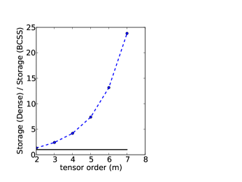
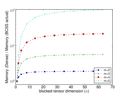
Fig. 5: Actual storage savings of BCSS on 𝓐𝓐\displaystyle\bm{\mathscr{{A}}} with block dimension b𝓐=8subscript𝑏𝓐8\displaystyle b_{\bm{\mathscr{{A}}}}=8. This includes the number of entries required for associated meta-data

As summarized in Table 1, storing only the upper hypertriangular elements of the tensor 𝓐𝓐\displaystyle\bm{\mathscr{{A}}} requires (n+m1m)binomial𝑛𝑚1𝑚\displaystyle\binom{n+m-1}{m} storage, and BCSS requires (n¯+m1m)b𝓐mbinomial¯𝑛𝑚1𝑚superscriptsubscript𝑏𝓐𝑚\displaystyle\binom{\bar{n}+m-1}{m}b_{\bm{\mathscr{{A}}}}^{m} elements which achieves a savings factor of m!𝑚\displaystyle m! (if n¯¯𝑛\displaystyle\bar{n} is large enough).

Although the approximation (n¯+m1m)b𝓐mnmm!binomial¯𝑛𝑚1𝑚superscriptsubscript𝑏𝓐𝑚superscript𝑛𝑚𝑚\displaystyle\binom{\bar{n}+m-1}{m}b_{\bm{\mathscr{{A}}}}^{m}\approx\frac{n^{m}}{m!} is used, the lower-order terms have a significant effect on the actual storage savings factor. In Figure 5, we show the actual storage savings of BCSS (including storage required for meta-data entries) over storing all entries of a symmetric tensor. Examining Figure 5, we see that as we increase m𝑚\displaystyle m, a larger n¯¯𝑛\displaystyle\bar{n} is required to have the actual storage savings factor approach the theoretical factor. While this figure only shows the results for a particular value of b𝓐subscript𝑏𝓐\displaystyle b_{\bm{\mathscr{{A}}}}, the effect applies to all values of b𝓐subscript𝑏𝓐\displaystyle b_{\bm{\mathscr{{A}}}}. This idea of blocking has been used in many projects including the Tensor Contraction Engine (TCE) project [7, 31, 14].

5.4 Algorithm-by-blocks for general m𝑚\displaystyle m

Algorithm Ops Total # of Temp.
(flops) times executed storage
for ȷ¯m1=0,,p¯1subscript¯italic-ȷ𝑚10¯𝑝1\displaystyle\bar{\jmath}_{m-1}=0,\ldots,\bar{p}-1
        𝓣(m1):=𝓐×m1(𝐗ȷ¯m10𝐗ȷ¯m1(n¯1))assignsuperscript𝓣𝑚1subscript𝑚1𝓐subscript𝐗subscript¯italic-ȷ𝑚10subscript𝐗subscript¯italic-ȷ𝑚1¯𝑛1missing-subexpressionmissing-subexpression\displaystyle\bm{\mathscr{{T}}}^{(m-1)}:=\bm{\mathscr{{A}}}\times_{m-1}\left(\begin{array}[]{c c c c c}{\bm{\mathbf{{X}}}}_{\bar{\jmath}_{m-1}0}&\cdots&{\bm{\mathbf{{X}}}}_{\bar{\jmath}_{m-1}(\bar{n}-1)}\end{array}\right) 2b𝓒nm2subscript𝑏𝓒superscript𝑛𝑚\displaystyle 2b_{\bm{\mathscr{{C}}}}n^{m} (p¯1)binomial¯𝑝1\displaystyle\binom{\bar{p}}{1} b𝓒nm1subscript𝑏𝓒superscript𝑛𝑚1\displaystyle b_{\bm{\mathscr{{C}}}}n^{m-1}
           \displaystyle\ddots \displaystyle\vdots \displaystyle\vdots \displaystyle\vdots
           for ȷ¯1=0,,ȷ¯2subscript¯italic-ȷ10subscript¯italic-ȷ2\displaystyle\bar{\jmath}_{1}=0,\ldots,\bar{\jmath}_{2}
                 𝓣(1):=𝓣(2)×1(𝐗ȷ¯10𝐗ȷ¯1(n¯1))assignsuperscript𝓣1subscript1superscript𝓣2subscript𝐗subscript¯italic-ȷ10subscript𝐗subscript¯italic-ȷ1¯𝑛1\displaystyle\bm{\mathscr{{T}}}^{(1)}:=\bm{\mathscr{{T}}}^{(2)}\times_{1}\left(\begin{array}[]{c c c}{\bm{\mathbf{{X}}}}_{\bar{\jmath}_{1}0}&\cdots&{\bm{\mathbf{{X}}}}_{\bar{\jmath}_{1}(\bar{n}-1)}\end{array}\right) 2b𝓒m1n22superscriptsubscript𝑏𝓒𝑚1superscript𝑛2\displaystyle 2b_{\bm{\mathscr{{C}}}}^{m-1}n^{2} (p¯+m2m1)binomial¯𝑝𝑚2𝑚1\displaystyle\binom{\bar{p}+m-2}{m-1} b𝓒m1nsuperscriptsubscript𝑏𝓒𝑚1𝑛\displaystyle b_{\bm{\mathscr{{C}}}}^{m-1}n
                 for ȷ¯0=0,,ȷ¯1subscript¯italic-ȷ00subscript¯italic-ȷ1\displaystyle\bar{\jmath}_{0}=0,\ldots,\bar{\jmath}_{1}
                       𝓒ȷ¯0ȷ¯1ȷ¯m1:=assignsubscript𝓒subscript¯italic-ȷ0subscript¯italic-ȷ1subscript¯italic-ȷ𝑚1absent\displaystyle\bm{\mathscr{{C}}}_{\bar{\jmath}_{0}\bar{\jmath}_{1}\cdots\bar{\jmath}_{m-1}}:=
                           𝓣(1)×0(𝐗ȷ¯00𝐗ȷ¯0(n¯1))=subscript0superscript𝓣1subscript𝐗subscript¯italic-ȷ00subscript𝐗subscript¯italic-ȷ0¯𝑛1absent\displaystyle\bm{\mathscr{{T}}}^{(1)}\times_{0}\left(\begin{array}[]{c c c}{\bm{\mathbf{{X}}}}_{\bar{\jmath}_{0}0}&\cdots&{\bm{\mathbf{{X}}}}_{\bar{\jmath}_{0}(\bar{n}-1)}\end{array}\right)=
                           (𝓣0(1)𝓣n¯1(1))×0(𝐗ȷ¯00𝐗ȷ¯0(n¯1))subscript0subscriptsuperscript𝓣10subscriptsuperscript𝓣1¯𝑛1subscript𝐗subscript¯italic-ȷ00subscript𝐗subscript¯italic-ȷ0¯𝑛1\displaystyle\left(\begin{array}[]{c}\bm{\mathscr{{T}}}^{(1)}_{0}\\ \vdots\\ \bm{\mathscr{{T}}}^{(1)}_{\bar{n}-1}\end{array}\right)\times_{0}\left(\begin{array}[]{c c c}{\bm{\mathbf{{X}}}}_{\bar{\jmath}_{0}0}&\cdots&{\bm{\mathbf{{X}}}}_{\bar{\jmath}_{0}(\bar{n}-1)}\end{array}\right) 2b𝓒mn2superscriptsubscript𝑏𝓒𝑚𝑛\displaystyle 2b_{\bm{\mathscr{{C}}}}^{m}n (p¯+m1m)binomial¯𝑝𝑚1𝑚\displaystyle\binom{\bar{p}+m-1}{m}
                 endfor
           endfor
           \displaystyle\iddots
endfor
Total Cost: d=0m1(2b𝓒d+1nmd(p¯+dd+1)) flopsTotal additional storage: d=0m2(b𝓒d+1nm1d) floatsTotal Cost: superscriptsubscript𝑑0𝑚12superscriptsubscript𝑏𝓒𝑑1superscript𝑛𝑚𝑑binomial¯𝑝𝑑𝑑1 flopsTotal additional storage: superscriptsubscript𝑑0𝑚2superscriptsubscript𝑏𝓒𝑑1superscript𝑛𝑚1𝑑 floats\displaystyle\begin{array}[]{l}\mbox{Total Cost:~{}~{}}\sum_{d=0}^{m-1}\left(2b_{\bm{\mathscr{{C}}}}^{d+1}n^{m-d}\binom{\bar{p}+d}{d+1}\right)\mbox{~{}flops}\\ \mbox{Total additional storage:~{}~{}}\sum_{d=0}^{m-2}\left(b_{\bm{\mathscr{{C}}}}^{d+1}n^{m-1-d}\right)\mbox{~{}floats}\end{array}
Fig. 6: Algorithm-by-blocks for computing 𝓒:=[𝓐;𝐗,,𝐗]assign𝓒𝓐𝐗𝐗\displaystyle\bm{\mathscr{{C}}}:=[\bm{\mathscr{{A}}};{\bm{\mathbf{{X}}}},\cdots,{\bm{\mathbf{{X}}}}]. The algorithm assumes that 𝓒𝓒\displaystyle\bm{\mathscr{{C}}} is partitioned into blocks of size [m,b𝓒]𝑚subscript𝑏𝓒\displaystyle[m,b_{\bm{\mathscr{{C}}}}], with p¯=p/b𝓒¯𝑝𝑝subscript𝑏𝓒\displaystyle\bar{p}=\lceil p/b_{\bm{\mathscr{{C}}}}\rceil.

For 𝓒𝓒\displaystyle\bm{\mathscr{{C}}} and 𝓐𝓐\displaystyle\bm{\mathscr{{A}}} for general m𝑚\displaystyle m stored using BCSS, we discuss how to compute with these blocks. Assume the partioning discussed above. Then,

𝓒ȷ¯0ȷ¯1ȷ¯m1=ı¯0=0n¯1ı¯m1=0n¯1𝓐ı¯0ı¯1ı¯m1×0𝐗ȷ¯0ı¯0×1𝐗ȷ¯1ı¯1×m1𝐗ȷ¯m1ı¯m1=ı¯0=0n¯1ı¯m1=0n¯1[𝓐ı¯0ı¯1ı¯m1;𝐗ȷ¯0ı¯0,𝐗ȷ¯1ı¯1,,𝐗ȷ¯m1ı¯m1].subscript𝓒subscript¯italic-ȷ0subscript¯italic-ȷ1subscript¯italic-ȷ𝑚1absentsuperscriptsubscriptsubscript¯italic-ı00¯𝑛1superscriptsubscriptsubscript¯italic-ı𝑚10¯𝑛1subscript𝑚1subscript1subscript0subscript𝓐subscript¯italic-ı0subscript¯italic-ı1subscript¯italic-ı𝑚1subscript𝐗subscript¯italic-ȷ0subscript¯italic-ı0subscript𝐗subscript¯italic-ȷ1subscript¯italic-ı1subscript𝐗subscript¯italic-ȷ𝑚1subscript¯italic-ı𝑚1missing-subexpressionmissing-subexpressionmissing-subexpressionabsentsuperscriptsubscriptsubscript¯italic-ı00¯𝑛1superscriptsubscriptsubscript¯italic-ı𝑚10¯𝑛1subscript𝓐subscript¯italic-ı0subscript¯italic-ı1subscript¯italic-ı𝑚1subscript𝐗subscript¯italic-ȷ0subscript¯italic-ı0subscript𝐗subscript¯italic-ȷ1subscript¯italic-ı1subscript𝐗subscript¯italic-ȷ𝑚1subscript¯italic-ı𝑚1missing-subexpressionmissing-subexpression\displaystyle\displaystyle\begin{array}[]{r @{\hspace{3pt}} l c l}\bm{\mathscr{{C}}}_{\bar{\jmath}_{0}\bar{\jmath}_{1}\cdots\bar{\jmath}_{m-1}}\hskip 3.0&=\sum_{\bar{\imath}_{0}=0}^{\bar{n}-1}\cdots\sum_{\bar{\imath}_{m-1}=0}^{\bar{n}-1}\bm{\mathscr{{A}}}_{\bar{\imath}_{0}\bar{\imath}_{1}\cdots\bar{\imath}_{m-1}}\times_{0}{\bm{\mathbf{{X}}}}_{\bar{\jmath}_{0}\bar{\imath}_{0}}\times_{1}{\bm{\mathbf{{X}}}}_{\bar{\jmath}_{1}\bar{\imath}_{1}}\cdots\times_{m-1}{\bm{\mathbf{{X}}}}_{\bar{\jmath}_{m-1}\bar{\imath}_{m-1}}\\ \hskip 3.0&=\sum_{\bar{\imath}_{0}=0}^{\bar{n}-1}\cdots\sum_{\bar{\imath}_{m-1}=0}^{\bar{n}-1}[\bm{\mathscr{{A}}}_{\bar{\imath}_{0}\bar{\imath}_{1}\cdots\bar{\imath}_{m-1}};{\bm{\mathbf{{X}}}}_{\bar{\jmath}_{0}\bar{\imath}_{0}},{\bm{\mathbf{{X}}}}_{\bar{\jmath}_{1}\bar{\imath}_{1}},\cdots,{\bm{\mathbf{{X}}}}_{\bar{\jmath}_{m-1}\bar{\imath}_{m-1}}].\end{array}

This yields the algorithm given in Figure 6, which avoids much redundant computation, except for within blocks of 𝓒𝓒\displaystyle\bm{\mathscr{{C}}} that are symmetric or partially symmetric. The algorithm computes temporaries

𝓣(m1)=𝓐×m1𝐗ȷ¯m1:𝓣(m2)=𝓣(m1)×m2𝐗ȷ¯m2:𝓣(1)=𝓣(2)×1𝐗ȷ¯1:superscript𝓣𝑚1subscript𝑚1𝓐subscript𝐗:subscript¯italic-ȷ𝑚1absentsuperscript𝓣𝑚2subscript𝑚2superscript𝓣𝑚1subscript𝐗:subscript¯italic-ȷ𝑚2absentmissing-subexpressionmissing-subexpressionsuperscript𝓣1subscript1superscript𝓣2subscript𝐗:subscript¯italic-ȷ1absent\displaystyle\begin{array}[]{lcl}\bm{\mathscr{{T}}}^{(m-1)}&=&\bm{\mathscr{{A}}}\times_{m-1}{\bm{\mathbf{{X}}}}_{\bar{\jmath}_{m-1}:}\\ \bm{\mathscr{{T}}}^{(m-2)}&=&\bm{\mathscr{{T}}}^{(m-1)}\times_{m-2}{\bm{\mathbf{{X}}}}_{\bar{\jmath}_{m-2}:}\\ &\vdots&\\ \bm{\mathscr{{T}}}^{(1)}&=&\bm{\mathscr{{T}}}^{(2)}\times_{1}{\bm{\mathbf{{X}}}}_{\bar{\jmath}_{1}:}\end{array}

for each index where 0ȷ¯1ȷ¯2ȷ¯m1<p¯0subscript¯italic-ȷ1subscript¯italic-ȷ2subscript¯italic-ȷ𝑚1¯𝑝\displaystyle 0\leq\bar{\jmath}_{1}\leq\bar{\jmath}_{2}\leq\cdots\leq\bar{\jmath}_{m-1}<\bar{p}. This algorithm requires b𝓒nm1+b𝓒2nm2++b𝓒m2nsubscript𝑏𝓒superscript𝑛𝑚1superscriptsubscript𝑏𝓒2superscript𝑛𝑚2superscriptsubscript𝑏𝓒𝑚2𝑛\displaystyle b_{\bm{\mathscr{{C}}}}n^{m-1}+b_{\bm{\mathscr{{C}}}}^{2}n^{m-2}+\cdots+b_{\bm{\mathscr{{C}}}}^{m-2}n extra storage (for 𝓣(m1)superscript𝓣𝑚1\displaystyle\bm{\mathscr{{T}}}^{(m-1)} through 𝓣(1)superscript𝓣1\displaystyle\bm{\mathscr{{T}}}^{(1)}, respectively), in addition to the storage for 𝓒𝓒\displaystyle\bm{\mathscr{{C}}} and 𝓐𝓐\displaystyle\bm{\mathscr{{A}}}.

We realize this approach can result in a small loss of symmetry (due to numerical instability) within blocks. We do not address this effect at this time as the asymmetry only becomes a factor when the resulting tensor is used in subsequent operations. A post-processing step can be applied to correct any asymmetry in the resulting tensor.

6 Exploiting Partial Symmetry

We have shown how to reduce the complexity of the sttsm operation by O(m!)𝑂𝑚\displaystyle O(m!) in terms of storage. In this section, we describe how to achieve the O((m+1)!/2m)𝑂𝑚1superscript2𝑚\displaystyle O((m+1)!/2^{m}) level of reduction in computation.

6.1 Partial Symmetry

Recall that in Figure 6 we utilized a series of temporaries to compute the sttsm operation. To perform the computation, we explicitly formed the temporaries 𝓣(k)superscript𝓣𝑘\displaystyle\bm{\mathscr{{T}}}^{(k)} and did not take advantage of any symmetry in the objects’ entries. Because of this, we were only able to see an O(m)𝑂𝑚\displaystyle O(m) reduction in storage and computation.

However, as we now show, there exists partial symmetry within each temporary that we can exploit to reduce storage and computation as we did for the output tensor 𝓒𝓒\displaystyle\bm{\mathscr{{C}}}. Exploiting this partial symmetry allows the proposed algorithm to match the theoretical reduction in storage and computation.

Theorem 1.

Given an order-m𝑚\displaystyle m tensor 𝓐I0×I1××Im1𝓐superscriptsubscript𝐼0subscript𝐼1subscript𝐼𝑚1\displaystyle\bm{\mathscr{{A}}}\in\mathbb{R}^{I_{0}\times I_{1}\times\cdots\times I_{m-1}} that has modes 00\displaystyle 0 through k𝑘\displaystyle k symmetric (thus I0=I1==Iksubscript𝐼0subscript𝐼1subscript𝐼𝑘\displaystyle I_{0}=I_{1}=\cdots=I_{k}), then 𝓒=𝓐×k𝐗𝓒subscript𝑘𝓐𝐗\displaystyle\bm{\mathscr{{C}}}=\bm{\mathscr{{A}}}\times_{k}{\bm{\mathbf{{X}}}} has modes 00\displaystyle 0 through k1𝑘1\displaystyle k-1 symmetric.

Proof.

We prove this by construction of 𝓒𝓒\displaystyle\bm{\mathscr{{C}}}.

Since 𝓐𝓐\displaystyle\bm{\mathscr{{A}}} has modes 00\displaystyle 0 through k𝑘\displaystyle k symmetric, we know (from Section 2.4) that

αi0i1ikik+1im1=αi0i1ikik+1im1subscript𝛼superscriptsubscript𝑖0superscriptsubscript𝑖1superscriptsubscript𝑖𝑘subscript𝑖𝑘1subscript𝑖𝑚1subscript𝛼subscript𝑖0subscript𝑖1subscript𝑖𝑘subscript𝑖𝑘1subscript𝑖𝑚1\displaystyle\alpha_{i_{0}^{\prime}i_{1}^{\prime}\cdots i_{k}^{\prime}i_{k+1}\cdots i_{m-1}}=\alpha_{i_{0}i_{1}\cdots i_{k}i_{k+1}\cdots i_{m-1}}

under the relevent permutations. We wish to show that

γi0i1ik1jkjm1=γi0i1ik1jkjm1subscript𝛾superscriptsubscript𝑖0superscriptsubscript𝑖1superscriptsubscript𝑖𝑘1subscript𝑗𝑘subscript𝑗𝑚1subscript𝛾subscript𝑖0subscript𝑖1subscript𝑖𝑘1subscript𝑗𝑘subscript𝑗𝑚1\displaystyle\gamma_{i_{0}^{\prime}i_{1}^{\prime}\cdots i_{k-1}^{\prime}j_{k}\cdots j_{m-1}}=\gamma_{i_{0}i_{1}\cdots i_{k-1}j_{k}\cdots j_{m-1}}

for all indices in 𝓒𝓒\displaystyle\bm{\mathscr{{C}}}.

γi0i1ik1jkjm1==0n1αi0i1ik1jk+1jm1χjk==0n1αi0i1ik1jk+1jm1χjk=γi0i1ik1jkjm1.subscript𝛾superscriptsubscript𝑖0superscriptsubscript𝑖1superscriptsubscript𝑖𝑘1subscript𝑗𝑘subscript𝑗𝑚1superscriptsubscript0𝑛1subscript𝛼superscriptsubscript𝑖0superscriptsubscript𝑖1superscriptsubscript𝑖𝑘1subscript𝑗𝑘1subscript𝑗𝑚1subscript𝜒subscript𝑗𝑘missing-subexpressionmissing-subexpressionmissing-subexpressionsuperscriptsubscript0𝑛1subscript𝛼subscript𝑖0subscript𝑖1subscript𝑖𝑘1subscript𝑗𝑘1subscript𝑗𝑚1subscript𝜒subscript𝑗𝑘subscript𝛾subscript𝑖0subscript𝑖1subscript𝑖𝑘1subscript𝑗𝑘subscript𝑗𝑚1\displaystyle\begin{array}[]{l c l c l}\gamma_{i_{0}^{\prime}i_{1}^{\prime}\cdots i_{k-1}^{\prime}j_{k}\cdots j_{m-1}}&=&\sum_{\ell=0}^{n-1}\alpha_{i_{0}^{\prime}i_{1}^{\prime}\cdots i_{k-1}^{\prime}\ell j_{k+1}\cdots j_{m-1}}\chi_{j_{k}\ell}&&\\ &=&\sum_{\ell=0}^{n-1}\alpha_{i_{0}i_{1}\cdots i_{k-1}\ell j_{k+1}\cdots j_{m-1}}\chi_{j_{k}\ell}&=&\gamma_{i_{0}i_{1}\cdots i_{k-1}j_{k}\cdots j_{m-1}}.\\ \end{array}

Since γi0i1ik1jkjm1=γi0i1ik1jkjm1subscript𝛾superscriptsubscript𝑖0superscriptsubscript𝑖1superscriptsubscript𝑖𝑘1subscript𝑗𝑘subscript𝑗𝑚1subscript𝛾subscript𝑖0subscript𝑖1subscript𝑖𝑘1subscript𝑗𝑘subscript𝑗𝑚1\displaystyle\gamma_{i_{0}^{\prime}i_{1}^{\prime}\cdots i_{k-1}^{\prime}j_{k}\cdots j_{m-1}}=\gamma_{i_{0}i_{1}\cdots i_{k-1}j_{k}\cdots j_{m-1}} for all indices in 𝓒𝓒\displaystyle\bm{\mathscr{{C}}}, we can say that 𝓒𝓒\displaystyle\bm{\mathscr{{C}}} has modes 00\displaystyle 0 through k1𝑘1\displaystyle k-1 symmetric. ∎

By applying Theorem 1 to the algorithm in Figure 6, we observe that all temporaries of the form 𝓣(k)superscript𝓣𝑘\displaystyle\bm{\mathscr{{T}}}^{(k)} formed have modes 00\displaystyle 0 through k1𝑘1\displaystyle k-1 symmetric. It is this partial symmetry we exploit to further reduce storage and computational complexityIt is true that the other modes may have symmetry as well, however in general this is not the case, and therefore we do not explore exploiting this symmetry.

6.2 Storage

A generalization of the BCSS scheme can be applied to the partially symmetric temporary tensors as well. To do this, we view each temporary tensor as being comprised of a group of symmetric modes and a group of non-symmetric modes. There is once again opportunity for storage savings as the symmetric indices have redundancies. As in the BCSS case for symmetric tensors, unique blocks are stored and meta-data indicating how to transform stored blocks to the corresponding block is stored for all redundant block entries.

6.3 Computation

Recall that each temporary is computed via
𝓣(k)=𝓣(k+1)×k+1𝐁superscript𝓣𝑘subscript𝑘1superscript𝓣𝑘1𝐁\displaystyle\bm{\mathscr{{T}}}^{(k)}=\bm{\mathscr{{T}}}^{(k+1)}\times_{k+1}{\bm{\mathbf{{B}}}} where 𝓣(k)superscript𝓣𝑘\displaystyle\bm{\mathscr{{T}}}^{(k)} and 𝓣(k+1)superscript𝓣𝑘1\displaystyle\bm{\mathscr{{T}}}^{(k+1)} have associated symmetries (𝓣(m)=𝓐superscript𝓣𝑚𝓐\displaystyle\bm{\mathscr{{T}}}^{(m)}=\bm{\mathscr{{A}}} when computing 𝓣(m1)superscript𝓣𝑚1\displaystyle\bm{\mathscr{{T}}}^{(m-1)}), and 𝐁𝐁\displaystyle{\bm{\mathbf{{B}}}} is some matrix. We can rewrite this operation as:

𝓣(k)=𝓣(k+1)×k+1𝐁=𝓣(k+1)×0𝐈×1×k𝐈×k+1𝐁×k+2𝐈×k+3×m1𝐈,superscript𝓣𝑘subscript𝑘1superscript𝓣𝑘1𝐁subscript𝑚1subscript𝑘3subscript𝑘2subscript𝑘1subscript𝑘subscript1subscript0superscript𝓣𝑘1𝐈𝐈𝐁𝐈𝐈\displaystyle\begin{array}[]{l c l}\bm{\mathscr{{T}}}^{(k)}&=&\bm{\mathscr{{T}}}^{(k+1)}\times_{k+1}{\bm{\mathbf{{B}}}}=\bm{\mathscr{{T}}}^{(k+1)}\times_{0}{\bm{\mathbf{{I}}}}\times_{1}\cdots\times_{k}{\bm{\mathbf{{I}}}}\times_{k+1}{\bm{\mathbf{{B}}}}\times_{k+2}{\bm{\mathbf{{I}}}}\times_{k+3}\cdots\times_{m-1}{\bm{\mathbf{{I}}}},\\ \end{array}

where 𝐈𝐈\displaystyle{\bm{\mathbf{{I}}}} is the first p𝑝\displaystyle p rows of the n×n𝑛𝑛\displaystyle n\times n identity matrix. An algorithm akin to that of Figure 6 can be created (care is taken to only update unique output blocks) to perform the necessary computation. Of course, computing with the identity matrix is wasteful, and therefore, we only implicitly compute with the identity matrix to save on computation.

6.4 Analysis

BCSS Dense
𝓐𝓐\displaystyle\bm{\mathscr{{A}}}
(elements)
b𝓐m(n¯+m1m)+n¯msuperscriptsubscript𝑏𝓐𝑚binomial¯𝑛𝑚1𝑚superscript¯𝑛𝑚\displaystyle b_{\bm{\mathscr{{A}}}}^{m}\binom{\bar{n}+m-1}{m}+\bar{n}^{m} nmsuperscript𝑛𝑚\displaystyle n^{m}
𝓒𝓒\displaystyle\bm{\mathscr{{C}}}
(elements)
b𝓒m(p¯+m1m)+p¯msuperscriptsubscript𝑏𝓒𝑚binomial¯𝑝𝑚1𝑚superscript¯𝑝𝑚\displaystyle b_{\bm{\mathscr{{C}}}}^{m}\binom{\bar{p}+m-1}{m}+\bar{p}^{m} pmsuperscript𝑝𝑚\displaystyle p^{m}
𝐗𝐗\displaystyle{\bm{\mathbf{{X}}}}
(elements)
pn𝑝𝑛\displaystyle pn pn𝑝𝑛\displaystyle pn
All temporaries
(elements)
b𝓒b𝓐m1d=0m2((n¯+md2md1)(b𝓒b𝓐)d+n¯d+1)subscript𝑏𝓒superscriptsubscript𝑏𝓐𝑚1superscriptsubscript𝑑0𝑚2binomial¯𝑛𝑚𝑑2𝑚𝑑1superscriptsubscript𝑏𝓒subscript𝑏𝓐𝑑superscript¯𝑛𝑑1\displaystyle b_{\bm{\mathscr{{C}}}}b_{\bm{\mathscr{{A}}}}^{m-1}\sum_{d=0}^{m-2}\left(\binom{\bar{n}+m-d-2}{m-d-1}\left(\frac{b_{\bm{\mathscr{{C}}}}}{b_{\bm{\mathscr{{A}}}}}\right)^{d}+\bar{n}^{d+1}\right) pnm1d=0m2(pn)d𝑝superscript𝑛𝑚1superscriptsubscript𝑑0𝑚2superscript𝑝𝑛𝑑\displaystyle pn^{m-1}\sum_{d=0}^{m-2}\left(\frac{p}{n}\right)^{d}
Computation
(flops)
2n¯b𝓒b𝓐md=0m1(p¯+dd+1)(n¯+md2md1)(b𝓒b𝓐)d2¯𝑛subscript𝑏𝓒superscriptsubscript𝑏𝓐𝑚superscriptsubscript𝑑0𝑚1binomial¯𝑝𝑑𝑑1binomial¯𝑛𝑚𝑑2𝑚𝑑1superscriptsubscript𝑏𝓒subscript𝑏𝓐𝑑\displaystyle 2\bar{n}b_{\bm{\mathscr{{C}}}}b_{\bm{\mathscr{{A}}}}^{m}\sum_{d=0}^{m-1}\binom{\bar{p}+d}{d+1}\binom{\bar{n}+m-d-2}{m-d-1}\left(\frac{b_{\bm{\mathscr{{C}}}}}{b_{\bm{\mathscr{{A}}}}}\right)^{d} 2pnmd=0m1(pn)d2𝑝superscript𝑛𝑚superscriptsubscript𝑑0𝑚1superscript𝑝𝑛𝑑\displaystyle 2pn^{m}\sum_{d=0}^{m-1}\left(\frac{p}{n}\right)^{d}
Permutation
(memops)
(n¯+2b𝓒b𝓐)b𝓐md=0m1(p¯+dd+1)(n¯+md2md1)(b𝓒b𝓐)d¯𝑛2subscript𝑏𝓒subscript𝑏𝓐superscriptsubscript𝑏𝓐𝑚superscriptsubscript𝑑0𝑚1binomial¯𝑝𝑑𝑑1binomial¯𝑛𝑚𝑑2𝑚𝑑1superscriptsubscript𝑏𝓒subscript𝑏𝓐𝑑\displaystyle\left(\bar{n}+2\frac{b_{\bm{\mathscr{{C}}}}}{b_{\bm{\mathscr{{A}}}}}\right)b_{\bm{\mathscr{{A}}}}^{m}\sum_{d=0}^{m-1}\binom{\bar{p}+d}{d+1}\binom{\bar{n}+m-d-2}{m-d-1}\left(\frac{b_{\bm{\mathscr{{C}}}}}{b_{\bm{\mathscr{{A}}}}}\right)^{d} (1+2pn)nmd=0m1(pn)d12𝑝𝑛superscript𝑛𝑚superscriptsubscript𝑑0𝑚1superscript𝑝𝑛𝑑\displaystyle\left(1+2\frac{p}{n}\right)n^{m}\sum_{d=0}^{m-1}\left(\frac{p}{n}\right)^{d}
Table 2: Costs associated with different algorithms for computing 𝓒=[𝓐;𝐗,,𝐗]𝓒𝓐𝐗𝐗\displaystyle\bm{\mathscr{{C}}}=[\bm{\mathscr{{A}}};{\bm{\mathbf{{X}}}},\ldots,{\bm{\mathbf{{X}}}}]. The BCSS column takes advantage of partial-symmetry within the temporaries. The n¯msuperscript¯𝑛𝑚\displaystyle\bar{n}^{m}, p¯msuperscript¯𝑝𝑚\displaystyle\bar{p}^{m}, and n¯d+1superscript¯𝑛𝑑1\displaystyle\bar{n}^{d+1} terms correspond to the number of meta-data elements associated with our choice of storage scheme.

Utilizing this optimization allows us to arrive at the final cost functions for storage and computation shown in Table 2.

Taking, for example, the computational cost (assuming n=p𝑛𝑝\displaystyle n=p and b𝓐=b𝓒subscript𝑏𝓐subscript𝑏𝓒\displaystyle b_{\bm{\mathscr{{A}}}}=b_{\bm{\mathscr{{C}}}}), we have the following expression for the cost of the BCSS algorithm:

2n¯b𝓒b𝓐md=0m1(p¯+dd+1)(n¯+md2md1)(b𝓒b𝓐)d=2nb𝓐md=0m1(n¯+dd+1)(n¯+m(d+1)1m(d+1))(1)d2nb𝓐m(2n¯+m2m)2nb𝓐m(2n¯)mm!=(2n)m+1m!.2n¯b𝓒b𝓐md=0m1(p¯+dd+1)(n¯+md2md1)(b𝓒b𝓐)dmissing-subexpression2𝑛superscriptsubscript𝑏𝓐𝑚superscriptsubscript𝑑0𝑚1binomial¯𝑛𝑑𝑑1binomial¯𝑛𝑚𝑑11𝑚𝑑1superscript1𝑑missing-subexpressionmissing-subexpressionmissing-subexpressionmissing-subexpression2𝑛superscriptsubscript𝑏𝓐𝑚binomial2¯𝑛𝑚2𝑚2𝑛superscriptsubscript𝑏𝓐𝑚superscript2¯𝑛𝑚𝑚superscript2𝑛𝑚1𝑚\displaystyle\begin{array}[]{lcl}\lx@intercol\@ADDCLASS{ltx_eqn_lefteqn}$\displaystyle\displaystyle 2\bar{n}b_{\bm{\mathscr{{C}}}}b_{\bm{\mathscr{{A}}}}^{m}\sum_{d=0}^{m-1}\binom{\bar{p}+d}{d+1}\binom{\bar{n}+m-d-2}{m-d-1}\left(\frac{b_{\bm{\mathscr{{C}}}}}{b_{\bm{\mathscr{{A}}}}}\right)^{d}$\mbox{}\hfil\lx@intercol\\ &=&2nb_{\bm{\mathscr{{A}}}}^{m}\sum_{d=0}^{m-1}\binom{\bar{n}+d}{d+1}\binom{\bar{n}+m-(d+1)-1}{m-(d+1)}\left(1\right)^{d}\\ &&\\ &\approx&2nb_{\bm{\mathscr{{A}}}}^{m}\binom{2\bar{n}+m-2}{m}\approx 2nb_{\bm{\mathscr{{A}}}}^{m}\frac{\left(2\bar{n}\right)^{m}}{m!}=\frac{\left(2n\right)^{m+1}}{m!}.\\ \end{array}

To achieve this approximation, the Vandermonde identity, which states that

(m+nr)=k=0r(mk)(nrk)binomial𝑚𝑛𝑟superscriptsubscript𝑘0𝑟binomial𝑚𝑘binomial𝑛𝑟𝑘\displaystyle\binom{m+n}{r}=\sum_{k=0}^{r}\binom{m}{k}\binom{n}{r-k}

was employed.

BCSS Dense
𝓐𝓐\displaystyle\bm{\mathscr{{A}}}, 𝓒𝓒\displaystyle\bm{\mathscr{{C}}}
(elements)
b𝓐m(n¯+m1m)superscriptsubscript𝑏𝓐𝑚binomial¯𝑛𝑚1𝑚\displaystyle b_{\bm{\mathscr{{A}}}}^{m}\binom{\bar{n}+m-1}{m} nmsuperscript𝑛𝑚\displaystyle n^{m}
𝐗𝐗\displaystyle{\bm{\mathbf{{X}}}}
(elements)
n2superscript𝑛2\displaystyle n^{2} n2superscript𝑛2\displaystyle n^{2}
All temporaries
(elements)
nmm!superscript𝑛𝑚𝑚\displaystyle\frac{n^{m}}{m!} (m1)nm𝑚1superscript𝑛𝑚\displaystyle(m-1)n^{m}
Computation
(flops)
(2n)m+1m!superscript2𝑛𝑚1𝑚\displaystyle\frac{(2n)^{m+1}}{m!} 2mnm+12𝑚superscript𝑛𝑚1\displaystyle 2mn^{m+1}
Permutation
(memops)
(n¯+2)(2n)mm!¯𝑛2superscript2𝑛𝑚𝑚\displaystyle(\bar{n}+2)\frac{(2n)^{m}}{m!} 3mnm3𝑚superscript𝑛𝑚\displaystyle 3mn^{m}
Table 3: Approximate costs associated with different algorithms for computing 𝓒=[𝓐;𝐗,,𝐗]𝓒𝓐𝐗𝐗\displaystyle\bm{\mathscr{{C}}}=[\bm{\mathscr{{A}}};{\bm{\mathbf{{X}}}},\ldots,{\bm{\mathbf{{X}}}}]. The BCSS column takes advantage of partial symmetry within the temporaries. In the above costs, it is assumed that the tensor dimensions and block dimensions of 𝓐𝓐\displaystyle\bm{\mathscr{{A}}} and 𝓒𝓒\displaystyle\bm{\mathscr{{C}}} are equal, i.e. n=p𝑛𝑝\displaystyle n=p and b𝓐=b𝓒subscript𝑏𝓐subscript𝑏𝓒\displaystyle b_{\bm{\mathscr{{A}}}}=b_{\bm{\mathscr{{C}}}}. We assume nm>>n¯mmuch-greater-thansuperscript𝑛𝑚superscript¯𝑛𝑚\displaystyle n^{m}>>\bar{n}^{m}.

Using similar approximations, we arrive at the estimates summarized in Table 3.

Comparing this computational cost to that of the Dense algorithm (as given in Table 3), we see that the BCSS algorithm achieves a reduction of

Dense costBCSS cost=2mnm+1((2n)m+1m!)(m+1)!2m Dense costBCSS cost2𝑚superscript𝑛𝑚1superscript2𝑛𝑚1𝑚𝑚1superscript2𝑚 \displaystyle\frac{\text{Dense cost}}{\text{BCSS cost}}=\frac{2mn^{m+1}}{\left(\frac{(2n)^{m+1}}{m!}\right)}\approx\frac{(m+1)!}{2^{m}}\text{ }

in terms of computation.

6.5 Analysis relative to minimum

As we are storing some elements redundantly, it is important to compare how the algorithm performs compared to the case where we store no extra elements, that is, we only compute the unique entries of 𝓒𝓒\displaystyle\bm{\mathscr{{C}}}. Assuming 𝓐[m,n]𝓐superscript𝑚𝑛\displaystyle\bm{\mathscr{{A}}}\in\mathbb{R}^{[m,n]}, 𝓒[m,p]𝓒superscript𝑚𝑝\displaystyle\bm{\mathscr{{C}}}\in\mathbb{R}^{[m,p]}, p=n𝑝𝑛\displaystyle p=n, and b𝓐=b𝓒=1subscript𝑏𝓐subscript𝑏𝓒1\displaystyle b_{\bm{\mathscr{{A}}}}=b_{\bm{\mathscr{{C}}}}=1, the cost of computing the sttsm operation is

2nd=0m1(n+dd+1)(n+md2md1)2n(2n+m2m)2n(2n)mm!=(2n)m+1m!,2𝑛superscriptsubscript𝑑0𝑚1binomial𝑛𝑑𝑑1binomial𝑛𝑚𝑑2𝑚𝑑12𝑛binomial2𝑛𝑚2𝑚2𝑛superscript2𝑛𝑚𝑚superscript2𝑛𝑚1𝑚\displaystyle 2n\sum_{d=0}^{m-1}\binom{n+d}{d+1}\binom{n+m-d-2}{m-d-1}\approx 2n\binom{2n+m-2}{m}\approx 2n\frac{(2n)^{m}}{m!}=\frac{(2n)^{m+1}}{m!},

which is of the same order as our blocked algorithm.

6.6 Summary
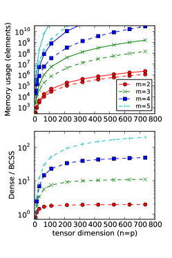
Refer to caption Refer to caption Refer to caption
Fig. 7: Comparison of Dense to BCSS algorithms for fixed block size. Solid and dashed lines correspond to Dense and BCSS, respectively. From left to right: storage requirements, cost from computation (flops), cost from permutations (memops). For these graphs b𝓐=b𝓒=8subscript𝑏𝓐subscript𝑏𝓒8\displaystyle b_{\bm{\mathscr{{A}}}}=b_{\bm{\mathscr{{C}}}}=8.
Refer to caption Refer to caption Refer to caption
Fig. 8: Comparison of Dense to BCSS algorithms for fixed number of blocks. Solid and dashed lines correspond to Dense and BCSS, respectively. From left to right: storage requirements, cost from computation (flops), cost from permutations (memops). Here n¯=p¯=2¯𝑛¯𝑝2\displaystyle\bar{n}=\bar{p}=2.

Figures 88 illustrate the insights discussed in this section. The (exact) formulae developed for storage, flops, and memops are used to compare and contrast dense storage with BCSS.

In Figure 8, the top graphs report storage, flops, and memops (due to permutations) as a function of tensor dimension (n𝑛\displaystyle n), for different tensor orders (m𝑚\displaystyle m), for the case where the storage block size is relatively small (b𝓐=b𝓒=8subscript𝑏𝓐subscript𝑏𝓒8\displaystyle b_{\bm{\mathscr{{A}}}}=b_{\bm{\mathscr{{C}}}}=8). The bottom graphs report the same information, but as a ratio. The graphs illustrate that BCSS dramatically reduces the required storage and the proposed algorithms reduce the flops requirements for the sttsm operation, at the expense of additional memops due to the encountered permutations.

In Figure 8, a similar analysis is given, but for the case where the block size is half the tensor dimension (i.e., n¯=p¯=2¯𝑛¯𝑝2\displaystyle\bar{n}=\bar{p}=2). It shows that the memops can be greatly reduced by increasing the storage block dimensions, but this then adversely affects the storage and computational benefits.

It would be tempting to discuss how to choose an optimal block dimension. However, the real issue is that the overhead of permutation should be reduced and/or eliminated. Once that is achieved, in future research, the question of how to choose the block size becomes relevant.

7 Experimental Results

In this section, we report on the performance attained by an implementation of the discussed approach. It is important to keep in mind that the current state of the art of tensor computations is first and foremost concerned with reducing memory requirements so that reasonably large problems can be executed. This is where taking advantage of symmetry is important. With that said, another primary concern is ensuring the overall time of computation is reduced. To achieve this, a reduction in the number of floating point operations as well as an implementation that computes the necessary operations efficiently are both desired. Second to that is the desire to reduce the number of floating point operations to the minimum required. The provided analysis shows that our algorithms perform the minimum number of floating point operations (under approximation). Although our algorithms do not yet perform these operations efficiently, our results show that we are still able to reduce the computation time (in some cases significantly).

7.1 Target architecture

We report on experiments on a single core of a Dell PowerEdge R900 server consisting of four six-core Intel Xeon 7400 processors and 96 GBytes of memory. Performance experiments were gathered under the GNU/Linux 2.6.18 operating system. Source code was compiled by the GNU C compiler, version 4.1.2. All experiments were performed in double-precision floating-point arithmetic on randomized real domain matrices and tensors. The implementations were linked to the OpenBLAS 0.1.1 library [1, 39], a fork of the GotoBLAS2 implementation of the BLAS [17, 16]. As noted, most time is spent in the permutations necessary to cast computation in terms of the BLAS matrix-matrix multiplication routine dgemm. Thus, the peak performance of the processor and the details of the performance attained by the BLAS library are mostly irrelevant at this stage. The experiments merely show that the new approach to storing matrices as well as the algorithm that takes advantage of symmetry has promise, rather than making a statement about optimality of the implementation. For instance, as argued previously, we know that tensor permutations can dominate the time spent computing the sttsm operation. These experiments make no attempt to reduce the number of tensor permutations required when computing a single block of the output. Algorithms reducing the effect of tensor permutations have been specialized for certain tensor operations and have been shown to greatly increase the performance of routines using them [26, 34]. Much room for improvement remains.

7.2 Implementation

The implementation was coded in a style inspired by the libflame library [41, 36] and can be found in the Google Code tlash project (code.google.com/p/tlash). An API similar to the FLASH API [24] for storing matrices as matrices of blocks and implementing algorithm-by-blocks was defined and implemented. Computations with the (tensor and matrix) blocks were implemented as the discussed sequence of permutations interleaved with calls to the dgemm BLAS kernel. No attempt was yet made to optimize these permutations. However, an apples-to-apples comparison resulted from using the same sequence of permutations and calls to dgemm for both the experiments that take advantage of symmetry and those that store and compute with the tensor densely, ignoring symmetry.
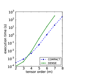
Refer to caption Refer to caption Refer to caption
Fig. 9: Experimental results when n=p=16𝑛𝑝16\displaystyle n=p=16, b𝓐=b𝓒=8subscript𝑏𝓐subscript𝑏𝓒8\displaystyle b_{\bm{\mathscr{{A}}}}=b_{\bm{\mathscr{{C}}}}=8 and the tensor order, m𝑚\displaystyle m, is varied. For m=8𝑚8\displaystyle m=8, storing 𝓐𝓐\displaystyle\bm{\mathscr{{A}}} and 𝓒𝓒\displaystyle\bm{\mathscr{{C}}} without taking advantage of symmetry requires too much memory. The solid black line is used to indicate a unit ratio.
Refer to caption Refer to caption Refer to caption
Fig. 10: Experimental results when the order m=5𝑚5\displaystyle m=5, b𝓐=b𝓒=8subscript𝑏𝓐subscript𝑏𝓒8\displaystyle b_{\bm{\mathscr{{A}}}}=b_{\bm{\mathscr{{C}}}}=8 and the tensor dimensions n=p𝑛𝑝\displaystyle n=p are varied. For n=p=72𝑛𝑝72\displaystyle n=p=72, storing 𝓐𝓐\displaystyle\bm{\mathscr{{A}}} and 𝓒𝓒\displaystyle\bm{\mathscr{{C}}} without taking advantage of symmetry requires too much memory. The solid black line is used to indicate a unit ratio.
Refer to caption Refer to caption Refer to caption
Fig. 11: Experimental results when the order m=5𝑚5\displaystyle m=5, n=p=64𝑛𝑝64\displaystyle n=p=64 and the block dimensions b𝓐=b𝓒subscript𝑏𝓐subscript𝑏𝓒\displaystyle b_{\bm{\mathscr{{A}}}}=b_{\bm{\mathscr{{C}}}} are varied. The solid black line is used to indicate a unit ratio.
Refer to caption Refer to caption Refer to caption
Fig. 12: Experimental results when the order m=3𝑚3\displaystyle m=3, n=p=1000𝑛𝑝1000\displaystyle n=p=1000 and the block dimensions b𝓐=b𝓒subscript𝑏𝓐subscript𝑏𝓒\displaystyle b_{\bm{\mathscr{{A}}}}=b_{\bm{\mathscr{{C}}}} are varied. The solid black line is used to indicate a unit ratio.
Refer to caption
Fig. 13: Comparison of computational cost to permutation cost where m=5𝑚5\displaystyle m=5, n=p=64𝑛𝑝64\displaystyle n=p=64 and tensor block dimension (b𝓐subscript𝑏𝓐\displaystyle b_{\bm{\mathscr{{A}}}}, b𝓒subscript𝑏𝓒\displaystyle b_{\bm{\mathscr{{C}}}}) is varied. The solid line represents the number of flops (due to computation) required for a given problem (left axis), and the dashed line represents the number of memops (due to permutation) required for a given problem (right axis).

7.3 Results

Figures 912 show results from executing our implementation on the target architecture. The Dense algorithm does not take advantage of symmetry nor blocking of the data objects, whereas the BCSS algorithm takes advantage of both. All figures show comparisons of the execution time of each algorithm, the associated speedup of the BCSS algorithm over the Dense algorithm, and the estimated storage savings factor of the BCSS algorithm not including storage required for meta-data.

For the experiments reported in Figure 9 we fix the dimensions n𝑛\displaystyle n and p𝑝\displaystyle p, and the block-sizes b𝓐subscript𝑏𝓐\displaystyle b_{\bm{\mathscr{{A}}}} and b𝓒subscript𝑏𝓒\displaystyle b_{\bm{\mathscr{{C}}}}, and vary the tensor order m𝑚\displaystyle m. Based on experiment, the BCSS algorithm begins to outperform the Dense algorithm after the tensor order is greater than or equal to 44\displaystyle 4. This effect for small m𝑚\displaystyle m should be understood in context of the experiments performed. As n=p=16𝑛𝑝16\displaystyle n=p=16, the problem size is quite small (the problem for m=2𝑚2\displaystyle m=2 and m=3𝑚3\displaystyle m=3 are equivalent to a matrices of size 16×161616\displaystyle 16\times 16 and 64×646464\displaystyle 64\times 64 respectively) reducing the benefit of storage-by-blocks (as storing the entire matrix contiguously requires minor space overhead but benefits greatly from more regular data access). Since such small problems do not provide useful comparisons for the reader, the results of using the BCSS algorithm with problem parameters m=3𝑚3\displaystyle m=3, n=p=1000𝑛𝑝1000\displaystyle n=p=1000, and varied block-dimensions are given in Figure 12. Figure 12 shows that the BCSS algorithm is able to outperform the Dense algorithm given a large enough problem size and an appropriate block size. Additionally, notice that BCSS allows larger problems to be solved; the Dense algorithm was unable to compute the result when an order-88\displaystyle 8 tensor was given as input due to an inability to store the problem in memory.

Our model predicts that the BCSS algorithm should achieve an O((m+1)!/2m)𝑂𝑚1superscript2𝑚\displaystyle O\left((m+1)!/2^{m}\right) speedup over the Dense algorithm. Although it appears that our experiments are only achieving a linear speedup over the Dense algorithm, this is because the values of m𝑚\displaystyle m are so small that the predicted speedup factor is approximately linear with respect to m𝑚\displaystyle m. In terms of storage savings, we would expect the BCSS algorithm to have an O(m!)𝑂𝑚\displaystyle O\left(m!\right) reduction in space over the Dense algorithm. The fact that we are not seeing this in the experiments is because the block dimensions b𝓐subscript𝑏𝓐\displaystyle b_{\bm{\mathscr{{A}}}} and b𝓒subscript𝑏𝓒\displaystyle b_{\bm{\mathscr{{C}}}} are relatively large when compared to the tensor dimensions n𝑛\displaystyle n and p𝑝\displaystyle p meaning the BCSS algorithm does not have as great an opportunity to reduce storage requirements.

In Figure 11 we fix the order m𝑚\displaystyle m, the block-sizes b𝓐subscript𝑏𝓐\displaystyle b_{\bm{\mathscr{{A}}}}, and b𝓒subscript𝑏𝓒\displaystyle b_{\bm{\mathscr{{C}}}} and vary the tensor dimensions n𝑛\displaystyle n and p𝑝\displaystyle p. We see that the BCSS algorithm outperforms the Dense algorithm and attains a noticeable speedup. The experiments show a roughly linear speedup when viewed relative to n𝑛\displaystyle n with perhaps a slight leveling off effect towards larger problem dimensions. We would expect the BCSS algorithm to approach a maximum speedup relative to the Dense algorithm. According to Figure 8, we would expect the speedup of the BCSS algorithm over the Dense algorithm to level off completely when our problem dimensions (n𝑛\displaystyle n and p𝑝\displaystyle p) are on the order of 400400\displaystyle 400 to 600600\displaystyle 600. Unfortunately, due to space limitations we were unable to test beyond the n=p=64𝑛𝑝64\displaystyle n=p=64 problem dimension and therefore were unable to completely observe the leveling off effect in the speedup.

In Figure 11 we fix m𝑚\displaystyle m, n𝑛\displaystyle n, and p𝑝\displaystyle p, and vary the block sizes b𝓐subscript𝑏𝓐\displaystyle b_{\bm{\mathscr{{A}}}} and b𝓒subscript𝑏𝓒\displaystyle b_{\bm{\mathscr{{C}}}}. The right-most point on the axis corresponds to the dense case (as b𝓐=n=b𝓒=psubscript𝑏𝓐𝑛subscript𝑏𝓒𝑝\displaystyle b_{\bm{\mathscr{{A}}}}=n=b_{\bm{\mathscr{{C}}}}=p) and the left-most point corresponds to the fully-compact case (where only unique entries are stored). There now is a range of block dimensions for which the BCSS algorithm outperforms the Dense algorithm. Further, the BCSS algorithm performs as well or worse than the Dense counterpart at the two endpoints in the graph. This is expected toward the right of the figure as the BCSS algorithm reduces to the Dense algorithm, however the left of the figure requires a different explanation.

In Figure 13, we illustrate (with predicted flop and memop counts) that there exists a point where smaller block dimensions dramatically increases the number of memops required to compute the operation. Although a smaller block dimension results in less flops required for computing, the number of memops required increases significantly more. As memops are typically significantly more expensive than flops, we can expect that picking too small a block dimension can be expected to drastically degrade overall performance.

8 Conclusion and Future Work

We present storage by blocks, BCSS, for tensors and show how this can be used to compactly store symmetric tensors. The benefits are demonstrated with an implementation of a new algorithm for the change-of-basis (sttsm) operation. Theoretical and practical results show that both the storage and computational requirements are reduced relative to storing the tensors densely and computing without taking advantage of symmetry.

This initial study exposes many new research opportunities for extending insights from the field of high-performance linear algebra to multi-linear computation, which we believe to be the real contribution of this paper. We finish by discussing some of these opportunities.

Optimizing tensor permutations

In our work, we made absolutely no attempt to optimize the tensor permutation operation. Without doubt, a careful study of how to organize these tensor permutations will greatly benefit performance. It is likely that the current implementation not only causes unnecessary cache misses, but also a great number of Translation Lookaside Buffer (TLB) misses [17], which cause the core to stall for a hundred or more cycles.

Optimized kernels/avoiding tensor permutations

A better way to mitigate the tensor permutations is to avoid them as much as possible. If n=p𝑛𝑝\displaystyle n=p, the sttsm operation performs O(nm+1)𝑂superscript𝑛𝑚1\displaystyle O(n^{m+1}) operations on O(nm)𝑂superscript𝑛𝑚\displaystyle O(n^{m}) data. This exposes plenty of opportunity to optimize this kernel much like dgemm, which performs O(n3)𝑂superscript𝑛3\displaystyle O(n^{3}) computation on O(n2)𝑂superscript𝑛2\displaystyle O(n^{2}) data, is optimized. For other tensor operations, the ratio is even more favorable.

We are developing a BLAS-like library, BLIS [37], that allows matrix operations with matrices that have both a row and a column stride, as opposed to the traditional column-major order supported by the BLAS. This means that computation with a planar slice in a tensor can be passed into the BLIS matrix-matrix multiplication routine, avoiding the explicit permutations that must now be performed before calling dgemm. How to rewrite the computations with blocks in terms of BLIS, and studying the performance benefits, is a future topic of research.

One can envision creating a BLAS-like library for blocked tensor operations. One alternative for this is to apply the techniques developed as part of the PHiPAC [9], TCE, SPIRAL [28], or ATLAS [38] projects to the problem of how to optimize computations with blocks. This should be a simpler problem than optimizing the complete tensor contraction problems that, for example, TCE targets now, since the sizes of the operands are restricted. The alternative is to create microkernels for tensor computations, similar to the microkernels that BLIS defines and exploits for matrix computations, and to use these to build a high-performance tensor library that in turn can then be used for the computations with tensor blocks.

Algorithmic variants for the sttsm operation

For matrices, there is a second algorithmic variant for computing 𝐂:=𝐗𝐀𝐗Tassign𝐂superscript𝐗𝐀𝐗𝑇\displaystyle{\bm{\mathbf{{C}}}}:={\bm{\mathbf{{X}}}}{\bm{\mathbf{{A}}}}{\bm{\mathbf{{X}}}}^{T}. Partition 𝐀𝐀\displaystyle{\bm{\mathbf{{A}}}} by rows and 𝐗𝐗\displaystyle{\bm{\mathbf{{X}}}} by columns:

𝐀=(𝐚^0T𝐚^n1T)and𝐗=(𝐱0𝐱n1).formulae-sequence𝐀subscriptsuperscript^𝐚𝑇0subscriptsuperscript^𝐚𝑇𝑛1and𝐗subscript𝐱0subscript𝐱𝑛1\displaystyle{\bm{\mathbf{{A}}}}=\left(\begin{array}[]{c}{\widehat{\bf{{a}}}}^{T}_{0}\\ \vdots\\ {\widehat{\bf{{a}}}}^{T}_{n-1}\end{array}\right)\quad\mbox{and}\quad{\bm{\mathbf{{X}}}}=\left(\begin{array}[]{c c c}{\bm{\mathbf{{x}}}}_{0}&\cdots&{\bm{\mathbf{{x}}}}_{n-1}\end{array}\right).

Then

𝐂=𝐗𝐀𝐗T=(𝐱0𝐱n1)(𝐚^0T𝐚^n1T)𝐗T=𝐱0(𝐚^0T𝐗T)+𝐱n1(𝐚^n1T𝐗T).𝐂superscript𝐗𝐀𝐗𝑇subscript𝐱0subscript𝐱𝑛1subscriptsuperscript^𝐚𝑇0subscriptsuperscript^𝐚𝑇𝑛1superscript𝐗𝑇subscript𝐱0subscriptsuperscript^𝐚𝑇0superscript𝐗𝑇subscript𝐱𝑛1subscriptsuperscript^𝐚𝑇𝑛1superscript𝐗𝑇\displaystyle{\bm{\mathbf{{C}}}}={\bm{\mathbf{{X}}}}{\bm{\mathbf{{A}}}}{\bm{\mathbf{{X}}}}^{T}=\left(\begin{array}[]{c c c}{\bm{\mathbf{{x}}}}_{0}&\cdots&{\bm{\mathbf{{x}}}}_{n-1}\end{array}\right)\left(\begin{array}[]{c}{\widehat{\bf{{a}}}}^{T}_{0}\\ \vdots\\ {\widehat{\bf{{a}}}}^{T}_{n-1}\end{array}\right){\bm{\mathbf{{X}}}}^{T}={\bm{\mathbf{{x}}}}_{0}({\widehat{\bf{{a}}}}^{T}_{0}{\bm{\mathbf{{X}}}}^{T})+\cdots{\bm{\mathbf{{x}}}}_{n-1}({\widehat{\bf{{a}}}}^{T}_{n-1}{\bm{\mathbf{{X}}}}^{T}).

We suspect that this insight can be extended to the sttsm operation, yielding a new set of algorithm-by-blocks that will have different storage and computational characteristics.

Extending the FLAME methodology to multi-linear operations

In this paper, we took an algorithm that was systematically derived with the FLAME methodology for the matrix case and then extended it to the equivalent tensor computation. Ideally, we would derive algorithms directly from the specification of the tensor computation, using a similar methodology. This requires a careful consideration of how to extend the FLAME notation for expressing matrix algorithms, as well as how to then use that notation to systematically derive algorithms.

Multithreaded parallel implementation

Multithreaded parallelism can be accomplished in a number of ways.

  • The code can be linked to a multithreaded implementation of the BLAS, thus attaining parallelism within the dgemm call. This would require one to hand-parallelize the permutations.

  • Parallelism can be achieved by scheduling the operations with blocks to threads much like the SuperMatrix [29] runtime does for the libflame library, or PLASMA [2] does for its tiled algorithms.

We did not yet pursue this because at the moment the permutations contribute a significant overhead to the overall computation which we speculate consumes significant bandwidth. As a result, parallelization does not make sense until the cost of the permutations is mitigated.

Exploiting accelerators

In a large number of papers [19, 20, 25, 2], we and others have shown how the algorithm-by-blocks (tiled algorithm) approach, when combined with a runtime system, can exploit (multiple) GPUs and other accelerators. These techniques can be naturally extended to accommodate the algorithm-by-blocks for tensor computations.

Distributed parallel implementation

Once we understand how to derive sequential algorithms, it becomes possible to consider distributed memory parallel implementation. It may be that our insights can be incorporated into the Cyclops Tensor Framework [33], or that we build on our own experience with distributed memory libraries for dense matrix computations, the PLAPACK [35] and Elemental [27] libraries, to develop a new distributed memory tensor library.

General multi-linear library

The ultimate question is, of course, how the insights in this paper and future ones can be extended to a general, high-performance multi-linear library, for all platforms.

Acknowledgments

We would like to thank Grey Ballard for his insights in restructuring many parts of this paper. This work was partially sponsored by NSF grants ACI-1148125 and CCF-1320112. This work was also supported by the Applied Mathematics program at the U.S. Department of Energy. Sandia National Laboratories is a multi-program laboratory managed and operated by Sandia Corporation, a wholly owned subsidiary of Lockheed Martin Corporation, for the U.S. Department of Energy’s National Nuclear Security Administration under contract DE-AC04-94AL85000.

Any opinions, findings and conclusions or recommendations expressed in this material are those of the author(s) and do not necessarily reflect the views of the National Science Foundation (NSF).

References

  • [1] OpenBLAS. http://xianyi.github.com/OpenBLAS/, 2012.
  • [2] E. Agullo, J. Demmel, J. Dongarra, B. Hadri, J. Kurzak, J. Langou, H. Ltaief, P. Luszczek, and S. Tomov. Numerical linear algebra on emerging architectures: The PLASMA and MAGMA projects. Journal of Physics: Conference Series, 180(1), 2009.
  • [3] E. Anderson, Z. Bai, C. Bischof, L. S. Blackford, J. Demmel, Jack J. Dongarra, J. Du Croz, S. Hammarling, A. Greenbaum, A. McKenney, and D. Sorensen. LAPACK Users’ guide (third ed.). SIAM, 1999.
  • [4] Brett W. Bader and Tamara G. Kolda. Algorithm 862: MATLAB tensor classes for fast algorithm prototyping. ACM Transactions on Mathematical Software, 32(4):635–653, December 2006.
  • [5] Brett W. Bader, Tamara G. Kolda, et al. Matlab tensor toolbox version 2.5 [Online]. Available: http://www.sandia.gov/~tgkolda/TensorToolbox/, January 2012.
  • [6] Grey Ballard, Tamara G. Kolda, and Todd Plantenga. Efficiently computing tensor eigenvalues on a GPU. In IPDPSW’11: Proceedings of the 2011 IEEE International Symposium on Parallel and Distributed Processing Workshops and PhD Forum, pages 1340–1348. IEEE Computer Society, May 2011.
  • [7] G. Baumgartner, A. Auer, D.E. Bernholdt, A. Bibireata, V. Choppella, D. Cociorva, X. Gao, R.J. Harrison, S. Hirata, S. Krishnamoorthy, S. Krishnan, C. Lam, Q. Lu, M. Nooijen, R.M. Pitzer, J. Ramanujam, P. Sadayappan, and A. Sibiryakov. Synthesis of high-performance parallel programs for a class of ab initio quantum chemistry models. In Proceedings of the IEEE, volume 93, pages 276–292, 2005.
  • [8] C.F Bender. Integral transformations. A bottleneck in molecular quantum mechanical calculations. Journal of Computational Physics, 9(3):547 – 554, 1972.
  • [9] J. Bilmes, K. Asanovic, C.W. Chin, and J. Demmel. Optimizing matrix multiply using PHiPAC: a portable, high-performance, ANSI C coding methodology. In Proceedings of the International Conference on Supercomputing. ACM SIGARC, July 1997.
  • [10] J. Choi, J. J. Dongarra, R. Pozo, and D. W. Walker. ScaLAPACK: A scalable linear algebra library for distributed memory concurrent computers. In Proceedings of the Fourth Symposium on the Frontiers of Massively Parallel Computation, pages 120–127. IEEE Comput. Soc. Press, 1992.
  • [11] Jack J. Dongarra, Jeremy Du Croz, Sven Hammarling, and Iain Duff. A set of level 3 basic linear algebra subprograms. ACM Trans. Math. Soft., 16(1):1–17, March 1990.
  • [12] Jack J. Dongarra, Jeremy Du Croz, Sven Hammarling, and Richard J. Hanson. An extended set of FORTRAN basic linear algebra subprograms. ACM Trans. Math. Soft., 14(1):1–17, March 1988.
  • [13] Eigenvector Research, Inc. PLS toolbox [Online]. Available: http://www.eigenvector.com/software/pls_toolbox.htm, 2012.
  • [14] Evgeny Epifanovsky, Michael Wormit, Tomasz Kus, Arie Landau, Dmitry Zuev, Kirill Khistyaev, Prashant Manohar, Ilya Kaliman, Andreas Dreuw, and Anna I. Krylov. New implementation of high-level correlated methods using a general block tensor library for high-performance electronic structure calculations. Journal of Computational Chemistry, 34(26):2293–2309, 2013.
  • [15] Shih fen Cheng, Daniel M. Reeves, Yevgeniy Vorobeychik, and Michael P. Wellman. Notes on equilibria in symmetric games. In In Proceedings of the 6th International Workshop On Game Theoretic And Decision Theoretic Agents (GTDT), pages 71–78, 2004.
  • [16] Kazushige Goto and Robert van de Geijn. High-performance implementation of the level-3 BLAS. ACM Trans. Math. Soft., 35(1):1–14, 2008.
  • [17] Kazushige Goto and Robert A. van de Geijn. Anatomy of high-performance matrix multiplication. ACM Trans. Math. Soft., 34(3):12, May 2008. Article 12, 25 pages.
  • [18] John A. Gunnels, Fred G. Gustavson, Greg M. Henry, and Robert A. van de Geijn. FLAME: Formal Linear Algebra Methods Environment. ACM Trans. Math. Soft., 27(4):422–455, Dec. 2001.
  • [19] Francisco D. Igual, Ernie Chan, Enrique S. Quintana-Ortí, Gregorio Quintana-Ortí, Robert A. van de Geijn, and Field G. Van Zee. The FLAME approach: From dense linear algebra algorithms to high-performance multi-accelerator implementations. Journal of Parallel and Distributed Computing, 72(9):1134 – 1143, 2012.
  • [20] Francisco D. Igual, Gregorio Quintana-Ortí, and Robert van de Geijn. Level-3 BLAS on a GPU: Picking the low hanging fruit. FLAME Working Note #37. Technical Report DICC 2009-04-01, Universidad Jaume I, Depto. de Ingenieria y Ciencia de Computadores., April 2009. Updated May 21, 2009.
  • [21] M. Ishteva, P. Absil, and P. Van Dooren. Jacobi algorithm for the best low multilinear rank approximation of symmetric tensors. SIAM Journal on Matrix Analysis and Applications, 34(2):651–672, 2013.
  • [22] T. G. Kolda and B. W. Bader. Tensor decompositions and applications. SIAM Review, 51:455–500, Jan. 2009.
  • [23] C. L. Lawson, R. J. Hanson, D. R. Kincaid, and F. T. Krogh. Basic linear algebra subprograms for Fortran usage. ACM Trans. Math. Soft., 5(3):308–323, Sept. 1979.
  • [24] Tze Meng Low and Robert van de Geijn. An API for manipulating matrices stored by blocks. FLAME Working Note #12 TR-2004-15, The University of Texas at Austin, Department of Computer Sciences, May 2004.
  • [25] Mercedes Marqués, Gregorio Quintana-Ortí, Enrique S. Quintana-Ortí, and Robert van de Geijn. Solving “large” dense matrix problems on multi-core processors and GPUs. In 10th IEEE International Workshop on Parallel and Distributed Scientific and Engineering Computing - PDSEC’09. Roma (Italia), pages 123–132, 2009.
  • [26] Anh-Huy Phan, P. Tichavsky, and A. Cichocki. Fast alternating ls algorithms for high order candecomp/parafac tensor factorizations. Signal Processing, IEEE Transactions on, 61(19):4834–4846, Oct 2013.
  • [27] Jack Poulson, Bryan Marker, Robert A. van de Geijn, Jeff R. Hammond, and Nichols A. Romero. Elemental: A new framework for distributed memory dense matrix computations. ACM Transactions on Mathematical Software, 39(2):13:1–13:24, Feb. 2013.
  • [28] Markus Püschel, José M. F. Moura, Jeremy Johnson, David Padua, Manuela Veloso, Bryan W. Singer, Jianxin Xiong, Franz Franchetti, Aca Gačić, Yevgen Voronenko, Kang Chen, Robert W. Johnson, and Nick Rizzolo. SPIRAL: Code generation for DSP transforms. Proceedings of the IEEE, 93(2), 2005.
  • [29] Gregorio Quintana-Ortí, Enrique S. Quintana-Ortí, Robert A. van de Geijn, Field G. Van Zee, and Ernie Chan. Programming matrix algorithms-by-blocks for thread-level parallelism. ACM Trans. Math. Softw., 36(3):14:1–14:26, July 2009.
  • [30] Stefan Ragnarsson and Charles F. Van Loan. Block tensors and symmetric embeddings. Linear Algebra and its Applications, 438(2):853–874, 2013.
  • [31] Stefan Ragnarsson and Charles F. Van Loan. Block tensor unfoldings. SIAM J. Matrix Anal. Appl., 33(1):149–169, Jan. 2012.
  • [32] Phillip A. Regalia. Monotonically convergent algorithms for symmetric tensor approximation. Linear Algebra and its Applications, 438(2):875–890, 2013.
  • [33] Edgar Solomonik, Jeff Hammond, and James Demmel. A preliminary analysis of Cyclops Tensor Framework. Technical Report UCB/EECS-2012-29, EECS Department, University of California, Berkeley, Mar 2012.
  • [34] G. Tomasi and R. Bro. Multilinear models: Iterative methods. In S. Brown, R. Tauler, and R. Walczak, editors, Comprehensive Chemometrics, volume 2, pages 411–451. Oxford: Elsevier, 2009.
  • [35] Robert A. van de Geijn. Using PLAPACK: Parallel Linear Algebra Package. The MIT Press, 1997.
  • [36] Field G. Van Zee, Ernie Chan, Robert van de Geijn, Enrique S. Quintana-Ortí, and Gregorio Quintana-Ortí. The libflame library for dense matrix computations. IEEE Computation in Science & Engineering, 11(6):56–62, 2009.
  • [37] Field G. Van Zee and Robert A. van de Geijn. FLAME Working Note #66. BLIS: A framework for generating BLAS-like libraries. Technical Report TR-12-30, The University of Texas at Austin, Department of Computer Sciences, Nov. 2012.
  • [38] R. Clint Whaley and Jack J. Dongarra. Automatically tuned linear algebra software. In Proceedings of the 1998 ACM/IEEE Conference on Supercomputing, Supercomputing ’98, pages 1–27, 1998.
  • [39] Zhang Xianyi, Wang Qian, and Zhang Yunquan. Model-driven level 3 BLAS performance optimization on Loongson 3A processor. In IEEE 18th International Conference on Parallel and Distributed Systems (ICPADS), pages 684–691, Dec 2012.
  • [40] Shigeyoshi Yamamoto and Umpei Nagashima. Four-index integral transformation exploiting symmetry. Computer Physics Communications, 166(1):58 – 65, 2005.
  • [41] Field G. Van Zee. libflame: The Complete Reference. www.lulu.com, 2009.

Appendix A Casting Tensor-Matrix Multiplication to BLAS

Given a tensor 𝓐I0××Im1𝓐superscriptsubscript𝐼0subscript𝐼𝑚1\displaystyle\bm{\mathscr{{A}}}\in\mathbb{R}^{I_{0}\times\cdots\times I_{m-1}}, a mode k𝑘\displaystyle k, and a matrix 𝐁J×Ik𝐁superscript𝐽subscript𝐼𝑘\displaystyle{\bm{\mathbf{{B}}}}\in\mathbb{R}^{J\times I_{k}}, the result of multiplying 𝐁𝐁\displaystyle{\bm{\mathbf{{B}}}} along the k𝑘\displaystyle k-th mode of 𝓐𝓐\displaystyle\bm{\mathscr{{A}}} is denoted by 𝓒=𝓐×k𝐁𝓒subscript𝑘𝓐𝐁\displaystyle\bm{\mathscr{{C}}}=\bm{\mathscr{{A}}}\times_{k}{\bm{\mathbf{{B}}}}, where 𝓒I0××Ik1×J×Ik+1××Im1𝓒superscriptsubscript𝐼0subscript𝐼𝑘1𝐽subscript𝐼𝑘1subscript𝐼𝑚1\displaystyle\bm{\mathscr{{C}}}\in\mathbb{R}^{I_{0}\times\cdots\times I_{k-1}\times J\times I_{k+1}\times\cdots\times I_{m-1}} and each element of 𝓒𝓒\displaystyle\bm{\mathscr{{C}}} is defined as

𝓒i0ik1j0ik+1im1=ik=0Ikαi0im1βj0ik.subscript𝓒subscript𝑖0subscript𝑖𝑘1subscript𝑗0subscript𝑖𝑘1subscript𝑖𝑚1superscriptsubscriptsubscript𝑖𝑘0subscript𝐼𝑘subscript𝛼subscript𝑖0subscript𝑖𝑚1subscript𝛽subscript𝑗0subscript𝑖𝑘\displaystyle\bm{\mathscr{{C}}}_{i_{0}\cdots i_{k-1}j_{0}i_{k+1}\cdots i_{m-1}}=\sum_{i_{k}=0}^{I_{k}}\alpha_{i_{0}\cdots i_{m-1}}\beta_{j_{0}i_{k}}.

This operation is typically computed by casting it as a matrix-matrix multiplication for which high-performance implementations are available as part of the Basic Linear Algebra Subprograms (BLAS) routine dgemm.

The problem viewing a higher-order tensor as a matrix is analogous to the problem of viewing a matrix as a vector. We first describe this simpler problem and show how it generalizes to objects of higher-dimension.

Matrices as vectors (and vice-versa).

A matrix 𝐀m×n𝐀superscript𝑚𝑛\displaystyle{\bm{\mathbf{{A}}}}\in\mathbb{R}^{m\times n} can be viewed as a vector 𝐚M𝐚superscript𝑀\displaystyle{\bm{\mathbf{{a}}}}\in\mathbb{R}^{M} where M=mn𝑀𝑚𝑛\displaystyle M=mn by assigning 𝐚i0+i1m=𝐀i0i1subscript𝐚subscript𝑖0subscript𝑖1𝑚subscript𝐀subscript𝑖0subscript𝑖1\displaystyle{\bm{\mathbf{{a}}}}_{i_{0}+i_{1}m}={\bm{\mathbf{{A}}}}_{i_{0}i_{1}}. (This is analogous to column-major order assignment of a matrix to memory.) This alternative view does not change the relative order of the elements in the matrix, since it just logically views them in a different way. We say that the two dimensions of 𝐀𝐀\displaystyle{\bm{\mathbf{{A}}}} are merged or “grouped” to form the single index of 𝐚𝐚\displaystyle{\bm{\mathbf{{a}}}}.

Using the same approach, we can view 𝐚𝐚\displaystyle{\bm{\mathbf{{a}}}} as 𝐀𝐀\displaystyle{\bm{\mathbf{{A}}}} by assigning the elements of 𝐀𝐀\displaystyle{\bm{\mathbf{{A}}}} according to the mentioned equivalence. In this case, we are in effect viewing the single index of 𝐚𝐚\displaystyle{\bm{\mathbf{{a}}}} as two separate indices. We refer to this effect as a “splitting” of the index of 𝐚𝐚\displaystyle{\bm{\mathbf{{a}}}}.

Tensors as matrices (and vice-versa).

A straightforward extension of grouping of indices allows us to view higher-order tensors as matrices and (inversely) matrices as higher-order tensors. The difference lies with the calculation used to assign elements of the lower/higher-order tensor.

As an example, consider an order-4 tensor 𝓒I0×I1×I2×I3𝓒superscriptsubscript𝐼0subscript𝐼1subscript𝐼2subscript𝐼3\displaystyle\bm{\mathscr{{C}}}\in\mathbb{R}^{I_{0}\times I_{1}\times I_{2}\times I_{3}}. We can view 𝓒𝓒\displaystyle\bm{\mathscr{{C}}} as a matrix 𝐂J0×J1𝐂superscriptsubscript𝐽0subscript𝐽1\displaystyle{\bm{\mathbf{{C}}}}\in\mathbb{R}^{J_{0}\times J_{1}} where J0=I0×I1subscript𝐽0subscript𝐼0subscript𝐼1\displaystyle J_{0}=I_{0}\times I_{1} and J1=I2×I3subscript𝐽1subscript𝐼2subscript𝐼3\displaystyle J_{1}=I_{2}\times I_{3}. Because of this particular grouping of indices, the elements as laid out in memory need not be rearranged (relative order of each element remains the same). This follows from the observation that memory itself is a linear array (vector) and realizing that if 𝐂𝐂\displaystyle{\bm{\mathbf{{C}}}} and 𝓒𝓒\displaystyle\bm{\mathscr{{C}}} are both mapped to a 1-dimensional vector using column-major order and its higher dimensional extension (which we call dimensional order), both are stored identically.

The need for permutation.

If we wished to instead view our example
𝓒I0×I1×I2×I3𝓒superscriptsubscript𝐼0subscript𝐼1subscript𝐼2subscript𝐼3\displaystyle\bm{\mathscr{{C}}}\in\mathbb{R}^{I_{0}\times I_{1}\times I_{2}\times I_{3}} as a matrix 𝐂J0×J1𝐂superscriptsubscript𝐽0subscript𝐽1\displaystyle{\bm{\mathbf{{C}}}}\in\mathbb{R}^{J_{0}\times J_{1}} where, for instance, J0=I1subscript𝐽0subscript𝐼1\displaystyle J_{0}=I_{1} and J1=I0×I2×I3subscript𝐽1subscript𝐼0subscript𝐼2subscript𝐼3\displaystyle J_{1}=I_{0}\times I_{2}\times I_{3}, then this would require a rearrangement of the data since mapping 𝐂𝐂\displaystyle{\bm{\mathbf{{C}}}} and 𝓒𝓒\displaystyle\bm{\mathscr{{C}}} to memory using dimensional order will not generally produce the same result for both. This is a consequence of changing the relative order of indices in our mappings.

This rearrangement of data is what is referred to as a permutation of data. By specifying an input tensor 𝓐I0××Im1𝓐superscriptsubscript𝐼0subscript𝐼𝑚1\displaystyle\bm{\mathscr{{A}}}\in\mathbb{R}^{I_{0}\times\cdots\times I_{m-1}} and the desired permutation of indices of 𝓐𝓐\displaystyle\bm{\mathscr{{A}}}, π𝜋\displaystyle\pi, we define the transformation 𝓒=permute(𝓐,π)𝓒permute𝓐𝜋\displaystyle\bm{\mathscr{{C}}}={\rm permute}(\bm{\mathscr{{A}}},\pi) that yields 𝓒Iπ0×Iπ1××Iπm1𝓒superscriptsubscript𝐼subscript𝜋0subscript𝐼subscript𝜋1subscript𝐼subscript𝜋𝑚1\displaystyle\bm{\mathscr{{C}}}\in\mathbb{R}^{I_{\pi_{0}}\times I_{\pi_{1}}\times\cdots\times I_{\pi_{m-1}}} so that 𝓒i0im1=𝓐i0im1subscript𝓒subscriptsuperscript𝑖0subscriptsuperscript𝑖𝑚1subscript𝓐subscript𝑖0subscript𝑖𝑚1\displaystyle\bm{\mathscr{{C}}}_{i^{\prime}_{0}\cdots i^{\prime}_{m-1}}=\bm{\mathscr{{A}}}_{i_{0}\cdots i_{m-1}} where isuperscript𝑖\displaystyle i^{\prime} corresponds to the result of applying the permutation π𝜋\displaystyle\pi to i𝑖\displaystyle i. The related operation ipermuteipermute\displaystyle{\rm ipermute} inverts this transfomation when supplied π𝜋\displaystyle\pi so that 𝓒=ipermute(𝓐,π)𝓒𝑖𝑝𝑒𝑟𝑚𝑢𝑡𝑒𝓐𝜋\displaystyle\bm{\mathscr{{C}}}=ipermute(\bm{\mathscr{{A}}},\pi) yields 𝓒Iπ01×Iπ11××Iπm11𝓒superscriptsubscript𝐼subscriptsuperscript𝜋10subscript𝐼subscriptsuperscript𝜋11subscript𝐼subscriptsuperscript𝜋1𝑚1\displaystyle\bm{\mathscr{{C}}}\in\mathbb{R}^{I_{\pi^{-1}_{0}}\times I_{\pi^{-1}_{1}}\times\cdots\times I_{\pi^{-1}_{m-1}}} where 𝓒i0im1=𝓐i0im1subscript𝓒subscriptsuperscript𝑖0subscriptsuperscript𝑖𝑚1subscript𝓐subscript𝑖0subscript𝑖𝑚1\displaystyle\bm{\mathscr{{C}}}_{i^{\prime}_{0}\cdots i^{\prime}_{m-1}}=\bm{\mathscr{{A}}}_{i_{0}\cdots i_{m-1}} where isuperscript𝑖\displaystyle i^{\prime} corresponds to the result of applying the permutation π1superscript𝜋1\displaystyle\pi^{-1} to i𝑖\displaystyle i.

Casting a tensor computation in terms of a matrix-matrix multiplication.

We can now show how the operation 𝓒=𝓐×k𝐁𝓒subscript𝑘𝓐𝐁\displaystyle\bm{\mathscr{{C}}}=\bm{\mathscr{{A}}}\times_{k}{\bm{\mathbf{{B}}}}, where 𝓐I0××Im1𝓐superscriptsubscript𝐼0subscript𝐼𝑚1\displaystyle\bm{\mathscr{{A}}}\in\mathbb{R}^{I_{0}\times\cdots\times I_{m-1}}, 𝐁J×Ik𝐁superscript𝐽subscript𝐼𝑘\displaystyle{\bm{\mathbf{{B}}}}\in\mathbb{R}^{J\times I_{k}}, and 𝓒I0××Ik1×J×Ik+1××Im1𝓒superscriptsubscript𝐼0subscript𝐼𝑘1𝐽subscript𝐼𝑘1subscript𝐼𝑚1\displaystyle\bm{\mathscr{{C}}}\in\mathbb{R}^{I_{0}\times\cdots\times I_{k-1}\times J\times I_{k+1}\times\cdots\times I_{m-1}}, can be cast as a matrix-matrix multiplication if the tensors are appropriately permuted. The following describes the algorithm:

  1. 1.

    Permute: 𝓟𝓐permute(𝓐,{k,0,,k1,k+1,,m1})subscript𝓟𝓐permute𝓐𝑘0𝑘1𝑘1𝑚1\displaystyle\bm{\mathscr{{P}}}_{\bm{\mathscr{{A}}}}\leftarrow{\rm permute}(\bm{\mathscr{{A}}},\{k,0,\ldots,k-1,k+1,\ldots,m-1\}).

  2. 2.

    Permute: 𝓟𝓒permute(𝓒,{k,0,,k1,k+1,,m1})subscript𝓟𝓒permute𝓒𝑘0𝑘1𝑘1𝑚1\displaystyle\bm{\mathscr{{P}}}_{\bm{\mathscr{{C}}}}\leftarrow{\rm permute}(\bm{\mathscr{{C}}},\{k,0,\ldots,k-1,k+1,\ldots,m-1\}).

  3. 3.

    View tensor 𝓟𝓐subscript𝓟𝓐\displaystyle\bm{\mathscr{{P}}}_{\bm{\mathscr{{A}}}} as matrix 𝐀𝐀\displaystyle{\bm{\mathbf{{A}}}}: 𝐀𝓟𝓐𝐀subscript𝓟𝓐\displaystyle{\bm{\mathbf{{A}}}}\leftarrow\bm{\mathscr{{P}}}_{\bm{\mathscr{{A}}}}, where 𝐀Ik×J1𝐀superscriptsubscript𝐼𝑘subscript𝐽1\displaystyle{\bm{\mathbf{{A}}}}\in\mathbb{R}^{I_{k}\times J_{1}} and J1=I0Ik1Ik+1Im1subscript𝐽1subscript𝐼0subscript𝐼𝑘1subscript𝐼𝑘1subscript𝐼𝑚1\displaystyle J_{1}=I_{0}\cdots I_{k-1}I_{k+1}\cdots I_{m-1}.

  4. 4.

    View tensor 𝓟𝓒subscript𝓟𝓒\displaystyle\bm{\mathscr{{P}}}_{\bm{\mathscr{{C}}}} as matrix 𝐂𝐂\displaystyle{\bm{\mathbf{{C}}}}: 𝐂𝓟𝓒𝐂subscript𝓟𝓒\displaystyle{\bm{\mathbf{{C}}}}\leftarrow\bm{\mathscr{{P}}}_{\bm{\mathscr{{C}}}}, where 𝐂J×J1𝐂superscript𝐽subscript𝐽1\displaystyle{\bm{\mathbf{{C}}}}\in\mathbb{R}^{J\times J_{1}} and J1=I0Ik1Ik+1Im1subscript𝐽1subscript𝐼0subscript𝐼𝑘1subscript𝐼𝑘1subscript𝐼𝑚1\displaystyle J_{1}=I_{0}\cdots I_{k-1}I_{k+1}\cdots I_{m-1}.

  5. 5.

    Compute matrix-matrix product: 𝐂:=𝐁𝐀assign𝐂𝐁𝐀\displaystyle{\bm{\mathbf{{C}}}}:={\bm{\mathbf{{B}}}}{\bm{\mathbf{{A}}}}.

  6. 6.

    View matrix 𝐂𝐂\displaystyle{\bm{\mathbf{{C}}}} as tensor 𝓟𝓒subscript𝓟𝓒\displaystyle\bm{\mathscr{{P}}}_{\bm{\mathscr{{C}}}}: 𝓟𝓒𝐂subscript𝓟𝓒𝐂\displaystyle\bm{\mathscr{{P}}}_{\bm{\mathscr{{C}}}}\leftarrow{\bm{\mathbf{{C}}}},
    where 𝓟𝓒J×I0××Ik1×Ik+1××Im1subscript𝓟𝓒superscript𝐽subscript𝐼0subscript𝐼𝑘1subscript𝐼𝑘1subscript𝐼𝑚1\displaystyle\bm{\mathscr{{P}}}_{\bm{\mathscr{{C}}}}\in\mathbb{R}^{J\times I_{0}\times\cdots\times I_{k-1}\times I_{k+1}\times\cdots\times I_{m-1}}.

  7. 7.

    “Unpermute”: 𝓒ipermute(𝓟𝓒,{k,0,,k1,k+1,,m1})𝓒ipermutesubscript𝓟𝓒𝑘0𝑘1𝑘1𝑚1\displaystyle\bm{\mathscr{{C}}}\leftarrow{\rm ipermute}(\bm{\mathscr{{P}}}_{\bm{\mathscr{{C}}}},\{k,0,\ldots,k-1,k+1,\ldots,m-1\}).

Step 5. can be implemented by a call to the BLAS routine dgemm, which is typically highly optimized.

Appendix B Design Details
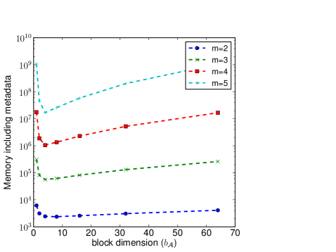
Refer to caption Refer to caption
Fig. 14: Left: Storage requirements of 𝓐[m,64]𝓐superscript𝑚64\displaystyle\bm{\mathscr{{A}}}\in\mathbb{R}^{[m,64]} as block dimension changes. Right: Storage requirements of 𝓐[5,64]𝓐superscript564\displaystyle\bm{\mathscr{{A}}}\in\mathbb{R}^{[5,64]} for different choices for the meta-data stored per block, measured by k𝑘\displaystyle k, as block dimension changes.

We now give a few details about the particular implementation of BCSS, and how this impacts storage requirements. Notice that this is one choice for implementing this storage scheme in practice. One can envision other options that, at the expense of added complexity in the code, reduce the memory footprint.

BCSS views tensors hierarchically. At the top level, there is a tensor where each element of that tensor is itself a tensor (block). Our way of implementing this stores a description (meta-data) for a block in each element of the top-level tensor. This meta-data adds to memory requirements. In our current implementation, the top-level tensor of meta-data is itself a dense tensor. The meta-data in the upper hypertriangular tensor describes stored blocks. The meta-data in the rest of the top-level tensor reference the blocks that correspond to those in the upper hypertriangular tensor (thus requiring an awareness of the permutation needed to take a stored block and transform it). This design choice greatly simplifies our implementation (which we hope to describe in a future paper). We show that although the meta-data can potentially require considerable space, this can be easily mitigated. We use 𝓐𝓐\displaystyle\bm{\mathscr{{A}}} for example purposes.

Given 𝓐[m,n]𝓐superscript𝑚𝑛\displaystyle\bm{\mathscr{{A}}}\in\mathbb{R}^{[m,n]} stored with BCSS with block dimension b𝓐subscript𝑏𝓐\displaystyle b_{\bm{\mathscr{{A}}}}, we must store meta-data for n¯msuperscript¯𝑛𝑚\displaystyle\bar{n}^{m} blocks where n¯=n/b𝓐¯𝑛𝑛subscript𝑏𝓐\displaystyle\bar{n}=\lceil n/b_{\bm{\mathscr{{A}}}}\rceil. This means that the total cost of storing 𝓐𝓐\displaystyle\bm{\mathscr{{A}}} with BCSS is

Cstorage(𝓐)=kn¯m+b𝓐m(n¯+m1m) floats,subscript𝐶storage𝓐𝑘superscript¯𝑛𝑚superscriptsubscript𝑏𝓐𝑚binomial¯𝑛𝑚1𝑚 floats\displaystyle C_{\rm storage}(\bm{\mathscr{{A}}})=k\bar{n}^{m}+b_{\bm{\mathscr{{A}}}}^{m}\binom{\bar{n}+m-1}{m}\mbox{~{}floats},

k𝑘\displaystyle k is a constant representing the amount of storage required for the meta-data associated with one block, in floats. Obviously, this meta-data is of a different datatype, but floats will be our unit.

There is a tradeoff between the cost for storing the meta-data and the actually entries of 𝓐𝓐\displaystyle\bm{\mathscr{{A}}}, parameterized by the blocksize b𝓐subscript𝑏𝓐\displaystyle b_{\bm{\mathscr{{A}}}}:

  • If b𝓐=nsubscript𝑏𝓐𝑛\displaystyle b_{\bm{\mathscr{{A}}}}=n, then we only require a minimal amount of memory for meta-data, k𝑘\displaystyle k floats, but must store all entries of 𝓐𝓐\displaystyle\bm{\mathscr{{A}}} since there now is only one block, and that block uses dense storage. We thus store slightly more than we would if we stored the tensor without symmetry.

  • If b𝓐=1subscript𝑏𝓐1\displaystyle b_{\bm{\mathscr{{A}}}}=1, then n¯=n¯𝑛𝑛\displaystyle\bar{n}=n and we must store meta-data for each element, meaning we store much more data than if we just used a dense storage scheme.

Picking a block dimension somewhere between these two extremes results in a smaller footprint overall. For example, if we choose a block dimension b𝓐=nsubscript𝑏𝓐𝑛\displaystyle b_{\bm{\mathscr{{A}}}}=\sqrt{n}, then n¯=n¯𝑛𝑛\displaystyle\bar{n}=\sqrt{n} and the total storage required to store 𝓐𝓐\displaystyle\bm{\mathscr{{A}}} with BCSS is

Cstorage(𝓐)=kn¯m+b𝓐m(n¯+m1m)=knm2+nm2(nm2+m1m)knm2+nm2(nm2m!)=nm2(k+nm2m!) floats,subscript𝐶storage𝓐𝑘superscript¯𝑛𝑚superscriptsubscript𝑏𝓐𝑚binomial¯𝑛𝑚1𝑚𝑘superscript𝑛𝑚2superscript𝑛𝑚2binomialsuperscript𝑛𝑚2𝑚1𝑚missing-subexpression𝑘superscript𝑛𝑚2superscript𝑛𝑚2superscript𝑛𝑚2𝑚superscript𝑛𝑚2𝑘superscript𝑛𝑚2𝑚 floats\displaystyle\begin{array}[]{l c l}C_{\rm storage(\bm{\mathscr{{A}}})}&=&k\bar{n}^{m}+b_{\bm{\mathscr{{A}}}}^{m}\binom{\bar{n}+m-1}{m}=kn^{\frac{m}{2}}+n^{\frac{m}{2}}\binom{n^{\frac{m}{2}}+m-1}{m}\\ &\approx&kn^{\frac{m}{2}}+n^{\frac{m}{2}}\left(\frac{n^{\frac{m}{2}}}{m!}\right)=n^{\frac{m}{2}}\left(k+\frac{n^{\frac{m}{2}}}{m!}\right)\mbox{~{}\rm floats},\\ \end{array}

which, provided that knm22much-less-than𝑘superscript𝑛𝑚22\displaystyle k\ll\frac{n^{\frac{m}{2}}}{2}, is significantly smaller than the storage required for the dense case (nmsuperscript𝑛𝑚\displaystyle n^{m}). This discussion suggests that a point exists that requires less storage than the dense case (showing that BCSS is a feasible solution).

In Figure 14, we illustrate that as long as we pick a block dimension that is greater than 44\displaystyle 4, we avoid incurring extra costs due to meta-data storage. It should be noted that changing the dimension of the tensors also has no effect on the minimum, however if they are too small, then the dense storage scheme may be the minimal storage scheme. Additionally, adjusting the order of tensors has no real effect on the block dimension associated with minimal storage. However increasing the amount of storage allotted for meta-data slowly shifts the optimal block dimension choice towards the dense storage case.