Properties of the Nonparametric Maximum Likelihood ROC Model with a Monotonic Likelihood Ratio

Abstract

We expect that some observers in perceptual signal detection experiments, such as radiologists, will make rational decisions, and therefore ratings from those observers are expected to form a convex ROC curve. However, measured and published curves are often not convex. This article examines the convexity-constrained nonparametric maximum likelihood estimator of the ROC curve given by Lloyd (2002). Like Lloyd we use the Pool Adjacent Violator Algorithm (PAVA) to construct the estimate of the convex curve. We present a direct proof that this estimate is a convex hull of the empirical ROC curve. The estimate is simple to construct by hand, and follows the suggestions by Pesce, et al. (2010).

We examine the properties of this constrained nonparametric maximum likelihood estimator (NPMLE) under a large number of experimental conditions. In particular we examine the behavior of the area under the curve which is often used as summary metric of diagnostic performance. This constrained ROC estimator gives an area under the curve (AUC) estimate that is biased high with respect to the usual empirical AUC estimate, but may be less biased with respect to the underlying continuous true AUC value. The constrained ROC estimator has lower variance than the usual empirical one. Unlike previous authors who used complex bootstrapping to estimate the variance of the constrained NPMLE we demonstrate that standard unbiased estimators of variance work well to estimate the variance of the NPMLE AUC.

1 Introduction

In signal detection experiments, such as diagnostic medical imaging studies, an image is presented to an observer who gives an ordered categorical rating or score that indicates his confidence in the presence of a signal or disease in that image. For example, a subject may give a rating of one through five, with five indicating the observer is very confident that the image contains a signal. The probability distribution of ratings given to the subjects who have disease we call $F$, and the distribution of ratings given to the subjects who do not have disease we call $H$. Example densities are shown in Figure 1. Typically we assume that these ratings arise from some continuous underlying perceptual distribution and are discretized by the observer for convenience.

From this task we can create measures of diagnostic performance. At each rating category we can calculate the true postive rate (TPR), also called sensitivity, and the false positive rate (FPR) or 1-specificity. The plot of TPR versus FPR across all ordered categories yields an empirical estimate of the Receiver Operating Characteristic (ROC) curve (Green & Swets, 1966). An example of such a curve is shown in Figure 3. The area under an ROC curve (AUC) is the probability that the radiologist will give a higher rating to a diseased patient than a patient without disease and is used to rate the performance of the diagnoses.

An ROC curve that is not convex implies that a human observer, such as a radiologist, will give high ratings to some of the images with signal or disease, but also give such images very low ratings, even lower than the ratings given to completely images with no signal. The higher ratings are expected, but the lower ratings are irrational. There is no reason in general that a human observer would give the lowest of his ratings to images that really contain a signal. Logically, scientists believe that in the limit of barely perceptible signals the worst that human observers could do is guess, in other words, assign a low rating to a signal present or signal absent image with equal probability. Theoretically the likelihood ratio of a pair of distributions, $\text{d}F/\text{d}H$, that model human detection responses should be a monotonically increasing function of the rating given by the observer. Models of ROC data that have monotonic likelihood ratios are called “proper.” (Green & Swets, 1966; Dorfman et al., 1997; Metz & Pan, 1999; Lloyd, 2002) Pesce et al. (2010) detail why we should expect to see convex ROC curves under the assumption that radiologists would perform their task at least as accurately as guessing, and they propose a method for constructing a convex ROC curve estimate.

In this paper we examine the nonparametric maximum likelihood estimate (NPMLE) of the ROC curve under the constraint that its likelihood ratio be monotonic that was first developed by Lloyd (2002). Like Lim & Won (2012) we prove that this estimate is equivalent to a simple convex hull around the usual empirical or unconstrained nonparametric ROC curve MLE. Unlike Lim & Won (2012) we prove this directly from the likelihood and constraints thereon.

This paper examines the properties of the constrained ROC NPMLE under a large number of population parameters. In particular we evaluate the properties of the associated AUC estimate, the area under the the constrained ROC NPMLE. We demonstrate that this estimate has less variance than an unconstrained estimator, and it may have less bias for discretized data.

Unlike Lloyd (2002) and Lim & Won (2012), who used numerical bootstrap techniques to estimate the variance of parameters of the constrained ROC curve MLE, we have found that standard estimators of AUC variance may be used to obtain variance estimates of constrained nonparametric maximum likelihood AUC estimate. Over a wide range of simulation configurations we have found that these estimates are nearly unbiased and very robust. In summary this constrained estimator has a rational convex ROC curve, is simple to construct, it may have small bias, its variance is easily estimated, and therefore it may be useful in observer performance experiments.

2 Data

2.1 Notation

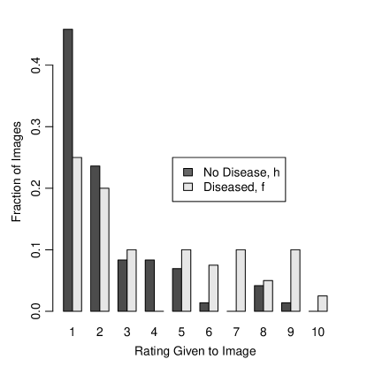
Figure 1: This figure shows two discrete density functions of ordinal observations from two different classes of objects, images with disease and images with no disease. This data is from Chan et al. (2001) and is also given in Table 4. The empirical cumulative distributions of these data sets can be plotted against each other to form the ROC curve shown in Figure 3.

Our data of interest is typically ordered categorical data collected from humans observing two classes of objects.

Let

$x_{1},\dots,x_{N}$ be an IID random sample of ratings or scores from the signal-absent or non-diseased population with density $h$, let

$y_{1},\ldots,y_{M}$ be a random sample from the signal-present or diseased population with density $f$. All ratings are assumed to be discrete in $k$ ordered categories. Each signal-present score $y_{s},~{}s=1\dots M$ corresponds to a category index $d_{s}$, and each signal-absent score $x_{r},~{}r=1\dots N$ corresponds to a category $c_{r}$. There are $m_{i}$ signal observations and $n_{i}$ signal-absent observations in the $i^{th}$ category. For simplicity we assumed the scores in each signal-absent category $i$ to be all identically equal to $\bar{x}_{i}$ and the scores in each signal-present category $j$ to be all identically equal to $\bar{y}_{j}$.

Let $N=\displaystyle\sum_{i=1}^{k}n_{i}$, and $M=\displaystyle\sum_{i=1}^{k}m_{i}$.

2.2 Example Data Sets

As examples we have selected data sets from a study by Chan et al. (2001). In the study, radiologists reviewed X-ray images of mammographic microcalcifications (lesions) that were digitized at different resolutions. Every radiologist rated each lesion from one to ten at every resolution. Higher ratings indicated a radiologist’s greater confidence in the malignancy of the lesion. Radiologists gave lower ratings to lesions that they believed to be benign. The study measured the ability of radiologists to differentiate malignant lesions from benign lesions as a function of the image resolution as measured by the area under the ROC curve (AUC). In the study the authors used a bi-normal parametric method as in Dorfman & Alf (1969) to estimate the ROC curve from the ten-category data.

The distribution of scores from radiologist 5 evaluating the lesions at a resolution 140 microns is given in Figure 1.

Figure 3a shows the empirical ROC curve derived from this data. Easily visible in the figure are the 10 solid line segments derived from the 10 rating categories. We observe that the empirical ROC curve is not convex for this given data set. Later in Section 7 we use this data and ratings from radiologist 4 at a resolution of 35 microns to demonstrate the methods described in this paper.

In this experiment we have confidence that doctors will not systematically give lower ratings to images that contain lesions, nor will they

systematically give higher ratings to images with no lesions. Therefore we believe the true underlying population ROC curves will be convex, and any nonconvexity in these empirical ROC curve estimates is merely due to statistical uncertainty from finite sample size. The average ROC curve across all radiologists and experiments in Figure 7 of Chan et al. (2001) supports this assertion.

3 Likelihood Function

The usual likelihood (Owen, 2001, 1988) of obtaining the categorized ratings for both signal present and absent observations from our experiments given our estimates of $F$ and $H$ is

$$\mathscr{L}\propto\displaystyle\prod_{i=1}^{k}p_{i}^{m_{i}}q_{i}^{n_{i}}$$ (1)

where $p_{i}=dF(\bar{y}_{i})=F(\bar{y}_{i})-F(\bar{y}_{i}-);q_{i}=dH(\bar{x}_{i})=H(\bar{x}_{i})-H(\bar{x}_{i}-)$, and $\bar{y}_{i}-$ is the largest possible value of $y$ less than $\bar{y}_{i}$. As in the power biased model Qin & Lawless (1994), Vardi (1985), and Vardi (1982), we set $w=p/q$. The likelihood function becomes

$$\mathscr{L}\propto\displaystyle\prod_{i=1}^{k}q_{i}^{n_{i}+m_{i}}w_{i}^{m_{i}}.$$ (2)

We use the Lagrange multipliers as in Anderson (1972) to maximize the likelihood function. Maximizing $\mathscr{L}$ subject to $\displaystyle\sum_{i=1}^{k}q_{i}=1$ and $\displaystyle\sum_{i=1}^{k}q_{i}w_{i}=1$ is equivalent to minimizing

$$-\log(\mathscr{L})=\displaystyle\sum_{i=1}^{k}-(n_{i}+m_{i})\log(q_{i})-m_{i}\log(w_{i})+C$$ (3)

subject to the same constraints, where $C$ is a constant.

By first minimizing $-\log(\mathscr{L})$ as a function of $q_{i}\dots,q_{k}$ we obtain $q_{i}=\frac{m_{i}+n_{i}}{N+Mw_{i}}$. Plugging $\frac{m_{i}+n_{i}}{N+Mw_{i}}\text{ for }q_{i}$ in Equation 3 and ignoring the constant terms we are then led to minimize

$$\ell=\displaystyle\sum_{i=1}^{k}(m_{i}+n_{i})\log(N+Mw_{i})-m_{i}\log(w_{i})$$

as a function of $W=(w_{1}\dots,w_{k})$.

4 Estimates

4.1 Unconstrained Estimates

As a function of $w_{1},\dots,w_{k}$, $\ell$ is minimized for $\bar{w}_{i}=\frac{m_{i}/M}{n_{i}/N}.$ We plug $\bar{w}_{i}$ back to $q_{i}=\frac{m_{i}+n_{i}}{N+Mw_{i}}$ and $p_{i}=q_{i}w_{i}$ to obtain the known empirical likelihood estimates $\bar{q}_{i}=\frac{n_{i}}{N}$ and $\bar{p}_{i}=\frac{m_{i}}{M}$.

In what follows we will refer to $\bar{w}_{i}=\frac{m_{i}/M}{n_{i}/N}$ as the unconstrained maximum likelihood ratio (UMLR). We should point out that these estimates of $\bar{q}_{i}$, $\bar{p}_{i}$, and $\bar{w}_{i}$ give the usual empirical ROC curve (Green & Swets, 1966; Bamber, 1975). The empirical likelihood ratios $w_{i}$ are the slopes of the segments of the lines of the empirical ROC curve, i.e. the slopes of the lines in Figure 3a.

4.2 Constrained Estimates

Believing that the true ROC curve is convex, we are led to minimize $\ell=\displaystyle\sum_{i=1}^{k}(m_{i}+n_{i})\log(N+Mw_{i})-m_{i}\log(w_{i})$ subject to the monotonic likelihood ratio constraint $w_{1}\leq w_{2}\leq\dots\leq w_{k}$. This is equivalent to requiring that the slopes of the segments of the ROC curve be increasing from right to left. Let $\bar{p}_{i}~{}\text{and }\bar{q}_{i}$ be defined as in Section 4.1. Let $P_{0}=Q_{0}=1$, and $P_{i}=\displaystyle\sum_{j=1}^{k-i}\bar{p}_{j},~{}Q_{i}=\displaystyle\sum_{j=1}^{k-i}\bar{q}_{j}$, for $i=1\dots k$.

As a function of $w_{1},\dots,w_{k},$ $\ell$ is a sum of k independent functions $\ell_{1},\dots,\ell_{k}$; where $\ell_{i}=(m_{i}+n_{i})\log(N+Mw_{i})-m_{i}\log(w_{i})$ is a function with a single minimum $\bar{w}_{i}$. As shown in Figure 2, $\ell_{i}$ decreases up to $\bar{w}_{i}$ and increases afterward.

Without loss of generality we consider two consecutive functions $\ell_{1}(w)$ and $\ell_{2}(w)$. In Figure 2 we plot $\ell_{1}\text{ and }\ell_{2}$ as functions of $w_{1}\text{ and }w_{2}$ respectively. The graph in Figure 2a shows the UMLR $\bar{w}_{1}\text{ of }\ell_{1}\text{ less than the UMLR }\bar{w}_{2}\text{ of }\ell_{2}$, leading to a convex ROC curve. On the contrary, in Figure 2b we have $\bar{w}_{1}>\bar{w}_{2}$ leading to a nonconvex ROC.

Let $\bar{w}_{1}>\bar{w}_{2}$ as in Figure 2b. Our goal is to find $(\tilde{w}_{1},\tilde{w}_{2})$ such that $\ell_{1}(\tilde{w}_{1})+\ell_{2}(\tilde{w}_{2})=\min\limits_{w_{1}\leq w_{2}}\ell_{1}(w_{1})+\ell_{2}(w_{2})$. In this case, we need to change the ordering of $w_{1}$ and $w_{2}$ while keeping $\ell_{1}(w_{1})+\ell_{2}(w_{2})$ as small as possible.

Let $A(w_{1},\ell_{1}(w_{1}))\text{ and }B(w_{2},\ell_{2}(w_{2}))$ be two arbitrary points as in Figure 2b such that $w_{1}<w_{2}$. Keeping in mind that $\bar{w}_{1}$ and $\bar{w}_{2}$ are the respective global minima of $\ell_{1}\text{ and }\ell_{2}$ we obtain the following inequalities.

$$\text{ If }w_{1}<\bar{w}_{2} \ell_{1}(\bar{w}_{2})+\ell_{2}(\bar{w}_{2})<\ell_{1}(w_{1})+\ell_{2}(w_{2})$$ then

$$\text{ If }\bar{w}_{1}<w_{2} \ell_{1}(\bar{w}_{1})+\ell_{2}(\bar{w}_{1})<\ell_{1}(w_{1})+\ell_{2}(w_{2})$$ then

If $\bar{w}_{2}<w_{1}<w_{2}<\bar{w}_{1}$, $~{}\ell_{1}$ decreases while $\ell_{2}$ increases on the interval $[\bar{w}_{1},\bar{w}_{2}]$, leading to the following inequalities.

$$\ell_{2}(w_{1})<\ell_{2}(w_{2}) \Rightarrow \ell_{1}(w_{1})+\ell_{2}(w_{1})~{}<~{}\ell_{1}(w_{1})+\ell_{2}(w_{2})$$

and

$$\ell_{1}(w_{2})<\ell_{1}(w_{1}) \Rightarrow \ell_{1}(w_{2})+\ell_{2}(w_{2})~{}<~{}\ell_{1}(w_{1})+\ell_{2}(w_{2}).$$

The above inequalities show that the function $\ell_{1}+\ell_{2}$ is never at its minimum for two distinct values of $w_{1}\text{ and }w_{2}$. We deduce that $(\tilde{w}_{1},\tilde{w}_{2})$ satisfies $\tilde{w}_{1}=\tilde{w}_{2}.$ Setting $w_{1}=w_{2}=w$ we minimize the following expression:

$$\ell_{1}(w)+\ell_{2}(w) = (m_{1}+n_{1})\log(N+Mw)-m_{1}\log(w)+$$

$$(m_{2}+n_{2})\log(N+Mw)-m_{2}\log(w)$$

$$= (m_{1}+m_{2}+n_{1}+n_{2})\log(N+Mw)-$$

$$(m_{1}+m_{2})\log(w).$$

Taking the derivative and setting equal to zero we obtain $\tilde{w}=\tilde{w}_{1}=\tilde{w}_{2}=\frac{(m_{1}+m_{2})N}{(n_{1}+n_{2})M}$. Note that for $w_{1}=w_{2}$ we obtain $\ell^{\ast}(w)=\ell_{1}(w)+\ell_{2}(w)$ whose graph is similar to that of either $\ell_{1}\text{ or }\ell_{2}$ from Figure 2. The above proof and conclusions apply to any two adjacent categories in a ROC curve where the unconstrained likelihood ratios are not increasing.

The above demonstrates analytically that the obtained estimate is the constrained maximum likelihood estimate of the non-parametric model.

Note that the constrained estimators $\tilde{w}=\tilde{w}_{1}=\tilde{w}_{2}$ yield a solution that is equivalent to adding the two adjacent categories in to a single category with counts $\tilde{m}=m_{1}+m_{2}$ and $\tilde{n}=n_{1}+n_{2}$. To find all constrained estimates $\tilde{w}_{i}$ in a sequence of $\ell_{i}$, we use an algorithm similar to Lloyd (2002).

5 PAVA: Pool Adjacent Violator Algorithm

The PAVA, a simple iterative algorithm, is a standard nonparametric method used to produce point estimates for a function known to be monotone (Barlow et al., 1972; Robertson et al., 1988; Best & Chakravarti, 1990).

It replaces each stretch of monotonicity-violating observations with the weighted average of the original function values in that stretch.

In order to apply the theoretical approached described above, we developed an R (R Development Core Team, 2009) version of the PAVA algoritm similar to that of Lloyd (2002). As in Section 2, we assume the data has been discretized into k different categories. Keeping in mind that each signal-present score $y_{s}$ corresponds to a category $d_{s}$ and each signal-absent score $x_{r}$ corresponds to a category $c_{r}$ as assumed in Section 2, as the PAVA combines categories it also reassigns each data score to a new category.

We sequentially describe the PAVA as follows.

1. $\tilde{k}\leftarrow k;~{}$ for all $i$, $\tilde{w}_{i}\leftarrow\bar{w}_{i}=\frac{m_{i}N}{n_{i}M};\tilde{m}_{i}\leftarrow m_{i};\tilde{n}_{i}\leftarrow n_{i}$; for all $s$, and for all $r$, $\tilde{d}_{s}\leftarrow d_{s};~{}\tilde{c}_{r}\leftarrow c_{r}$

2. Stop if ROC curve is convex; meaning, $\tilde{w}_{1}\leq...\leq\tilde{w}_{\tilde{k}}$. Otherwise there exists $i$ in $1:\tilde{k}-1$ such that $\tilde{w}_{i}>\tilde{w}_{i+1}.$ If so, continue.

3. The two categories $i$ and $i+1$ are combined into category $i$. $\tilde{m}_{i}\leftarrow\tilde{m}_{i}+\tilde{m}_{i+1},~{}\tilde{n}_{i}\leftarrow\tilde{n}_{i}+\tilde{n}_{i+1};\tilde{w}_{i}\leftarrow\frac{\tilde{m}_{i}N}{\tilde{n}_{i}M}$.

4. After combining the two categories $i$ and $i+1$ into category $i$, the following commands describe how we eliminate category $i+1$, reorganize the remaining categories, and reassign the score category indexes .
   For $s=1\dots M,\text{ if }\tilde{d}_{s}>i\,\text{ then }\tilde{d}_{s}\leftarrow\tilde{d}_{s}-1;$
   for $r=1\dots N,\text{ if }\tilde{c}_{r}>i\text{ then }\tilde{c}_{r}\leftarrow\tilde{c}_{r}-1;$
   for $j=i+1\dots\tilde{k}-1,~{}\tilde{n}_{j}\leftarrow\tilde{n}_{j+1};~{}\tilde{m}_{j}\leftarrow\tilde{m}_{j+1};~{}\tilde{w}_{j}\leftarrow\tilde{w}_{j+1}$;
   $\tilde{k}\leftarrow\tilde{k}-1.$

5. Go to step 2. Proceed until ROC curve is convex.

Applied to the data, the PAVA creates a new data set with total number of categories $\tilde{k}$ which is less than or equal to $k$. We respectively denote the number of signal-absent scores in each new i-category, the number of signal-present scores in each new i-category, the new signal-present category index, and the new signal-absent category index of the new data set by $\tilde{n}_{i}$, $\tilde{m}_{i}$, $\tilde{d}_{s}$, and $\tilde{c}_{r}$.

The dashed line in Figure 3b is obtained from applying the PAVA to the ROC curve in Figure 3a. In Figure 3a we have k=10. Let $p_{i},~{}q_{i},~{}P_{i}\text{ and}~{}Q_{i}$ be defined as in Section 4.2. In the first step there is a violation for $i=3$, i.e $\bar{w}_{3}$ is greater than $\bar{w}_{4}$. The two segments $S_{3}\text{ and }S_{4}$ are replaced by a single segment $S^{\prime}_{3}$ from $(Q_{2},P_{2})\text{ to }(Q_{4},P_{4})$ and $\tilde{w}_{3}$ is set set equal to $(\frac{m_{3}+m_{4}}{M}/\frac{n_{3}+n_{4}}{N})$. This leads to another violation as the new $\tilde{w}_{3}$ is less than $\bar{w}_{2}$. We then replace $S_{2}\text{ and }S^{\prime}_{3}$ by a single segment $S^{\prime}_{2}$ from $(Q_{1},P_{1})\text{ to }(Q_{4},P_{4})\text{ and }\tilde{w}_{2}$ is set equal to $\frac{(m_{2}+m_{3}+m_{4})N}{(n_{2}+n_{3}+n_{4})M}$.

In the next step the PAVA encounters another violation between the segments $S_{6}\text{ and }S_{7}$; the segments $S_{6}\text{ and }S_{7}$ are replaced by a single segment $S^{\prime}_{6}$ . In the final step, the PAVA encounters another violation as the slope of $S^{\prime}_{6}$ is greater than the slope of $S_{8}$; we then replace $S\prime_{6}\text{ and }S_{8}$ by a single segment and the ROC is convex.

An intuitive reason for implementing the algorithm can be summarized as this:

Given that observers will not perform worse than guessing we assume that any non-convexity in a measured empirical ROC curve is due to a statistical variation from insufficient counts in a particular rating category. We therefore combine adjacent ordinal categories until the number of counts in the combined categories are sufficient to generate a plausible convex ROC curve.

This PAVA algorithm is equivalent to the algorithm given in Section 1.2 of Robertson et al. (1988). Specifically using Robertson’s w, $g$, $W$, and $G$ notation let w$(\bar{x}_{i})=\frac{n_{i}}{N},~{}~{}g(\bar{x}_{i})=\frac{m_{i}}{M}/\frac{n_{i}}{N},~{}~{}W_{j}=\displaystyle\sum_{i=1}^{j}\text{w}_{j},~{}G_{j}=\displaystyle\sum_{i=1}^{j}g(\bar{x}_{i})\text{w}(\bar{x}_{i})$. Then the ROC curve, a plot of $P_{j}=(W_{j},G_{j}),~{}j=0,1,\dots,k\text{ with }P_{0}=(0,0)$ is the cumulative sum diagram (CSD) for the function g with weight w. Adapting Robertson’s approach, finding the best convex plot from the nonconvex one reduces to finding the greatest convex minorant (GCM) of the CSD in the interval $[0,Z_{k}]$ for the function g with weight z. This method will lead to the same estimate obtained in Section 4.2.

(a) Likelihoods of a Convex Estimate

(b) Likelihoods of a Non-convex Estimate

Figure 2: These are graphs of the negative log likelihood components $\ell$ as a function of the likelihood ratios $w$.The unconstrained minimum of $\ell_{i}\text{ is }\bar{w}_{i}$. In Figure 2a the unconstrained minimum $\bar{w}_{1}$ of the $-\log$ likelihood function $\ell_{1}$ is less than the unconstrained minimum $\bar{w}_{2}$ of $\ell_{2}$ ; therefore, the likelihood function $\ell=\ell_{1}+\ell_{2}$ yields a convex ROC. In Figure 2b $\bar{w}_{1}>\bar{w}_{2}$ meaning the corresponding -$\log$ likelihood ratio yields a non-convex ROC curve.

(a) NPMLE ROC Curve

(b) Constrained NPMLE ROC Curve

Figure 3: In Figure 3a we plotted the ROC curve of the data from Chan et al. (2001) described in Section 2.2 and given in Table 4. The ROC curve is the set all possible measurable specificity and sensitivity pairs. We obtained the constrained estimate (dotted line) in Figure 3b by applying the PAVA to the data used in Figure 3a. In Figure 3a we have $k=10$ line segments. $P_{i}\text{ and}~{}Q_{i}$ are defined in Section 4.2. Segments $S_{2}$, $S_{3}$, and $S_{4}$ form a violation because the slope $\bar{w}_{4}$ of segment $S_{4}$ is so low. Therefore we replace those 3 segments with a single segment $S^{\prime}_{2}$ with slope $\tilde{w}_{2}={(m_{2}+m_{3}+m_{4})N}/{(n_{2}+n_{3}+n_{4})M}$ Also see Table 4. Categories $S_{6}$, $S_{7}$, and $S_{8}$ also form a violation and are replaced with a single category.

To verify that the above solution really is the maximum likelihood estimate under the constraint of a monotonic likelihood ratio, we wrote a software function whose input is a combined vector of $p_{i}\text{ and }q_{i}$ and whose output is the likelihood function given in Expression 1 if the ROC curve is convex. If the ROC curve is not convex, the output is a value less than zero. We then used a numerical optimizer (“optim” from the package R (R Development Core Team, 2009)) to maximize the function over all inputs $p_{i},q_{i}$ on many random simulated data sets with random initial values. The maximum likelihood function given by the optimizer was usually equal to that obtained from the PAVA. All other times the optimizer failed to converge or converged to a local maximum with likelihood less than that obtained from the PAVA. This verified numerically that the PAVA gives the constrained maximum likelihood.

6 Bias and Variance Estimation of AUC

The Wilcoxon-Mann-Whitney statistic is equivalent to the area under the ROC curve (AUC) and is frequently used as a summary measure of separability of the observations that contain a signal from observations that do not, or separability of images that have disease from those who do not. The area under the population ROC curve is equal to the probability that a rating of an image with a signal is higher than a signal-absent rating, AUC$=P(Y>X)$ (Bamber, 1975). The area under the unconstrained empirical maximum-likelihood ROC curve estimate is

$$\widehat{AUC}=\frac{1}{NM}\sum_{r=1}^{N}\sum_{s=1}^{M}I_{rs}$$ (4)

We assume that each pair (r,s) corresponds to a pair $(c_{r},d_{s})$ such that $x_{r}$ belongs to the category $c_{r}$ and $y_{s}$ belongs to the category $d_{s}$.

$$I_{rs}=\left\{\begin{array}[]{rlll}\frac{1}{2}&\text{ if }c_{r}=d_{s}\\ 0&\text{ if }c_{r}>d_{s}\\ 1&\text{ if }c_{r}<d_{s}\end{array}\right.$$ (5)

The area under the constrained empirical maximum-likelihood ROC curve estimate has the same form and is

$$\widetilde{AUC}=\frac{1}{NM}\sum_{r=1}^{N}\sum_{s=1}^{M}I^{\prime}_{rs}$$ (6)

where

$$I^{\prime}_{rs}=\left\{\begin{array}[]{rlll}\frac{1}{2}&\text{ if }\tilde{c}_{r}=\tilde{d}_{s}\\ 0&\text{ if }\tilde{c}_{r}>\tilde{d}_{s}\\ 1&\text{ if }\tilde{c}_{r}<\tilde{d}_{s}\end{array}\right.$$ (7)

In this Section we use simulated data to measure how the constrained AUC estimate differs from the unconstrained AUC estimate and a true continuous AUC population value. We also examine ways to estimate variance of the constrained AUC estimate.

6.1 Simulation Parameters

We simulated data from normal distributions, D=$\mathcal{N}(\mu,1)$, and from uniform distributions, D=$\mathcal{U}(0,\mathfrak{m})$, which are uniform in probability between 0 and $\mathfrak{m}$. For the uniform distributions $\mathcal{U}$, the non-diseased or signal-absent sample is drawn from $\mathcal{U}(0,1)$, and the signal-present or diseased sample is drawn from $\mathcal{U}(0,\mathfrak{m})$ where $\mathfrak{m}\geq 1$. Both samples together form a combined sample. In order to have the desired $AUC$ value for the uniform distribution, it follows from $AUC=P(Y>X)$ that $AUC=1-\frac{1}{2\mathfrak{m}}$ from which we derive $\mathfrak{m}=\frac{1}{2(1-AUC)}.$ This pair of uniform distributions yields the most asymmetric ROC curve that still has a monotonically increasing likelihood ratio.

For the normal distribution $\mathcal{N}$, the diseased sample is drawn from $N(\mu,1)$ and the non-diseased sample is drawn from $\mathcal{N}(0,1)$. To achieve the desired $AUC$, we used $P(Y>X)=\Phi\left(\frac{\mu_{Y}-\mu_{X}}{\sqrt{\sigma_{X}^{2}+\sigma_{Y}^{2}}}\right)$, where $\Phi$ is the cumulative normal distribution function, $\mu_{Y}=\mu$, and $\mu_{X}=0$. We set $\mu=\sqrt{2}\Phi^{-1}(AUC)$. This model gives a continous symmetric convex ROC curve.

6.2 Bias Study

We first considered a vector of AUC values with elements ranging from .6 to .99 with step equal to .01. For each AUC value from the above vector, we sampled data from either normal distributions, D=$\mathcal{N}$, or uniform distributions, D=$\mathcal{U}$. We simulated 10,000 independent random combined samples from D. Each combined random sample consisted of a sample of size 55 drawn from the non-diseased distribution and a sample of size 110 drawn from the non-diseased population. These sample size are typical in many studies in medical literature. We then discretize each sample into seven categories. For each discretized combined sample we computed the usual unconstrained AUC estimate, then applied the PAVA algorithm and computed the constrained AUC estimate.

In Figure 4 we plotted the average constrained and unconstrained AUC estimates from the normally distributed simulation versus the true AUC. We first note that the average unconstrained AUC estimate is always biased low with respect to the true undiscretized population AUC. This reduction of information and AUC estimates due to discretization is well known. We also note that the average constrained AUC estimate is always greater than the average unconstrained AUC estimate. This result is consistent with the construction of the constrained ROC curve in Section 4.2. To construct the constrained ROC estimate we combine categories in a way that always increases the area under the curve. With respect to the true population AUC, the average constrained AUC estimate is sometimes less, sometimes greater, depending on the value of AUC. Depending on AUC, sample size, and discreteness of data, the constrained estimate may be less biased than the unconstrained estimate.

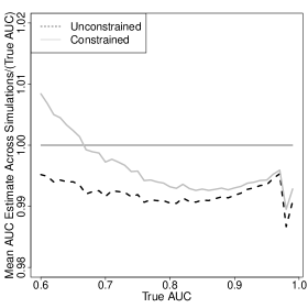
Figure 4: This figure shows the fractional bias (the mean estimated value divided by the true value) of the two nonparametric estimators of AUC in this paper as a function of AUC. The mean of the usual unconstrained nonparametric AUC estimate (equation 4) is always less than the true underlying simulation AUC value because the observed values are discretized. The constrained AUC estimate (equation 6) is always greater than the unconstrained AUC estimate. The constrained AUC estimate can be considered less biased than the usual unconstrained emprirical AUC estimate for most values of the AUC.

6.3 Variance Estimation of the AUC

In this Section we demonstrate empirically that a standard variance estimator of the empirical area under the curve (AUC) also provides a good estimate the AUC of the above convexity-restricted ROC curve estimate. Our method of variance estimation can be considered as a two-way analysis of variance (ANOVA) with one observation per cell as in Chapter 7 of Sheffé (2009). We model $I_{rs}$ where each cell consists of 1 if the diseased score $s$ is greater than the non-diseased score $r$, of $\frac{1}{2}$ if both scores are equal, and 0 otherwise. See equation 5. The model is $I_{rs}=\mu+a_{r}+b_{s}+\epsilon_{rs}$ for $r=1...N$;$s=1\dots M$, or equivalently for AUC, $\hat{A}=\frac{1}{NM}\displaystyle\sum\limits_{r=1}^{N}\sum\limits_{s=1}^{M}(\mu+a_{r}+b_{s}+\varepsilon_{rs})$ where $\mu$ represents the overall mean AUC. The random variable $a_{r}$ has mean zero and variance $\sigma_{a}$ reflecting the variability between the disease tests. $b_{s}$ has mean 0 and variance $\sigma_{b}$ reflecting the variability between the non-disease tests. $\varepsilon_{rs}$ has mean zero and variance $\sigma_{\varepsilon}$ representing the interaction between disease and non-disease tests. The total variance of $\hat{A}$ is

$$\text{Var}(\hat{A})=\frac{\sigma^{2}_{a}}{N}+\frac{\sigma^{b}_{b}}{M}+\frac{\sigma^{2}_{\varepsilon}}{NM}$$ (8)

The respective estimates $\hat{\sigma}_{a},~{}\hat{\sigma}_{b},\text{ and }\hat{\sigma}_{\varepsilon}$ of $\sigma_{a},~{}\sigma_{b},\text{ and }\sigma_{\varepsilon}$ are computed as in equation 7.4.10 of Sheffé (2009). For simulation purposes, we chose the distribution D=$\mathcal{U}$ or D=$\mathcal{N}$ as in Section 6.2 and then chose the parameters of the distribution so that AUC=.6, AUC= .84, and AUC=.94 which respectively correspond to $\mathfrak{m}=1.25,\mathfrak{m}=3.125,\text{ and }\mathfrak{m}=25/3$ for D=$\mathcal{U}$ and to $\mu=.358,~{}\mu=1.406,~{}\text{ and }\mu=2.199$ for D=$\mathcal{N}$. There are often more non-disease patients available than disease patients. With that in mind, we assumed in the simulation the ratio of non-disease sample size to diseased sample size to take values $r_{a}=1,r_{a}=3$, and $r_{a}=9$. This means for each combined sample set consists of $M$ observations treated as diseased and $N=r_{a}\times M$ treated as non-diseased. We discretized each sample into k categories, where k takes values k=3, k=7, and k=16. For each quadruple $(D,M,r_{a},k)$, we generated 10,000 independent sets of combined random samples from the chosen distribution.

For each quadruple $(D,M,r_{a},k)$, we computed the unconstrained AUC $\hat{A}_{u}^{j}$ and the estimate of variance $\widehat{V}_{u}^{j}$ using Expression 8. We then applied the PAVA algorithm, computed the constrained AUC $\widehat{A}_{c}^{j}$, computed the estimate of the constrained AUC variance $\widehat{V}_{c}^{j}$ using Expression 8. We then computed an approximate confidence interval of the AUC, $I^{cj}_{1-\alpha}=\left[\widehat{A}_{c}^{j}-z_{\alpha/2}\sqrt{\widehat{V}_{c}^{j}},\widehat{A}_{c}^{j}+z_{\alpha/2}\sqrt{\widehat{V}_{c}^{j}}\right],\text{ for }\alpha=.05$, where $z_{\alpha}$ is the standard normal deviate with probability $\alpha$.

For each combined sample set of $10^{4}$ simulations, we plotted the square root of the mean of all the unconstrained variance estimates $\widehat{V}_{u}^{j}$ versus the standard deviation across all the simulated unconstrained AUC $\widehat{A}_{u}^{j}$ in Figure 5. These data points lie on the diagonal of the plot indicating that our estimate of the variance of the empirical AUC estimate is unbiased (Gallas & et al., 2009).

Also in Figure 5 we plotted the square root of the mean of the constrained variance estimates $\widehat{V}_{c}^{j}$ versus the standard deviation across all the simulated constrained AUC $\widehat{A}_{c}^{j}$. We note from these plots that the true standard deviation of AUC of the constrained ROC curves are lower on average than the standard deviation of the AUC of the unconstrained ROC curves, and the mean estimate of the standard deviation is reduced by almost exactly the same amount.

From the figure it is apparent that our standard estimator of empirical AUC variance also very well estimates the variance of the constrained empirical estimate of AUC, and it is robust against the large range of parameters over which we varied the simulation.

To test this assertion we report in Table 2 the coverage probabilities, which are the fractions of the simulations falling outside the above estimated confidence interval $I^{cj}_{1-\alpha}$. From Table 2 we observe that the overall performance of the estimate of variance is accurate except in a few cases where the following conditions exist simultaneously: a large AUC, small sample size and a large number of categories.

Note that there is nothing special about the AUC variance estimator that we used. Other variance estimates (Bamber, 1975; Campbell, 1994) also make useful measures the variance of the constrained AUC estimate. These simple analytic variance estimators agree well with bootstrap estimation techniques (Efron & Tibshirani, 1993; Lloyd, 2002; Lim & Won, 2012). This includes the simple AUC variance approximation $\widehat{\text{AUC}}(1-\widehat{\text{AUC}})(N^{-1}+M^{-1})/4$ (Wagner & et al., 1997). This form makes clear the binomial-like behavior of AUC and the expected reduction in variance corresponding to the increase in AUC.

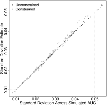
Figure 5: This figure plots the square root of the mean of the variance estimates of AUC as a function of the standard deviations of the AUC estimates of our simulations. Data for both the usual unconstrained empirical AUC estimate and the constrained AUC estimate are displayed. Each point represents $10^{4}$ simulated samples from one of our simulation configurations. The true standard deviation of AUC of the constrained ROC curves are lower on average than the standard deviation of the AUC of the unconstrained ROC curves, and the mean estimate of standard deviation is reduced by almost exactly the same amount.

Table 1: Coverage Intervals with Nominal Level 0.95

UNIFORM DISTRIBUTION
AUC			3 categories				7 categories				16 categories
	ratio $r_{a}$		1	3	9		1	3	9		1	3	9
		M=55	.0526	.0529	.0554		.0710	.0671	.0577		.0632	.0623	.0587
.6		M=100	.0493	.0509	.0536		.0676	.0625	.0583		.0577	.0542	.0578
		M=200	.0627	.0572	.0562		.0593	.0547	.0558		.0534	.0508	.0553
		M=55	.0639	.0644	.0657		.0665	.0697	.0681		.0754	.0736	.0796
.84		M=100	.0597	.0540	.0581		.0564	.0597	.0612		.0644	.0625	.0605
		M=200	.0493	.0537	.0574		.0566	.0569	.0595		.0552	.0574	.0580
		M=55	.0678	.0717	.0696		.0967	.1006	.1048		.1056	.1158	.1206
.94		M=100	.0623	.0659	.0649		.0762	.0808	.0872		.0902	.0901	.0954
		M=200	.0559	.0569	.0557		.0650	.0636	.0639		.0718	.0672	.0684
NORMAL DISTRIBUTION
		M=55	.0519	.0527	.0564		.0628	.0576	.0575		.0597	.0554	.0574
.6		M=100	.0522	.0568	.0523		.0550	.0528	.0497		.0531	.0483	.0490
		N=200	.0489	.0519	.0502		.0532	.0507	.0519		.0520	.0474	.0468
		M=55	.0586	.0585	.0627		.0613	.0598	.0642		.0722	.0643	.0663
.84		M=100	.0514	.0603	.0560		.0596	.0571	.0585		.0602	.0564	.0522
		M=200	.0548	.0548	.0513		.0557	.0509	.0569		.0610	.0564	.0537
		M=55	.0725	.0780	.0830		.0862	.0764	.0765		.0955	.0846	.0891
.94		M=100	.0610	.0648	.0702		.0729	.0623	.0697		.0720	.0716	.0743
		M=200	.0592	.0566	.0623		.0593	.0611	.0645		.0624	.0569	.0614

Table 2: *

We generated 10,000 independent sets of combined random samples. Each combined sample consists of a sample size of $N$ treated as diseased and a sample size of $N=r_{a}\times M$ treated as non-diseased. We discretized each sample into k categories, where k takes values k=3, k=7, and k=16. The coverage probabilities reported in the above table are the fractions of the simulations falling outside the confidence interval $I^{cj}_{1-\alpha}$ described in Section 6. Here $\alpha=0.05$.

7 Application

In Section 5 we showed how to obtain the constrained ROC curve estimate using data from Chan et al. (2001). Figure 3a shows the application of the PAVA to the ROC curve of radiologist 5 described in Section 2.2. Ten ordinal categories were reduced to 6 categories to construct a convex ROC curve. In this section we use the same data to compute the constrained and unconstrained estimates of AUC as well as the estimates of variance of those AUC values. All these estimates are given in Table 5. Also given are the results for radiologist 4 reading images at a different resolution.

Table 3: Distribution of Score Ratings

Ordered Rating Category	1	2	3	4	5	6	7	8	9	10
Diseased Counts ($n_{i}$)	10	8	4	0	4	3	4	2	4	1
Nondiseased Counts ($m_{i}$)	33	17	6	6	5	1	0	3	1	0
Likelihood Ratio ($\bar{w}_{i}$)	0.30	0.47	0.67	0.00	0.80	3.00	$\infty$	0.67	4.00	$\infty$
Constrained Diseased Counts ($\tilde{n_{i}}$)	10	12			4	9			4	1
Constrained Nondiseased Counts ($\tilde{m_{i}}$)	33	29			5	4			1	0
Likelihood Ratio ($\tilde{w_{i}}$)	0.30	0.41			0.80	2.25			4.00	$\infty$

Table 4: *

This table gives the distribution of scores given by radiologist 5 for diseased and nondiseased patients. The lower rows show how adjacent ordered rating categories are combined to obtain a monotonically increasing likelihood ratio. This combined data is then used to construct an ROC curve and estimate AUC and its variance in the same manner as the original data.

	Unconstrained			Constrained
	AUC	Variance		AUC	Variance
Radiologist 4	.7386	.002605		.7618	.002471
Radiologist 5	.6622	.002886		.68472	.002782

Table 5: This table gives the constrained and unconstrained estimates of AUC and the variance AUC given given the ratings of radiologist 5 evaluating lesions at a resolution of 140 microns. The same estimates are given for radiologist number 4 evaluating the lesions at a resolution of 35 microns. The estimates of AUC were calculated using Expressions 4 and 6, and the variance was estimated using Expression 8.

As expected the constrained AUC estimates are greater than the unconstrained AUC estimates. Correspondingly the variance estimates of the constrained AUC estimates are smaller than the unconstrained variance estimates.

8 Summary

In some studies of observer signal-detection performance we may assume that decisions made by human observers are rational, implying the convexity of a population ROC curve. In that scenario we may want to analyze the data under that assumption.

In this paper we examined one such method, the constrained nonparametric maximum likelihood ROC curve estimate given by Lloyd (2002). We proved directly that this this estimate is a simple convex hull around the usual empirical ROC curve. We examined the properties of the area under this estimate and found that it has lower variance than the usual empirical AUC estimate, and it may also have lower bias with respect to a continous nondiscretized ROC curve. Our simulations indicate that standard estimators of variance of the Mann-Whitney-Wilcoxon statistic (AUC) variance may be used to obtain nearly unbiased and very robust variance estimates of constrained nonparametric maximum likelihood AUC estimate. Bootstrapping of the convexity algorithm (PAVA) is not required.

The constrained ROC curve estimate is simple to construct in a manner similar to that suggested in Pesce et al. (2010). First a regular empirical ROC curve is constructed. Then the lowest convex envelope that will enclose this ROC curve is drawn. This envelope is the new constrained nonparametric maximum likelihood ROC curve estimate. Holding the total number of observations constant, we recalculate the number of observations in each category implied by the constrained estimate. This is equivalent to combining adjacent categories that do not have increasing likelihood ratios, as in Table 4. Next we use these new combined observation numbers to calculate the empirical AUC estimate in the usual manner. This is the constrained NPMLE of AUC. We also can use those new combined observations in standard nonparametric estimators of AUC variance to estimate the variance of the constrained NPMLE of AUC. This estimator is a useful option for nonparametric analysis of data from studies of observer signal-detection performance where the observers are assumed to generate convex ROC curves rationally.

9 Acknowledgements

The authors are grateful to Dr. Chan and the other authors of Chan et al. 2001 for the use of their data in this paper.

References

- Anderson (1972) Anderson, J. A. (1972). Separate sample logistic discrimination. Biometrika, 59, 19–35.
- Bamber (1975) Bamber, D. (1975). The area above the ordinal dominance graph and the area below the receiver operating characteristic graph. Journal of mathematical psychology, 12, 387–415.
- Barlow et al. (1972) Barlow, R. E., Bartholomew, D. J., Bremner, J. M., & Brunk, H. D. (1972). Statistical Inference Under Order Restrictions: The Theory and Application of Isotonic Regression. New York: John Wiley & Sons.
- Best & Chakravarti (1990) Best, M. J., & Chakravarti, N. (1990). Active set algorithms for isotonic regression; a unifying framework. Mathematical Programming, 47, 425–439.
- Campbell (1994) Campbell, G. (1994). Advances in statistical methodology for the evaluation of diagnostic and laboratory tests. Statistics in Medicine, 13, 499–508.
- Chan et al. (2001) Chan, H. P., Helvie, M. A., Petrick, N., Sahiner, B., Adler, D. D., Paramagul, C., Roubidoux, M. A., Blane, C. E., Joynt, L. K., Wilson, T. E., Hadjiiski, L. M., & Goodsitt, M. M. (2001). Digital mammography: Observer performance study of the effects of pixel size on the characterization of malignant and benign microcalcifications. Academic Radiololgy, 8, 454–466.
- Dorfman & Alf (1969) Dorfman, D. D., & Alf, E. (1969). Maximum likelihood estimation of parameters of signal detection theory and determination of confidence intervals– rating method data. Journal of Mathematical Psychology, 6, 487.
- Dorfman et al. (1997) Dorfman, D. D., Berbaum, K. S., Metz, C. E., Lenth, R. V., Hanley, J. A., & Dagga, H. A. (1997). Proper receiver operating characteristic analysis: The bigamma model. Academic Radiology, 4, 138–149.
- Efron & Tibshirani (1993) Efron, B., & Tibshirani, R. J. (1993). Introduction to the Bootstrap. Boca Raton: Chapman & Hall/CRC.
- Gallas & et al. (2009) Gallas, B. D., & et al. (2009). A framework for random-effects ROC analysis: Biases with the bootstrap and other variance estimators. Comm. in Stat. - Theory and Methods, 38, 2586–2603.
- Green & Swets (1966) Green, D. M., & Swets, J. A. (1966). Signal Detection Theory and Psychophysics. New York: John Wiley & Sons.
- Lim & Won (2012) Lim, J., & Won, J. (2012). Roc convex hull and nonparametric maximum likelihood estimation. Mach. Learn, 88.
- Lloyd (2002) Lloyd, C. J. (2002). Estimation of a convex ROC curve. Statistics and Probability Letters, 59, 99–111.
- Metz & Pan (1999) Metz, C. E., & Pan, X. (1999). Proper binormal ROC curves: theory and maximum-likelihood estimation. Journal of Mathematical Psychology, 43, 1–33.
- Owen (1988) Owen, A. B. (1988). Empirical likelihood ratio confidence intervals for a single functional. Biomaker, 75, 237–249.
- Owen (2001) Owen, A. B. (2001). Empirical Likelihood: Monographs on Statistics and Applied Probability 82. Boca Raton: CRC.
- Pesce et al. (2010) Pesce, L. L., Metz, C. E., & Berbaum, K. S. (2010). On the convexity of ROC curves estimated from radiological test results. Acad. Rad., 17, 960–968.
- Qin & Lawless (1994) Qin, J., & Lawless, J. (1994). Empirical likelihood and general estimating equations. Ann. Statist., 22, 300–325.
- R Development Core Team (2009) R Development Core Team (2009). R: A Language and Environment for Statistical Computing. R Foundation for Statistical Computing Vienna, Austria. ISBN 3-900051-07-0.
- Robertson et al. (1988) Robertson, T., Wright, F. T., & Dykstra, L. L. (1988). Order Restricted Statistics Inference. New York: Wiley Sons.
- Sheffé (2009) Sheffé, H. (2009). The Analysis of Variance. New Jersey: John Wiley Sons.
- Vardi (1982) Vardi, Y. (1982). Nonparametric estimation in presence of length bias. Ann. Statist., 10, 616–620.
- Vardi (1985) Vardi, Y. (1985). Empirical distributions in selection bias models. Ann. Statist., 13, 178–203.
- Wagner & et al. (1997) Wagner, R. F., & et al. (1997). Finite-sample effects and resampling plans: Applications to linear classifiers in computer-aided diagnosis. In Proc. of the SPIE (pp. 467–477). volume 3034.