Transport through two interacting resonant levels connected by a Fermi sea

Abstract

We study transport at finite bias, i.e. beyond the linear regime, through two interacting resonant levels connected by a Fermi sea, by means of time-dependent density matrix renormalization group. We first consider methodological issues, like the protocol that leads to a current-currying state and the characterization of the steady state. At finite sizes both the current and the occupations of the interacting levels oscillate as a function of time. We determine the amplitude and period of such oscillations as a function of bias. We find that the occupations on the two dots oscillate with a relative phase which depends on the distance between the impurities and on the Fermi momentum of the Fermi sea, as expected for RKKY interactions. Also the approximant to the steady-state current displays oscillations as a function of the distance between the impurities. Such a behavior can be explained by resonances in the free case. We then discuss the incidence of interaction on such a behavior. We conclude by showing the effect of the bias on the current, making connection with the one-impurity case.

I Introduction

The study of quantum transport across nanostructures has been the subject of intense theoretical and experimental attention for decades. One of the most intensively studied systems is that of quantum dots, both because of their great experimental versatility and because they unveil an extremely rich physics, as exemplified by the Kondo effect Hewson (1993) in quantum dots Goldhaber-Gordon et al. (1998); van der Wiel et al. (2000). When considering a system of two quantum dots, a further interesting phenomenon emerges, the Rudermann-Kittel-Kasuya-Yosida (RKKY) interaction Ruderman and Kittel (1954); *Kasuya_PTP56; *Yosida_PR57; *VanVleck_RMP62; *Kittel. It describes the indirect interaction between two magnetic impurities mediated by the electrons of the surrounding Fermi sea, and is characterized by oscillations related to the Fermi wavevector. The competition between the RKKY interaction and the Kondo effect was studied in the frame of numerical renormalization group Jones and Varma (1987); *Jones_PRL88; *Jones_PRB89, and conformal field theory Affleck and Ludwig (1992); Affleck et al. (1995). An experimental realization with two quantum dots coupled by a Fermi sea was meanwhile reported Craig et al. (2004).

Recently, a great deal of progress was achieved towards the theoretical determination of steady-state transport properties focusing on a quantum dot described by the interacting resonant level model (IRLM) Boulat et al. (2008); Karrasch et al. (2010a, b); Kennes and Meden (2012, 2013); Kennes et al. (2012); Andergassen et al. (2011); Schmitteckert (2004a); Branschädel et al. (2010a); Einhellinger et al. (2012), that consists of spinless fermions with a nearest-neighbor repulsive interaction for the sites adjacent to the dot. This model was studied with several theoretical techniques, ranging from integrable field theories and Bethe Ansatz (see Boulat et al. Boulat et al. (2008) and references therein), functional renormalization group Karrasch et al. (2010a, b); Kennes and Meden (2012, 2013); Kennes et al. (2012), real-time renormalization group Andergassen et al. (2011), to density-matrix renormalization group (DMRG) techniques Schmitteckert (2004a); Boulat et al. (2008); Branschädel et al. (2010a); Einhellinger et al. (2012). These works provide the I-V characteristics out of equilibrium at finite bias and up to large values of the interaction Boulat et al. (2008), and a detailed knowledge of the relaxation dynamics Karrasch et al. (2010a, b); Andergassen et al. (2011); Kennes and Meden (2012); Kennes et al. (2012) in the regime of small interaction, including also the incidence of finite temperatures Kennes and Meden (2013). The shot noise and the full counting statistics have been studied by means of exact diagonalization Branschädel et al. (2010b) (in the free case), DMRG and thermodynamical Bethe Ansatz Branschädel et al. (2010c); Carr et al. (2011). Such an attention on a model that arguably cannot be experimentally realized in an electronic system is due to the fact that, in contrast to the Anderson impurity model, the important energy scales of the problem are accessible and controllable in numerical simulations, avoiding to deal with the Kondo scale, that requires high resolution in energy.

In contrast to the great attention devoted to the one impurity case, little is known about the case with more impurities Schneider and Schmitteckert (2006); Enss et al. (2005); Costamagna and Riera (2008); R.A. Molina et al. (2005); Weinmann et al. (2008). In particular, to the best of our knowledge, the case of two IRLs separated by a Fermi sea under a finite bias awaits still a theoretical treatment. Here we consider two leads modeled as tight-binding chains with uniform hopping, coupled to two quantum dots interacting with their nearest-neighboring sites and a Fermi sea in between, focusing on the dynamics of the system when it is taken out of equilibrium with the application of a finite bias. The set-up is that of a quantum quench, where the initial state corresponds to the ground state of a Hamiltonian, but the time evolution is governed by a different (time independent) one. We considered two different protocols, where the bias is included either in the initial or in the final Hamiltonian. We discuss also the characterization of the steady-state and the incidence of finite-size effects.

We performed our studies by means of a time-dependent DMRG (t-DMRG) simulation White and Feiguin (2004); Daley et al. (2004); Schmitteckert (2004b); Schollwöck (2011). This method allows to study the time evolution of the system up to intermediate times ($\sim 40\hbar/t_{0}$, where $t_{0}$ is the nearest-neighbor hopping between the sites of the leads) in a nonperturbative way. The time evolution of the current on each link of the chain and of the particle-density on the dots exhibits oscillations whose frequency depends on the applied bias, as in the single dot case. In the present case the occupations on the two dots oscillate with a relative phase which depends on the distance between the impurities, both in the free and in the interacting case. This can be explained in terms of the RKKY interaction. The currents through the sites connecting the quantum dots to the leads show also oscillations but with a phase-shift with respect to the density. These oscillations are a finite-size effect, as already discussed in the single dot case Branschädel et al. (2010a), and vanish in the limit of infintiely long leads, as shown below. For the approximant to the steady-state current we find that it oscillates as a function of the distance between the impurities. In the free case the behavior of the current can be understood in terms of resonances that appear in the transmission coefficient of a single particle propagating through the system. We then show the effect of interaction. While it suppresses the resonances found in the free case, for strong interaction we find that large oscillations of the current as a function of the interimpurity distance arise. Finally we consider the I-V characteristics in the presence of two impurities, showing also in this context the presence of negative conductance.

This paper is organized as follows. Section II is devoted to the discussion of methodological issues. In particular in Sec. II.1 we define the model, the observables and the numerical technique. We show the effect of different quench schemes and motivate our choice in Sec. II.2. In Sec. II.3 we detail how the approximant of the steady-state current is obtained and benchmark our DMRG results for the one impurity system with those of Boulat et al. Boulat et al. (2008). Section III displays our results. In Sec. III.1 the time evolution of the occupations and the currents is shown and its relation with RKKY interaction is discussed. In Sec. III.2 we concentrate on the approximant to the steady-state values of the current as a function of the distance. We consider first the free case, for which we establish a connection with the problem of transmission of a single particle propagating in the system, and then move to the interacting case. In Sec. III.3 we discuss the I-V characteristics in the presence of interaction, comparing it with the one-impurity case Boulat et al. (2008). In Sec. IV we summarize our results.

II Models and methods

II.1 Hamiltonian and observables

We study a system characterized by the presence of two quantum dots at positions $d_{1}$ and $d_{2}$ separated by a distance $R\equiv d_{2}-d_{1}$. The region inbetween harbours a Fermi sea. The Hamiltonian of the whole system is given by

$${\hat{H}}_{\rm chain}\equiv\hat{H}_{\rm D}+\hat{H}_{\rm T}+\hat{H}_{\rm F}\;,$$ (1)

where

$$\hat{H}_{\rm D} = -t_{{\rm C}}(\hat{c}^{\dagger}_{d_{1}-1}\hat{c}_{d_{1}}+\hat{c}^{\dagger}_{d_{2}}\hat{c}_{d_{2}+1}+{\rm H.c.})$$ (2)

$$-t_{{\rm C}}(\hat{c}^{\dagger}_{d_{1}}\hat{c}_{d_{1}+1}+\hat{c}^{\dagger}_{d_{2}-1}\hat{c}_{d_{2}}+{\rm H.c.})$$

$$+U_{\rm C}\sum_{\alpha=d_{1},d_{2}}\sum_{r=\pm 1}\left(\hat{n}_{\alpha}-\frac{1}{2}\right)\left(\hat{n}_{\alpha+r}-\frac{1}{2}\right)\;,$$

corresponds to the dots and their nearest-neighbors, where the interaction is present. The leads connecting to the quantum dot are described by the tight-binding Hamiltonian $H_{\rm T}$,

$$\hat{H}_{\rm T}=-t_{0}\sum_{j=1}^{d_{1}-2}\hat{c}^{\dagger}_{j}\hat{c}_{j+1}-t_{0}\sum_{j=d_{2}+1}^{L-1}\hat{c}^{\dagger}_{j}\hat{c}_{j+1}+{\rm H.c.}\;.$$ (3)

Furthermore, the Fermi sea is described by the Hamiltonian $H_{\rm F}$,

$$\hat{H}_{\rm F}=-t_{0}\sum_{j=d_{1}+1}^{d_{2}-2}(\hat{c}^{\dagger}_{j}\hat{c}_{j+1}+{\rm H.c.})$$ (4)

In what follows we call the sites at positions $c_{1}\equiv d_{1}-1$ and $c_{2}\equiv d_{2}+1$ contacts. The total number of sites of the system is given by $L$, which we take even. If $R$ is odd, we choose the position of the dots such that the left and the right leads have the same number of sites. If $R$ is even the position of the dots is given by $(L-R)/2+1$ and $(L+R)/2+1$, implying that the left lead has one more site with respect to the right one. In Eqs. (2) - (4) we have $\hat{n}_{j}=\hat{c}^{\dagger}_{j}\hat{c}_{j}$, where $\hat{c}^{\dagger}_{j}$ ($\hat{c}_{j}$) are creation (annihilation) operators for spinless fermions, $U_{{\rm C}}$ is the interaction coupling the dots and their nearest neighbors, $t_{\rm C}$ is the hopping between the dot and its nearest-neighbors. The hopping elements in the leads and in the Fermi sea are all set to $t_{0}$. Energies are measured in units of $t_{0}$ and time in units of $\hbar/t_{0}$. The number of particles in the system is $N$ and we define the average density of particles as $\rho\equiv N/L$. When not explicitly specified, we assume the system at half-filling. We also define $L_{\rm c}\equiv R-1$, $N_{\rm c}$ and $\rho_{\rm c}\equiv N_{\rm c}/L_{\rm c}$ as the number of sites, the number of particles and the density in the central region (from site $d_{1}+1$ to $d_{2}-1$), respectively. The system is depicted in Fig. 1.

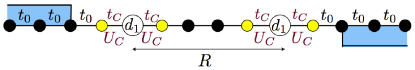
Figure 1: (Color online) Picture of the model Eq. 1 for a system of $L=14$ sites and $R=5$. The shaded light blue areas indicate the presence of the bias (Eq. 7).

As it will be discussed in more detail in Sec. II.2, we will follow the transport process in the frame of a quantum quench, where a given initial state $|\Psi_{0}\rangle$ evolves in time under the action of a given Hamiltonian, such that the state of the system at a time $\tau$ is $|\Psi(\tau)\rangle=\exp(-i\hat{H}\tau)|\Psi_{0}\rangle$. Accordingly, the time-dependent occupations on each site are given by

$$n_{j}(\tau)\equiv\langle\Psi(\tau)|\hat{n}_{j}|\Psi(\tau)\rangle\;.$$ (5)

The current on each bond connecting nearest-neighbor sites can be obtained as:

$$I_{j}=i\frac{e}{\hbar}t_{j}\langle\Psi(\tau)|(\hat{c}^{\dagger}_{j}\hat{c}_{j+1}-\hat{c}^{\dagger}_{j+1}\hat{c}_{j})|\Psi(\tau)\rangle\;,$$ (6)

where $e$ is the electron charge, $t_{j}$ is the hopping on the bond connecting sites $j$ and $j+1$.

The results presented in this work are obtained with t-DMRG White and Feiguin (2004); Daley et al. (2004); Schmitteckert (2004b); Schollwöck (2011). We typically simulate systems with $L\sim 100$ sites. In order to implement the time evolution, we use the Trotter decomposition Daley et al. (2004); White and Feiguin (2004); Al-Hassanieh et al. (2006). Our code is adaptive Daley et al. (2004); White and Feiguin (2004); Al-Hassanieh et al. (2006), meaning that the number of states used at each time step changes dynamically keeping the discarded weight below a given threshold. The maximum number of states used in our computation is $m\sim 1000$ and the discarded weight $\varepsilon$ is kept below $\sim 10^{-7}$. In the absence of interactions we employ also exact diagonalization. Comparing the latter and DMRG for typical values of $m$ and $L$ we find that the relative error of the occupations is less than $10^{-4}$ for times $\lesssim 40\hbar/t_{0}$, while for the currents it is always less than $10^{-3}$ in the same interval of time.

II.2 Quench schemes

In order to initiate transport processes in the system described by Eq. (1), a bias $\Delta V$ has to be applied on the left and the right lead. It is described by:

$$\hat{H}_{\rm B}=\frac{\Delta V}{2}\left(\sum_{j=1}^{d_{1}-1}\hat{n}_{j}-\sum_{j=d_{2}+1}^{L}\hat{n}_{j}\right)\;.$$ (7)

As previously discussed for a single impurity Branschädel et al. (2010a), we can start with the ground state of ${\hat{H}}_{\mbox{\footnotesize chain}}$ and follow the evolution of the system dictated by a Hamiltonian ${\hat{H}}_{\mbox{\footnotesize chain}}+H_{\rm B}$. We denote such a procedure scheme (A). In such a scheme, however, the bounded nature of the spectrum of a lattice model becomes evident whenever the bias exceeds the bandwidth. In that case, there are no states available for transport through the system, as shown in Fig. 2 (the determination of the currents depicted will be discussed in detail in Sec. II.3).

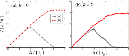
Figure 2: (Color online) I-V characteristics for a system with one (a) and two impurities (b). Black empty circles and red full squares refer to quench schemes (A) and (B) respectively. All the curves are obtained with $L=100$, except for $R=7$, scheme (A), for which $L=300$ sites are used. Data for $t_{\rm C}=0.8t_{0}$ and $U_{\rm C}=0.0$. The current is shown in absolute value.

It was suggested previously Boulat et al. (2008); Branschädel et al. (2010a), that in order to avoid such an artifact of a lattice model, the opposite scheme can be used, namely, the initial state is the ground state of ${\hat{H}}_{\mbox{\footnotesize chain}}+H_{\rm B}$, and the evolution is studied switching off $H_{\rm B}$. As shown in Fig. 2, such a quench scheme leads to a saturation of the attained current, with similar behavior for a single impurity or two of them with a Fermi sea inbetween. The current in scheme (B) saturates at large values of the bias, because of the finite bandwidth of the system Cini (1980); Branschädel et al. (2010a). For $\Delta V$ smaller than half the bandwidth, both schemes lead to the same result. Moreover, for the whole range of biases studied in the one-impurity case Boulat et al. (2008), the I-V curves can be brought in this way to coincide with analytical results from conformal field theory.

In scheme (B) the initial state is characterized by a particle imbalance between the left and right lead, due to the presence of the bias, and the distribution of particles in the central region is not uniform. However, we find $\rho_{\rm c}=\rho$ if the system is at half filling. In the other cases there is a discrepancy which can be controlled by performing a finite-size scaling.

In the rest of the work we choose quench scheme (B) because it avoids the artifact introduced by a bounded spectrum.

II.3 Time averages

As already discussed in the Refs. Branschädel et al., 2010a and Nuss et al., 2013 in the case of a single quantum dot, the time evolution of a current in a finite system is affected in various ways. On the one hand, right after switching the bias on (or off), there is a transient time, where the current grows from zero to a quasi-stationary state. On the other hand, at long times, the current bounces back at the ends of the system.

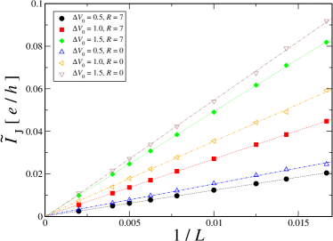
Figure 3: (Color online) Finite size scaling of the oscillation amplitudes $\tilde{I}_{\rm J}$ from cosine fits as discussed in main text, extracted from the left-contact current $I_{c1}$. Data refer to a system with $t_{\rm C}=0.8t_{0}$, $U_{\rm C}=0$, $R=0$ (empty symbols) and $R=7$ (full symbols).

In the intermediate quasi-stationary state, periodic variations previously denoted Josephson oscillations Branschädel et al. (2010a), due to their similarity with the ones in a Josephson junction, appear with a period $T_{\rm J}\equiv 1/\nu_{\rm J}=2\pi/\Delta V$ determined by the bias, with an amplitude that vanishes Branschädel et al. (2010a) as $1/L$. Hence, in the free case one can extract an approximant to the steady-state current fitting the Josephson oscillations with a cosine function Branschädel et al. (2010a) of the form $I_{\alpha}(\tau)=\tilde{I}+\tilde{I}_{\rm J}\cos(2\pi\tau/T_{\rm J}+\tilde{\varphi})$, where $\alpha=c_{1}$ or $c_{2}$ denotes the left or right contact, and the free parameters of the fit are $\tilde{I}$, $\tilde{I}_{\rm J}$ and $\tilde{\varphi}$.

In the case of two impurities without interaction we find the same time scales, with minor differences. In particular the transient time also depends on the distance between the two impurities, and the amplitude of the Josephson oscillations is also affected by $R$. Nevertheless, as we show in Fig. 3, it is still possible to extract the approximant to the steady-state current by fitting the Josephson oscillations as mentioned above, obtaining an amplitude that also vanishes in the thermodynamic limit.

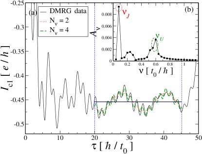
Figure 4: (Color online) (a) Black continuous line: left-contact current $I_{c1}$ for a system of $L=100$ with two impurities at distance $R=7$, $t_{\rm C}=0.8t_{0}$, $\Delta V=0.5t_{0}$, and $U_{\rm C}=5t_{0}$. Horizontal continuous straight line: zero frequency component of the DFT in the interval $[20,45]$ (delimited by vertical dashed lines). (b): DFT of the black curve in (a). The red dotted curve in (a) corresponds to $N_{\nu}=2$ frequencies: the zero frequency component and the Josephson frequency $\nu_{\rm J}$. The green dashed curve in (a) is found using also the frequencies framed by the dashed line in (b).

In the presence of interaction, both for one and two impurities, additional frequencies emerge. In Fig. 4 we show the current on the left contact for $U_{C}=5t_{0}$ as an example, where additional oscillations superimposed to the Josephson oscillations (they have in this case a period $T_{\rm J}\sim 12.6\hbar/t_{0}$) are clearly visible. In order to deal with the appearence of several frequencies, we perform a discrete Fourier transform (DFT) by first identifying an interval of time where the evolution is quasi-stationary, with a duration that is an integer number of Josephson periods $T_{\rm J}$. Then we do a reconstruction of the current by picking up only the few most important frequencies from the DFT, which always include the zero frequency component (the approximant to the steady-state current), the Josephson frequency $\nu_{J}$, and the one due to interaction with the highest Fourier weight $\nu_{U}$, as displayed in Fig. 4, where the quality of such a reconstruction can be seen for two different numbers of frequencies considered. We associate to the approximant to the steady-state current the uncertainty:

$$\Delta I\equiv\frac{1}{M}\sqrt{\sum_{i=1,M}\left(I(\tau_{i})-\tilde{I}(\tau_{i})\right)^{2}}\;,$$ (8)

where $\tau_{i}$, with $i=1,M$, are the equally spaced times lying in the interval where the DFT is performed, $I(\tau_{i})$ is the current measured at $\tau_{i}$ and $\tilde{I}$ is the reconstructed current. The uncertainty $\Delta I$ is typically within the size of the symbols in our plots.

By using the procedure described above we reproduce in Fig. 5 the I-V characteristics of a single impurity in the full range of interactions and biases with excellent agreement with the original work Boulat et al. (2008).

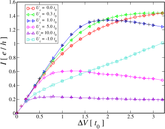
Figure 5: (Color online) I-V characteristics of a system at $t_{\rm C}=0.5t_{0}$ with quench scheme (B). The crosses are data from Ref. Boulat et al., 2008, the symbols are those obtained with our code (the parameters of our simulations are $L=96$, $m=600$ states, discarded weight $\varepsilon<10^{-7}$).

III Results

III.1 Phase relations

As is well known, the RKKY interaction is an indirect exchange interaction between two localized spins mediated by the surrounding electrons of the Fermi sea Ruderman and Kittel (1954); *Kasuya_PTP56; *Yosida_PR57; *VanVleck_RMP62; *Kittel. In the present case, since we are dealing with spinless fermions, only a coupling to the density will result. The RKKY interaction depends on the distance between the impurities $R$ via $2k_{\rm F}$ oscillations Ruderman and Kittel (1954); *Kasuya_PTP56; *Yosida_PR57; *VanVleck_RMP62; *Kittel and is expected to induce correlations between the densities on the two dots and, consequently, on the currents in the contacts. We now show that the occupations on the dots closely fulfill the predictions of the RKKY interaction, first considering half-filling, and then a case away from it. The same correlations are also visible in the currents, but with a phase shift.

We consider first the system at half-filling, i.e. $N/L=0.5$ in the free case and concentrate on the quasi-steady regime. In the left panels of Fig. 6 we show the occupations on the two quantum dots.

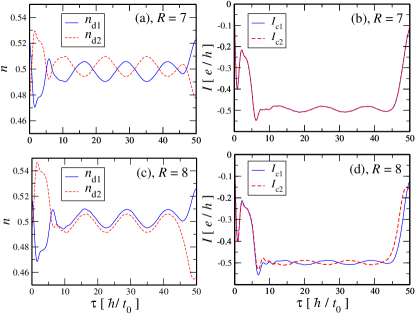
Figure 6: (Color online) Panels (a) and (c): time evolution of the number of particles on the left (blue continuous line) and right dot (red dashed line); panels (b) and (d): time evolution of the left-contact (blue continuous line) and right-contact (red dashed line) currents. Data for a system of $L=100$, $t_{\rm C}=0.8t_{0}$, $\Delta V=0.5t_{0}$, half-filling, quench scheme (B) and $U_{\rm C}=0$.

They oscillate with the Josephson frequency $\nu_{\rm J}$, which characterizes also the current (see Sec. II.3). More interestingly we observe that when $R$ is odd the densities oscillate in opposition of phase, while if $R$ is even they oscillate in phase. This is a regular pattern which we find in all the range of $R$ considered. This behavior is compatible with the $2k_{\rm F}$ oscillations of the RKKY interaction, as shown by Fig. 7.

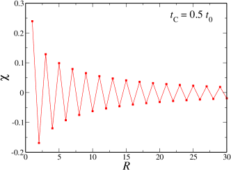
Figure 7: (Color online) Static susceptibility connecting the dots at sites $d_{1}$ and $d_{2}$ for $t_{C}=0.5t_{0}$ for half-filling.

There it can be seen that the static susceptibility, that displays $2k_{F}$ oscillations as a function of $R$, is positive for $R$ odd and negative for $R$ even. Therefore, for $R$ odd the densities at the dots experience an effective repulsive interaction, while for $R$ even it is attractive.

If we now move to the right panels of Fig. 6 we find the opposite situation. When $R$ is odd the currents oscillate in phase (they are exactly equal in this case) and when $R$ is even they are in opposition of phase. In the latter case averaging the currents of the two contacts cancels out the oscillations. This effect is visible only in the quasi-stationary regime, as we can see from the left panels of Fig. 6. The phase-shift between densities and currents can be undertstood by noticing that when the mean density on a dot increases, transfer of a particle to (from) the dot is suppressed (enhanced). Then, for $R$ odd, while one dot has a higher density, the other has a lower one. Considering the current on the links to the left of $d_{1}$ and to the right of $d_{2}$, charge flow is enhanced on both links when $d1$ has an increased density and $d_{2}$ a reduced one, while in the opposite case current is suppressed. On the other hand, when $R$ is even, both dots have an enhanced density or a suppressed one, such that when charge can be transferred on one link, the current is suppressed on the other.

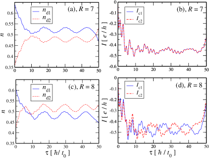
Figure 8: (Color online) Same as Fig. 6 but for $U_{\rm C}=5t_{0}$.

Although the evolution of the current is more involved in the presence of interaction due to the appearence of additional oscillations, the same qualitative considerations hold also at half-filling for $U_{\rm C}\neq 0$ . As an example, in Fig. 8 we show the currents and the densities in the presence of interaction, namely at $U_{\rm C}=5t_{0}$. The behavior of the densities is very clear and analogous to the free case. However, the interaction enhances the amplitude of the oscillations as can be seen comparing Figs. 6 and 8. In spite of the interaction, it is clearly visible that for the odd-$R$ case the currents are exactly equal and for even $R$ an opposition in phase is evident.

Next we consider a situation away from half filling. In this case, however, already in the absence of interactions and for values of $t_{\rm C}$ different from $t_{0}$, the density in the central region (composed of the sites $d_{1}+1$ to $d_{2}-1$) $\rho_{c}$ does not in general coincide with $\rho=N/L$, in contrast to the half filling case. Yet, as we discuss below, an examination of the phase differences between the densities at the quantum dots and currents across them displays a pattern that can be consistently assigned to the RKKY interaction. As an example we show in Fig. 9 the density and the current for a system of $L=400$ accomodating a number of particles $N$ such that $\rho_{c}$, the density in the internal region, is as close as possible to quarter filling for each $R$ considered there. In particular we chose $N=105$, which gives $\rho_{c}=0.246$ for $R=9$. Figures 9 (a), (c), and (e) display the oscillations of the density on each dot as a function of time. The density between them being approximately 1/4, a phase difference $\Delta\phi\simeq 3\pi/2$ is expected, while the actual value is 1.23 $\pi$. Such a deviation corresponds to a departure of the mean density in that region of around 10%. In spite of the slight deviation from the expected value of the phase difference for a given $R$, the periodicity four expected from the RKKY susceptibility at $k_{\rm F}=\pi/4$ is indeed found on going from $R=7$ to $R=11$ ($\Delta\phi\simeq 1.26\pi$). This fact is, moreover, clearly seen on Figs. 9 (b), (d), and (f), where the current through the dots is plotted.

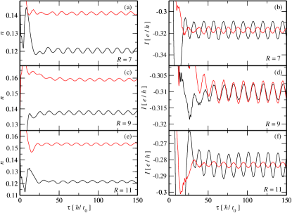
Figure 9: (Color online) Panels (a), (c), and (e): time evolution of the number of particles on the left (black line) and right dot (red line); panels (b), (d), and (f): time evolution of the left-contact (black line) and right-contact (red line) currents. Data for a system of $L=400$, $t_{\rm C}=0.8t_{0}$, $N=98$, $\Delta V=0.5t_{0}$, quench scheme (B) and $U_{\rm C}=0$.

In the interacting case the presence of additional frequencies has to be taken into account, as already discussed for half-filling. Moreover, we have to consider also the departure of $\rho_{c}$ from $\rho$. In Fig. 10 we show an example of the instantaneous densities and currents with $U_{\rm C}=1.0t_{0}$. In order to tune $\rho_{c}$ as close as possible to quarter filling, we chose to work with $N=24$ particles, giving $\rho_{c}=0.252$ and $\rho_{c}=0.248$ for $R=5$ and $R=7$ respectively. Performing a discrete Fourier transform on an integer number of Josephson periods (also considering different choices of the initial and final times), we computed the reconstructed densities and currents using only the Josephson frequency. For the time interval shown in Fig. 10 the phase between the densities and the currents changes by roughly $\pi$ going from $R$ to $R+2$, in reasonable agreement with the free case. However, due to the difficulty to fix the density in the central region, the results away from half-filling do not allow for a clear identification of phase changes as expected on the basis of the RKKY interaction.

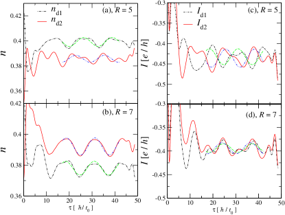
Figure 10: (Color online) Panels (a) and (c): time evolution of the number of particles on the left (black dash-dotted) line) and right dot (red line); panels (b) and (d): time evolution of the left-contact (black dash-dotted line) and right-contact (red line) currents. The blue dash-dash-dotted and the green dashed lines in each panel are the reconstructed quanties, obtained retaining only the component of the DFT in the interval $\tau\in[17,42.13]\hbar/t_{0}$ corresponding to Josephson frequency. Data for a system of $L=100$, $t_{\rm C}=0.8t_{0}$, $N=24$, $\Delta V=0.5t_{0}$, quench scheme (B) and $U_{\rm C}=2.0t_{0}$.

The previous results were obtained on systems where the leads are finite, and hence allowed for a change in density. It would be on the other hand interesting to see, how much the results change in the limit of macroscopic leads. While, as shown in Fig. 3, it should be expected that the Josephson oscillations vanish, macroscopic leads will provide also an essentially infinite reservoir of fermions. It is therefore interesting to see how such reservoirs affect the region between the dots. Although it is not possible to answer this question numerically, we can obtain an insight by considering a non interacting system with infinite leads within the Keldysh formalism  Rammer (2007); Haug and Jauho (2008); Kennes et al. (2012) in the wide-band limit, where the density of states in the leads is considered constant. Following Kennes et al. Kennes et al. (2012), we choose a quench scheme where the bias is always present, the coupling to the leads is switched on at time $\tau=0$ and the sites in the central region are initially empty. The wide-band limit is reached taking both the hopping in the contacts and the bias much smaller than the hopping in the leads, so $t_{\rm C}\ll t_{0}$ and $\Delta V\ll t_{0}$. For the Fermi sea, instead of $t_{0}$, we take a hopping $t^{\prime}_{\rm C}$ of the same order of $t_{\rm C}$, in particular we choose $t_{\rm C}=0.1t_{0}$ and $t^{\prime}_{\rm C}=0.12t_{0}$ and $\Delta V=0.01t_{0}$. In Fig. 11 we show our results for two impurities obtained within the Keldysh formalism, where we compute the current leaving the left lead ($I_{c1-1}$) and entering the right lead ($I_{c2+1}$).

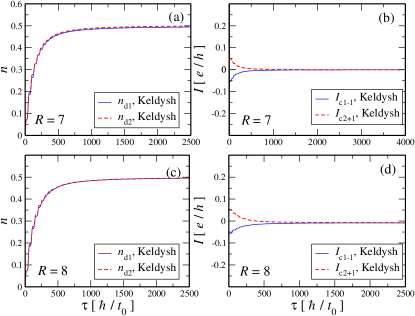
Figure 11: (Color online) Panels (a) and (c): time evolution of the number of particles computed within the Keldysh formalism on the left (blue continuous line) and right dot (red dashed line); panels (b) and (d): time evolution of the left-lead (blue continuous line) and right-lead (red dashed line) currents. Data for $t_{\rm C}=0.1t_{0}$, $t^{\prime}_{\rm C}=0.12t_{0}$ (see main text) and $\Delta V=0.01t_{0}$. Panels (a) and (b): $R=7$, panels (c) and (d): $R=8$.

We have also checked (not shown) that we obtain an excellent approximation of the curves shown in Fig. 11 by taking tight-binding leads in system of large size with the same values of $t_{\rm C}$, $t^{\prime}_{\rm C}$ and $\Delta V$, as long as the time $\tau$ is smaller than the reflection time (see Sec. II.3). Both the occupations on the dots and the currents shown in Fig. 11 reach their steady state value after a transient and, as expected, no Josephson oscillations are observed. In both cases, $R=7$ and $R=8$, the steady-state value of the density is close to half-filling, independently of the initial filling and of the size of the region between the dots. Therefore, in the wide-band limit, the relevant case turns out to be that of half-filling. The relaxation of the density to the steady state can be fitted with an exponential of the form $n(\tau)=n_{0}(1-\exp(-\alpha\tau))$ giving $\alpha=E_{\rm WB}/6.1$ and $\alpha=E_{\rm WB}/8.3$ for $R=7$ and $R=8$ respectively, where we have introduced the energy scale Kennes et al. (2012) $E_{\rm WB}\equiv 4t_{\rm C}^{2}/t_{0}$. The time scale $1/E_{\rm WB}$ dictates the exponential relaxation of the single impurity i.e. $n(\tau)=0.5(1-\exp(-E_{\rm WB}\tau))$, and with $t_{\rm C}=0.1t_{0}$ has the value $1/E_{\rm WB}=25\hbar/t_{0}$. If we now consider the tight-binding case of Fig. 6, corresponding to $t_{\rm C}=0.8$, we find $1/E_{\rm WB}=0.39\hbar/t_{0}$. This is precisely the time scale over which the currents of Fig. 6 ramp from zero to the quasi-steady state regime where we observe the Josephson oscillations. Moving back to Fig. 11, the values of the steady-state current are $I\sim 6\cdot 10^{-4}e/h$ for $R=7$ and $I\sim 8\cdot 10^{-3}e/h$ for $R=8$. Although these values differ significantly from each other, this difference is negligible with respect to the uncertainty with which the current can be accessed for example in the case of Fig. 6. The smaller order of magnitude of the steady-state currents of Fig. 11 with respect to those of Fig. 6 can be understood taking into account that the bias is fifty times smaller here and also $t_{\rm C}\ll t_{0}$.
The phases characterizing the time evolution of the density and of the current described above reveal the effect of the RKKY interaction on the slow dynamics of the Josephson oscillations, giving rise to sustained and controllable oscillations of the densities and of the currents in finite size systems at half-filling. This fact may turn out to be observable in experiments focused on quantum dots set-ups in mesoscopic systems. Indeed there have been proposals of simulating quantum impurity systems and transport properties in cold atom systems Recati et al. (2005); Knap et al. (2012). The first experimental progress done so far in this direction is the realization of a mesoscopic conducting channel in a cloud of Litihum atoms, performed by Brantut and collaborators Brantut et al. (2012).

III.2 Average current as a function of the distance

III.2.1 Free case

The results shown above indicate that the dynamics of the current and the density is regulated by $2k_{\rm F}$ oscillations due to the RKKY interaction. We now investigate how the behavior of the steady-state current is affected by the distance between the impurities and the Fermi momentum. In Fig. 12 we show the approximant to the steady-state current in absence of interaction as a function of the distance between the impurities.

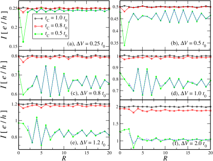
Figure 12: (Color online) Approximant to the steady state current as a function of the distance between noninteracting impurities for a system of $L=200$ sites for different values of the contact hopping, quench scheme (B) and $U_{\rm C}=0.0$. Blue dashed line: Landauer-Büttiker formula (cf. Eq. 11) applied to the case $t_{\rm C}=0.5t_{0}$. From top to bottom, left to right: $\Delta V=0.25,0.5,0.8,1.0,1.2,2.0t_{0}$. (The current is plotted in absolute value.).

The simplest case is $t_{\rm C}=t_{0}$, for which the data of Fig. 12 show very small variations as a function of $R$, which however are only a finite-size effect. On the other side, from Fig. 12 we see that the curves with $t_{\rm C}=0.5t_{0}$ are the most sensitive to $R$, showing pronounced fluctuations. Furthermore, for $t_{\rm C}=0.5t_{0}$, there is a range of $R$ where the oscillations have the largest amplitude. This range changes with $\Delta V$. As an example, for $\Delta V=0.5t_{0}$ the range is given approximately by $R\sim 7\div 19$, while for $\Delta V=0.8t_{0}$ by $R\sim 4\div 13$. Moreover, the period of these oscillations is typically $R=2$.

Following the Landauer-Büttiker approach Büttiker (1986); Blanter and M (2000), we now show that the patterns of the current of Fig. 12 can be understood in terms of the transmission properties for a single particle. Indeed, the physical mechanism at the root of the flow of current is that the dot, characterized by $t_{\rm C}\neq t_{0}$, is an effective tunnel barrier with an energy-dependent transmission probability $p_{s}(\epsilon)$ (where the subscript $s$ stands for single). The presence of two dots requires the combination of the transmission propabilities in order to compute the total probability $p_{d}(\epsilon)$ (the subscript $d$ standing for double). The transmission probability through a single dot is given by Branschädel et al. (2010b):

$$p_{s}(\epsilon)=\frac{1-\epsilon^{2}/(4t_{0}^{2})}{1+\epsilon^{2}(t_{0}^{2}-2t_{\rm C}^{2})/(4t_{\rm C}^{4})}\;.$$ (9)

The total transmission probability can be obtained using the transfer matrix approach R.A. Molina et al. (2005); Blanter and M (2000) and gives:

$$p_{d}=\frac{p_{s}^{2}}{1+(1-p_{s})^{2}-2(1-p_{s})\cos(2k(\epsilon)R+2\phi)}\;,$$ (10)

where $\phi=kb$ and $b$ is the size of the single tunnel barrier. In our case we have that $t_{\rm C}$ is present on three sites (the dot and its nearest-neighbors), so $b=3$. The expression for the combined probability eq. (10) is valid provided $R\geq 3$. Indeed, for $R=1,2$ one has to consider a single barrier of size $b=4,5$ respectively. In order to obtain the average current, one has to integrate the transmission probability over the energies of current-carrying states. This yields Büttiker (1986):

$$I(\Delta V)=\int_{\epsilon_{\rm F}-\Delta V/2}^{\epsilon_{\rm F}+\Delta V/2}d\epsilon\;p_{d}(\epsilon)\;.$$ (11)

Our results for $t_{\rm C}=0.5t_{0}$ are the blue dashed lines of Fig. 12. We observe that there is a very good agreement with the current obtained by doing the time average.

In Fig. 13 we consider a system with filling $\rho_{c}\simeq 0.25$ and show the approximant to the steady-state current (computed for a system of $L=400$ sites) and the prediction of Eq. 11 for $k_{\rm F}=0.25.$

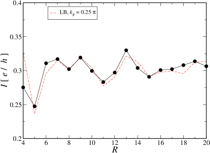
Figure 13: (Color online) Approximant to the steady state current for a system with $t_{\rm C}=0.8t_{0}$, $\Delta V=0.5t_{0}$ and scheme (B) for $L=400$ (black dots) and Landauer-Büttiker prediction from Eq. 11 for $k_{\rm F}=0.25\pi$. (red dashed line).

In spite of the difficulties in setting a definite density in the region between the dots away from half filling, a rather good agreement with the Landauer-Büttiker formula is obtained, with small deviations due to fluctuations of the density in the central region on going from one value of $R$ to another.

III.2.2 Interacting case

We start by considering the effect of a small interaction, namely $U_{\rm C}=1.0t_{0}$, and we choose $t_{\rm C}=0.5t_{0}$ in order to probe if and how the interaction affects the resonances (Fig. 14). From the comparison with the free case we can see first that the current is enhanced, an effect that becomes stronger at larger values of the bias. The enhancement of the current by interaction is also observed in the one impurity case Boulat et al. (2008) (see Fig. 5 for small $U_{\rm C}\lesssim t_{0}$ and $\Delta V\lesssim 2t_{0}$). Furthermore, it can be seen that the resonances observed in the free case are suppressed. The deviation of the conductance from the Landauer-Büttiker combination of probabilities for small values of the interaction was already observed in Ref.R.A. Molina et al., 2005.

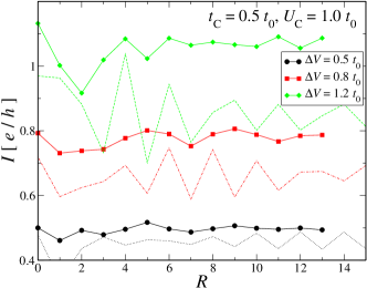
Figure 14: (Color online) Approximant to the steady-state current as a function of the distance between the impurities $R$ for a system of $L=100$ sites with $U_{\rm C}=1.0t_{0}$ for different values of the bias and quench scheme (B). The currents in the non-interacting case (dotted, dash-dotted and dashed lines show the current and correspond to $\Delta V=0.5,0.8,1.2t_{0}$ respectively) are shown as reference. The uncertainty on the value of the average current $\Delta I$ as discussed in Sec. II.3 is within the size of the symbols in the plot. (The current is plotted in absolute value.)

In Fig. 15 we show our results for the approximant to the steady-state current with increasing values of the interaction. While the current does not vary significantly for values of $U_{C}$ lower than the band-width, a qualitatively different behavior appears when $U_{C}$ is larger than $4t_{0}$. For $U_{\rm C}=6,10t_{0}$ and $R\gtrsim 6$ we interestingly find that the current oscillates as a function of the distance with periodicity two, with a rather large amplitude, which is typical of RKKY oscillations at half-filling.

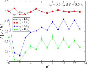
Figure 15: (Color online) Approximant to the steady-state current as a function of the distance between the impurities $R$ for a system of $L=100$ sites with $t_{\rm C}=0.5t_{0}$ and $\Delta V=0.5t_{0}$ for different values of the interaction and quench scheme (B). In some cases the approximant to the steady-state current is strongly sensitive on the chosen boundaries of the stationary regime where the DFT is performed. The resulting different values of the current lie inside the error bars. (The current is plotted in absolute value.)

The same behavior is also confirmed if we change the contact hopping, for example with $t_{\rm C}=0.8t_{0}$ (Fig. 16). In Fig. 12 we saw that without interaction the current is in this case almost independent on $R$, because the single tunnel barrier has a transmission coefficient close to unity (see Eq. 9). On the contrary, comparing Figs. 15 and  16 we see that the approximant to the steady-state current oscillates with $R$ for both values of $t_{C}$ with the same pattern if the interaction is large enough, i.e. $U_{\rm C}\gtrsim 5.0t_{0}$, hinting at a signature of the RKKY interaction. It is also remarkable that the maxima of the current are of the same order as for the single-impurity case. It is to be emphasized however, that even-odd oscillations of the conductance have also been observed in a system with an impurity separated by a non-interacting lead Weinmann et al. (2008) from a non-interacting potential scatterer.

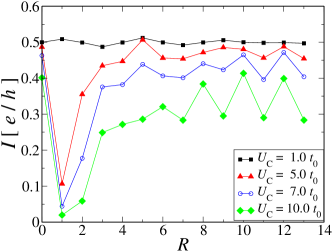
Figure 16: (Color online) Approximant to the steady-state current as a function of the distance between the impurities $R$, in the presence of a small bias $\Delta V=0.5t_{0}$ for a system of $L=100$ sites for different values of the interaction and $t_{\rm C}=0.8t_{0}$. The uncertainty on the value of the average current $\Delta I$ as discussed in Sec. II.3 is within the size of the symbols in the plot. (The current is plotted in absolute value.)

To test the dependence of the oscillations as a function of $R$ on filling would be in principle desirable. However, at low filling the current is drastically suppressed in the presence of large interactions. Indeed, by considering for example quarter filling with $L=100$ sites, already at $U_{\rm C}=5.0t_{0}$ the current is characterized by high-frequency oscillations around zero (data not shown), thus precluding the observation of possible RKKY oscillations. Recalling also the problem of the deviation of $\rho$ from $\rho_{c}$ discussed in the previous sections, regimes away from half-filling would require the investigation of much larger sizes, in order both to control precisely $\rho_{c}$ and to avoid strong finite-size effects present in very dilute systems with large $U_{\rm C}$, beyond the present computational capabilities.

III.3 I-V characteristics

For the case of one impurity, the I-V characteristics is characterized by a regime of negative conductance, where the current decreases as a power-law, with interaction dependent exponents Boulat et al. (2008) (see also Fig. 5). Furthermore, it is possible to define an universal energy scale $T_{\rm B}$ Boulat et al. (2008), which depends on $t_{\rm C}$. At the self-dual point it gives rise to a universal power-law decay, i.e., by rescaling different I-V characterstics with $T_{\rm B}$ they all sit on the same curve Boulat et al. (2008). In the case of two impurities we also find a regime of negative conductance, as we show in Fig. 17.

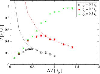
Figure 17: (Color online) Approximant to the steady-state current as a function of the bias $\Delta V$, with $U_{\rm C}=2.0$, $R=7$ and $L=100$ sites for different values of the contact hopping $t_{\rm C}$. Black empty squares, red full dots, green triangles correspond to $t_{\rm C}=0.2,0.3,0.5t_{0}$ respectively, while dashed lines are power-law fits. (The current is plotted in absolute value.)

We observe that the behavior of the current is in some cases not very smooth. This is due to finite-size effects. The curves of Fig. 17 show that the current first increases approximately linearly, has a maximum and then decreases. However, in order to verify if a power law may describe the sector with a negative conductance, as in the case of a single quantum dot Boulat and Saleur (2008), an extended range in values of the bias are necessary. In the case of two dots coupled by a Fermi sea, such a range in values of $\Delta V$ becomes very demanding in terms of the number of DMRG states that have to be kept for a reasonalbe accuracy, such that a quantitative answer cannot be given to this question.

IV Summary

By studying the time dependence of the current and the density in a one-dimensional chain in the presence of two interacting resonant levels, we tested the interplay of the RKKY interaction and the characteristics of the quantum dots, concerning the dynamical behavior in a finite system as well as the approximant of the steady-state current.

Focusing on the time evolution, we found that, at finite size, the evolution of the current in the contacts and the occupations of the dots are characterized by oscillations, whose period depends on the applied bias as in the single dot case Branschädel et al. (2010a), but interrelated in a way that depends on the size of the Fermi sea. In fact, we show that the densities on the dots oscillate with a relative phase which depends on the Fermi momentum of the Fermi sea and on the distance between the impurities, as expected for the RKKY interaction. An analogous behavior is found for the time evolution of the currents in the contacts, which are related to those of the density, but phase shifted with respect to them. While at half-filling those correlations can be clearly seen, away from half-filling it is necessary to precisely control the $k_{F}$ by appropriately tuning the global density $\rho$, since the latter does not coincide in general with the density in the central region $\rho_{c}$, rendering the comparison for different values of $R$ difficult. The phase relations described above can be exploited in experimental measurements in mesoscopic systems. As mentioned before, experimental investigation of transport in cold atomic systems Brantut et al. (2012); Killi and Paramekanti (2012); Killi et al. (2012); Knap et al. (2012), would be an interesting set-up, where the variations of the density in the quantum dots could be accessed directly. In the thermodynamic limit the oscillations of the current and the density vanish, as we have shown by an explicit extrapolation, and with analytic calculations in the wide-band limit.

We have also studied the approximant to the steady state current, and its oscillations as a function of the distance between the dots. In the free case we identified resonances that can be traced back to the resonances affecting the transmission coefficients of a single particle propagating freely in the system. Turning interactions on the resonances are suppressed. However, for large values of the interaction we observe at half-filling rather large oscillations of the current as a function of the distance with periodicity two. This matches $2k_{\rm F}$ oscillations, hinting at the influence of the RKKY interaction. Finally, we focused on the I-V characteristics , finding a region of negative conductance, in analogy with the one-impurity case.