Efficient Support for Mode-Directed Tabling in the YapTab Tabling System

Abstract

Mode-directed tabling is an extension to the tabling technique that supports the definition of mode operators for specifying how answers are inserted into the table space. In this paper, we focus our discussion on the efficient support for mode directed-tabling in the YapTab tabling system. We discuss 7 different mode operators and explain how we have extended and optimized YapTab’s table space organization to support them. Initial experimental results show that our implementation compares favorably with the B-Prolog and XSB state-of-the-art Prolog tabling systems.

1 Introduction

Tabling [1] is a recognized and powerful implementation technique that solves some limitations of Prolog’s operational semantics in dealing with recursion and redundant sub-computations. Tabling based models are able to reduce the search space, avoid looping, and always terminate for programs with the bounded term-size property. Tabling consists of saving and reusing the results of sub-computations during the execution of a program and, for that, the calls and the answers to tabled subgoals are stored in a proper data structure called the table space. In a traditional tabling system, all the arguments of a tabled subgoal call are considered when storing answers into the table space. When a new answer is not a variant of any answer that is already in the table space, then it is always considered for insertion. Therefore, traditional tabling systems are very good for problems that require storing all answers. Mode-directed tabling [2] is an extension to the tabling technique that supports the definition of selective criteria for specifying how answers are inserted into the table space. The idea of mode-directed tabling is to use mode operators to define what arguments should be used in variant checking in order to select what answers should be tabled.

In a traditional tabling system, to evaluate a predicate $p/n$ using tabling, we just need to declare it as ‘$table~{}p/n$’. With mode-directed tabling, tabled predicates are declared using statements of the form ‘$table~{}p(m_{1},...,m_{n})$’, where the $m_{i}$’s are mode operators for the arguments. Implementations of mode-directed tabling are already available in systems like ALS-Prolog [2] and B-Prolog [3], and a restricted form of mode-directed tabling can be also recreated in XSB Prolog by using answer subsumption [4].

In this paper, we focus our discussion on the efficient implementation of mode directed-tabling in the YapTab tabling system [5], which uses tries [6] to implement the table space. Our implementation uses a more general approach to the declaration and use of mode operators and, currently, it supports 7 different modes: index, first, last, min, max, sum and all. To the best of our knowledge, no other tabling system supports all these modes and, in particular, the sum mode is not supported by any other system. Experimental results, using a set of benchmarks that take advantage of mode-directed tabling, show that our implementation compares favorably with the B-Prolog and XSB state-of-the-art Prolog tabling systems.

The remainder of the paper is organized as follows. First, we introduce some background concepts about tabling. Next, we describe the mode operators that we propose and we show some small examples of their use. Then, we introduce YapTab’s table space organization and describe how we have extended it to efficiently support mode-directed tabling. At last, we present some experimental results and we end by outlining some conclusions.

2 Tabled Evaluation

In a traditional tabling system, programs are evaluated by storing answers for tabled subgoals in an appropriate data structure called the table space. Similar calls to tabled subgoals are not re-evaluated against the program clauses, instead they are resolved by consuming the answers already stored in the corresponding table entries. During this process, as further new answers are found, they are stored in their tables and later returned to all similar calls.

Figure 1 illustrates the execution of a tabled program. The top left corner of the figure shows the program code and the top right corner shows the final state of the table space. The program defines a small directed graph, represented by two edge/2 facts, with a relation of reachability, defined by a path/2 tabled predicate. The bottom of the figure shows the evaluation sequence for the query goal path(a,Z). Note that traditional Prolog would immediately enter an infinite loop because the first clause of path/2 leads to a variant call to path(a,Z).

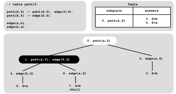
Figure 1: An example of a tabled evaluation

First calls to tabled subgoals correspond to generator nodes (nodes depicted by white oval boxes) and, for first calls, a new entry, representing the subgoal, is added to the table space (step 0). Next, path(a,Z) is resolved against the first matching clause calling, in the continuation, path(a,Y) (step 1). Since path(a,Y) is a variant call to path(a,Z), we do not evaluate the subgoal against the program clauses, instead we consume answers from the table space. Such nodes are called consumer nodes (nodes depicted by black oval boxes). However, at this point, the table does not have answers for this call, so the computation is suspended.

The only possible move after suspending is to backtrack and try the second matching clause for path(a,Z) (step 2). This originates the answer {Z=b}, which is then stored in the table space (step 3). At this point, the computation at node 1 can be resumed with the newly found answer (step 4), giving rise to one more answer, {Z=a} (step 5). This second answer is then also inserted in the table space and propagated to the consumer node (step 6), which originates the answer {Z=b} (step 7). This answer had already been found at step 3. Tabling does not store duplicate answers in the table space and, instead, repeated answers fail. This is how tabling avoids unnecessary computations, and even looping in some cases. A new answer is inserted in table space only if it is not a variant of any answer that is already there. Since there are no more answers to consume nor more clauses left to try, the evaluation ends and the table entry for path(a,Z) can be marked as completed.

3 Mode-Directed Tabling

With mode-directed tabling, tabled predicates are declared using statements of the form ‘$table~{}p(m_{1},...,m_{n})$’, where the $m_{i}$’s are mode operators for the arguments. We have defined 7 different mode operators: index, first, last, min, max, sum and all. Arguments with modes first, last, min, max, sum or all are assumed to be output arguments and only index arguments are considered for variant checking. After an answer be generated, the system tables the answer only if it is preferable, accordingly to the meaning of the output arguments, than some existing variant answer. Next, we describe in more detail how these modes work and we show some examples of their use in the YapTab system.

3.1 Index/First/Last Mode Operators

Starting from the example in Fig. 1, consider now that we modify the program so that it also calculates the number of edges that are traversed in a path. Figure 2 illustrates the execution of this new program. As we can see, even with tabling, the program does not terminates. Such behavior occurs because there is a path with an infinite number of edges starting from a, thus not verifying the bounded term-size property necessary to ensure termination. In particular, the answers found at steps 3 and 7 and at steps 5 and 9 have the same answer for variable Z ({Z=b} and {Z=a}, respectively), but they are both inserted in the table space because they are not variants for variable N.

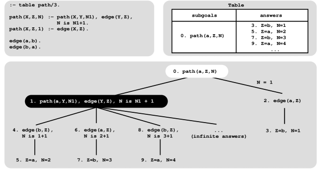
Figure 2: A tabled evaluation with an infinite number of answers

Knowing that the problem with the program in Fig. 2 resides on the fact that the third argument generates an infinite number of answers, we can thus define the path/3 predicate to have mode path(index,index,first). The index mode means that only the given arguments must be considered for variant checking. The first mode means that only the first answer must be stored. By considering this declaration, the answer {Z=b, N=3} is no longer inserted in the table and execution fails. That happens because, with the first mode on the third argument, the answer {Z=b, N=1} found at step 3 is considered a variant of the answer {Z=b, N=3} found at step 7.

The last mode implements the opposite behavior of the first mode, i.e., it always stores the last answer being found and deletes the previous one, if any. The last mode has shown to be very useful for implementing problems involving Preferences [7] and Answer Subsumption [8].

3.2 Min/Max Mode Operators

The min and max modes allow to specify a selective criteria that stores, respectively, the minimal and maximal answers found for an argument. To better understand their behavior, Fig. 3 shows an example using the min mode. The program’s goal is to compute the paths with the shortest distances. To do that, the path/3 predicate is declared as path(index,index,min), meaning that the third argument should store only the minimal answers for the first two arguments.

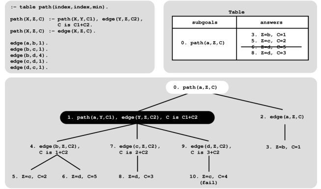
Figure 3: Using the min mode to compute the paths with the shortest distances

By observing the example in Fig. 3, we can see that the execution tree follows the normal evaluation of a tabled program and that the answers are stored as they are found. The most interesting part happens at step 8, where the answer {Z=d, C=3} is found. This answer is a variant of the answer {Z=d, C=5} found at step 6. In the previous example, with the first mode, the old answer would have been kept in the table. Here, as the new answer is minimal on the third argument, the old answer is replaced by the new answer.

The max mode works similarly, but stores the maximal answer instead. In any case, we must be careful when using these two modes as they may not ensure termination for programs without the bounded term-size property. For instance, this would be the case if, in the example of Fig.3, we used the max mode instead of the min mode.

3.3 Sum/All Mode Operators

Two other modes that can be useful are the sum and the all. The sum mode allows to sum all the answers for a given argument and the all mode allows to store all the answers for a given argument. Consider, for example, the program in Fig. 4 where the path/3 predicate is declared as path(index,index,min,all) meaning that, for each path, we want to store the shortest distance of the path (the third argument) and, at the same time, we want to store the number of edges traversed, for all paths with the same minimal distances (the fourth argument).

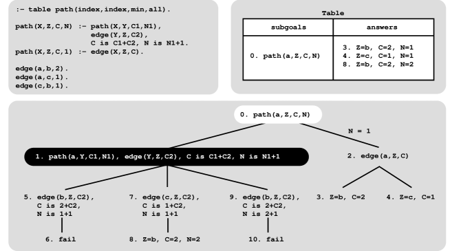
Figure 4: Using the all mode to compute the paths with the shortest distances together with the number of edges traversed

The execution tree for the program in Fig. 4 is similar to the previous ones. The most interesting part happens when the answer {Z=b, C=2, N=2} is found at step 8. This answer is a variant of the answer found at step 3 and although both have the same minimal value (C=2), the new answer is still inserted in the table space since the number of edges (fourth argument) is different.

Notice that when the sum or all modes are used in conjunction with another mode, like the min mode in the example, it is important to keep in mind that the aggregation of answers made for the sum or all argument depends on the corresponding answer for the min argument. Consider, for example, that in the previous example we had found one more answer {Z=b, C=1, N=4}. In this case, the new answer would be inserted and the answers {Z=b, C=2, N=1} and {Z=b, C=2, N=2} would be deleted because the new answer corresponds to a shorter distance, as defined by the value C=1 in the min argument.

3.4 Related Work

The ALS-Prolog [2] and B-Prolog [3] systems also implement mode-directed tabling using a very similar syntax. However, some mode operators have different names in those systems. For example, the index, first and all modes are known as +, - and @, respectively. The sum mode is not supported by any other system and B-Prolog also does not implement the last and all modes. The + (index) mode in B-Prolog is assumed to be an input argument, which means that it can only be called with ground terms. On the other hand, B-Prolog includes an extra mode, named nt, to indicate that a given argument should not be tabled and, thus, not considered to be inserted in the table space. B-Prolog also extends the mode-directed tabling declaration to include a cardinality limit that allows to define the maximum number of answers to be stored in the table space [3].

Mode-directed tabling can also be recreated in the XSB Prolog system by using answer subsumption [4]. XSB Prolog has two answer subsumption mechanisms. One is called partial order answer subsumption and can be used to mimic, in terms of functionality, the min and max modes. Consider that we want to use it with the program in Fig. 3 that computes the paths with the shortest distances. Then, we should declare the path/3 predicate as $path(\_,\_,po(</2))$ meaning that the third argument will be evaluated using partial order answer subsumption, where the predicate $</2$ implements the partial order relation. The other two arguments are considered to be index arguments.

The other XSB’s mechanism, called lattice answer subsumption, is more powerful and can be used to mimic, in terms of functionality, the other modes. To use it with the same example, we only need to change the path/3 declaration to $path(\_,\_,lattice(min/3))$. Note that the min/3 predicate must have three arguments. This is necessary since, with this mechanism, we can generate a third answer starting from the new answer and from the answer stored in the table. For example, for the shortest path problem, the predicate min/3 could be something like:

$min(Old,New,Res):-~{}Old<New\rightarrow Res=Old~{};~{}Res=New.$

4 Implementation

In this subsection, we describe the changes made to YapTab in order to support mode-directed tabling. We start by briefly presenting some background concepts about the table space organization in YapTab and then we discuss in more detail how we have extended it to efficiently support mode-directed tabling.

4.1 YapTab’s Table Space Organization

Like we have seen, during the execution of a program, the table space may be accessed in a number of ways: (i) to find out if a subgoal is in the table and, if not, insert it; (ii) to verify whether a newly or preferable answer is already in the table and, if not, insert it; and (iii) to load answers from the tables.

With these requirements, a careful design of the table space is critical to achieve an efficient implementation. YapTab uses tries which is regarded as a very efficient way to implement the table space [6]. A trie is a tree structure where each different path through the trie nodes corresponds to a term described by the tokens labeling the traversed nodes. For example, the tokenized form of the term $path(X,1,f(Y))$ is the sequence of 5 tokens $path/3$, $VAR_{0}$, $1$, $f/1$ and $VAR_{1}$, where each variable is represented as a distinct $VAR_{i}$ constant [9]. Two terms with common prefixes will branch off from each other at the first distinguishing token. Consider, for example, a second term $path(Z,1,b)$, represented by the sequence of 4 tokens $path/3$, $VAR_{0}$, $1$ and $b$. Since the main functor, token $path/3$, and the first two arguments, tokens $VAR_{0}$ and $1$, are common to both terms, only one node will be required to fully represent this second term in the trie, thus allowing to save three nodes in this case.

YapTab’s table design implements tables using two levels of tries. The first level, named subgoal trie, stores the tabled subgoal calls and the second level, named answer trie, stores the computed answers for a given call. More specifically, each tabled predicate has a table entry data structure assigned to it, acting as the entry point for the predicate’s subgoal trie. Each different subgoal call is then represented as a unique path in the subgoal trie, starting at the predicate’s table entry and ending in a subgoal frame data structure, with the argument terms being stored within the path’s nodes. The subgoal frame data structure acts as an entry point to the answer trie. Contrary to subgoal tries, answer trie paths hold just the substitution terms for the free variables that exist in the argument terms of the corresponding subgoal call [6].

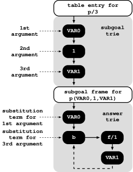
Figure 5: Table space organization

An example for a tabled predicate $p/3$ is shown in Fig. 5. Initially, the table entry for $p/3$ points to an empty subgoal trie. Then, the subgoal $p(X,1,Y)$ is called and three trie nodes are inserted to represent the arguments in the call: one for variable $X$ ($VAR_{0}$), a second for integer 1, and a last one for variable $Y$ ($VAR_{1}$). Since the predicate’s functor term is already represented by its table entry, we can avoid inserting an explicit node for $p/3$ in the subgoal trie. Then, the leaf node is set to point to a subgoal frame, from where the answers for the call will be stored. The example shows two answers for $p(X,1,Y)$: {X=$VAR_{0}$, Y=f($VAR_{1}$)} and {X=$VAR_{0}$, Y=b}. Since both answers have the same substitution term for argument $X$, they share the top node in the answer trie ($VAR_{0}$). For argument $Y$, each answer has a different substitution term and, thus, a different path is used to represent each.

When adding answers, the leaf nodes are chained in a linked list in insertion time order, so that the recovery may happen the same way. In Fig. 5, we can observe that the leaf node for the first answer (node $VAR_{1}$) points (dashed arrow) to the leaf node of the second answer (node $b$). To maintain this list, two fields in the subgoal frame data structure point, respectively, to the first and last answer of this list (for simplicity of illustration, these pointers are not shown in Fig. 5). When consuming answers, a consumer node only needs to keep a pointer to the leaf node of its last loaded answer, and consumes more answers just by following the chain. Answers are loaded by traversing the trie nodes bottom-up (again, for simplicity of illustration, such pointers are not shown in Fig. 5).

4.2 Mode-Directed Tabled Subgoal Calls

In YapTab, mode-directed tabled predicates are compiled by extending the table entry data structure to include a mode array, where the information about the modes is stored. In this mode array, the modes appear in the order in which the arguments are accessed, which can be different from their position in the original declaration. For example, index arguments must be considered first, irrespective of their position. Or, if using the all and min modes in a declaration, all min arguments must be considered before any all argument, since the all means that all answers must be stored, making meaningless the notion of being minimal in this case. As we will see in Section 4.3, changing the order is also strictly necessary to achieve an efficient implementation. In YapTab, the mode information is thus stored in the order mentioned below, together with the argument’s position:

1. arguments with index mode;

2. arguments with max or min mode;

3. arguments with all mode;

4. argument (only one is allowed) with sum or last mode;

5. arguments with first mode.

Figure 6 shows an example for a p(all,index,min) mode-directed tabled predicate. The index mode is placed first in the mode array, then the min mode and last the all mode.

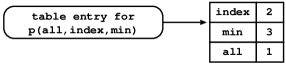
Figure 6: Mode array

During tabled evaluation, new tabled subgoal calls are inserted in their own subgoal tries by following the order of the arguments in the call. With mode-directed tabling, we follow the order defined in the corresponding mode array. For example, consider again the mode-directed tabled predicate p/3 as declared in Fig. 6 and the subgoal call p(X,1,Y). Figure 7 shows the difference between the resulting subgoal tries with and without mode-directed tabling. The values in the mode array indicate that we should start by inserting first the second argument of the subgoal call ($1$), then the third argument ($Y$ or $VAR_{0}$) and last the first argument ($X$ or $VAR_{1}$).

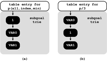
Figure 7: Subgoal tries for p(X,1,Y) considering p/3 declared (a) with and (b) without mode-directed tabling

The mode information is used when creating the subgoal frame associated with the subgoal call at hand. With mode-directed tabling, subgoal frames were extended to include a new array, named substitution array, where the mode information is stored, together with the number of free variables associated with each argument in the subgoal call. The argument’s order is the same as in the mode array.

Figure 8 shows the substitution array for the subgoal call p(X,1,Y). The first position, corresponding to the argument with the constant 1, has no free variables and thus we store a 0 in the substitution array. The other two arguments are free variables and, thus, they have a 1 in the substitution array. It is possible to optimize the array by removing entries that have 0 variables and by joining contiguous entries with the same mode. As we will see next, the substitution array plays an important role in the process of inserting answers in the answer trie.

Figure 8: Substitution array

4.3 Mode-Directed Tabled Answers

Like in traditional tabling, tabled answers are only represented by the substitution terms for the free variables in the arguments of the corresponding subgoal call. However, for mode-directed tabling, when we are considering the substitution terms individually, it is important to know beforehand which mode applies to each, and for that, we use the information stored in the corresponding substitution array. Moreover, the substitutions must be considered in the same order that the variables they substitute have been inserted in the subgoal trie.

Consider again the substitution array for the subgoal call p(X,1,Y). Now, if we find the answer {X=f(a), Y=5}, the first binding to be considered is {Y=5} with min mode and then {X=f(a)} with all mode. Since the answer trie is initially empty, both terms can be inserted as usual. Later, if another answer is found, for example, {X=b, Y=3}, we begin the insertion process by considering the binding {Y=3} with min mode. As there is already an answer in the table, we must compare both accordingly to the min mode. Since the new answer is preferable ($3<5$), the old answer must be invalidated and the new one inserted in the table. The invalidation process consists in: (a) deleting all intermediate nodes corresponding to the answers being invalidated; and (b) tagging the leaf nodes of such answers as invalid nodes. Invalid nodes are only deleted when the table is later completed or abolished. Figure 9 illustrates the aspect of the answer trie before and after the invalidation process.

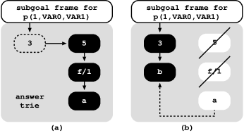
Figure 9: Invalidating answers for p(X,1,Y) (a) before and (b) after the invalidation process

Invalid nodes are opaque to subsequent subgoal calls, but can be still visible from the consumer calls already in evaluation. Hence, when invalidating a node, we may have consumers still pointing to it. By deleting leaf nodes, this would make consumers unable to follow the chain of answers. An alternative would be to traverse the stacks and update the consumers pointing to invalidated answers, but this could be a very costly operation.

Notice also that the mode’s order in the substitution array is crucial for the simplicity and efficiency of the invalidation process. When, at a given node $N$, we decide that an answer should be invalidated, the substitution array’s order ensures that all nodes below node $N$ (including $N$) are the ones we want to invalidate and that the upper nodes are the ones we want to keep. This might not be the case if we used the original order. For example, consider again the call p(X,1,Y) and the answers {X=f(a), Y=5} and {X=b, Y=3}. Figure 10 illustrates the invalidation process of these answers, if using the original declaration.

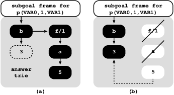
Figure 10: Invalidating answers, without changing the insertion order, for p(X,1,Y) (a) before and (b) after the invalidation process

To detect that the second answer is preferable ($3<5$), we need to navigate in the trie until reaching the leaf node 5 for the first answer. Thus, the invalidation process may require deleting upper nodes (as the example in Fig. 10 shows) and/or traverse several paths to fully detect all preferable answers (this would be the case if we had two intermediate answers with the same minimal values, for instance {X=f(a), Y=5} and {X=h(c), Y=5}), making therefore the invalidation process much more complex and costly.

4.4 Scheduling and Mode-Directed Tabling

In a tabled evaluation, there are several points where we may have to choose between continuing forward execution, backtracking, consuming answers, or completing subgoals. The decision on which operation to perform is determined by the scheduling strategy. The two most successful strategies are batched scheduling and local scheduling [10].

Batched scheduling evaluates programs in a depth-first manner as does the WAM. When new answers are found for a particular tabled subgoal, they are added to the table space and the evaluation continues with forward execution. Only when all clauses have been resolved, the newly found answers will be forwarded to the consumers. Batched scheduling thus tries to delay the need to move around the search tree by batching the consumption of answers.

Local scheduling is an alternative scheduling strategy that tries to complete subgoals as soon as possible. The key idea is that whenever new answers are found, they are added to the table space, as usual, but execution fails. Local scheduling thus explores the whole search space for a tabled predicate before returning answers for forward execution.

To the best of our knowledge, YapTab is the only tabling system that supports the dynamic mixed-strategy evaluation of batched and local scheduling within the same evaluation [11]. This is very important, because for mode-directed tabled predicates, the ability of being able to use local evaluation can be crucial to correctly and/or efficiently support some modes.

$:-~{}table~{}num\_links(index,sum).$
$num\_links(A,0):-~{}edge(\_,A).$
$num\_links(A,1):-~{}edge(A,\_).$

$:-~{}table~{}num\_nodes(sum).$
$num\_nodes(0).$
$num\_nodes(1):-~{}num\_links(\_,\_).$

$edge(a,b).~{}~{}~{}~{}~{}~{}edge(a,c).~{}~{}~{}~{}~{}~{}edge(b,c).$

Figure 11: A cascade of two mode-directed tabled predicates using the sum mode

This is the case for the sum mode. As it sums all the answers for a given argument, we might end with wrong results if we return partial results instead of aggregating them and only returning the aggregated result. Consider, for example, the two mode-directed tabled predicates $num\_links/2$ and $num\_nodes/1$ in Fig. 11 and the query goal $num\_nodes(N)$. If $num\_links/2$ is evaluated using local scheduling, we get the right result (N=3) but, with batched scheduling, we end with a wrong result (N=6). This occurs because, with batched evaluation, the $num\_links(\_,\_)$ call in the second clause of $num\_nodes/2$ succeeds 2 times for each $edge/2$ fact.

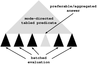
Figure 12: Useless computations with batched evaluation

Batched evaluation can also yield useless computations for mode-directed tabled predicates (see Fig. 12). Consider, for example, a mode-directed tabled predicate $p/1$ declared as $p(max)$ and the query goal:

$:-~{}p(Max),~{}do\_work(Max,Res).$

With batched evaluation, the call to $do\_work(Max,Res)$ will be executed for each $Max$ partial result computed by $p(Max)$, hence originating as many useless computations as the number of non-maximal results.

5 Experimental Results

In this section, we present some experimental results for a set of benchmarks that take advantage of mode-directed tabling. The environment for our experiment was a machine with a AMD FX(tm)-8150 8-core processor with 32 GBytes of main memory and running the Linux kernel 64 bits version 3.2.0. To put our results in perspective, we compare our implementation, on top of Yap Prolog (development version 6.3), with the B-Prolog (version 7.8 beta-6) and the XSB (version 3.3.6) systems, both using local scheduling. For XSB, we adapted the benchmarks to use lattice answer subsumption (as discussed in Section 3.4). For benchmarking, we used the following set of programs:

shortest(N)

uses the min mode to determine all-pairs shortest paths in a graph representing the flight connections between the N busiest commercial airports in US.

shortest_first(N)

uses the first mode to extend the all-pairs shortest paths program to also include the first justification for each shortest path.

shortest_all(N)

uses the all mode to extend the all-pairs shortest paths program to also include all the justifications for each shortest path.

shortest_pref(N)

uses the last mode to solve the all-pairs shortest paths program using Preferences [8].

knapsack(N)

uses the max mode to determine the maximum number of items to include in a collection, from N weighted items, so that the total weight is equal to a given value.

lcs(N)

uses the max mode to find the longest subsequence common to two different sequences of size N.

matrix(N)

uses the min mode to implement the matrix chain multiplication problem that determines the most efficient way to multiply a sequence of N matrices.

pagerank(N)

uses the sum mode to measure the rank values of web pages in a realistic dataset of web links called search engines, using N iterations.

Table 1 shows the execution times, in milliseconds, for running the benchmarks with YapTab, B-Prolog and XSB. In parentheses, it also shows the overhead ratios against YapTab with local evaluation. The execution times are the average of 3 runs. The entries marked with $n.a.$ correspond to programs using modes not available in B-Prolog. The ratios marked with (—) mean that we are not considering them in the average results (they correspond either to $n.a.$ entries or to execution times much higher than YapTab).

Table 1: Execution times, in milliseconds, for YapTab, B-Prolog and XSB and the respective overhead ratios when compared with YapTab’s local evaluation

Programs	YapTab		B-Prolog	XSB
	Local	Batched
shortest(300)	1,088	1,261 (1.16)	2.990 (2.37)	2,922 (2.69)
shortest(400)	1,544	1,785 (1.16)	4,216 (2.36)	4,321 (2.80)
shortest(500)	2,170	2,472 (1.14)	5,792 (2.34)	6,218 (2.87)
shortest_first(300)	1,394	2,641 (1.89)	3,225 (1.22)	5,013 (3.60)
shortest_first(400)	2,052	3,432 (1.67)	4,614 (1.34)	7,257 (3.54)
shortest_first(500)	2,866	4,228 (1.57)	7,400 (1.42)	10,328 (3.60)
shortest_all(300)	4,324	8,383 (1.94)	$n.a.$ (—)	61,803 (—)
shortest_all(400)	5,861	10,590 (1.81)	$n.a.$ (—)	122,985 (—)
shortest_all(500)	8,337	13,598 (1.63)	$n.a.$ (—)	239,451 (—)
shortest_pref(300)	2,882	4,241 (1.47)	$n.a.$ (—)	6,666 (2.31)
shortest_pref(400)	4,152	5,621 (1.35)	$n.a.$ (—)	9,932 (2.39)
shortest_pref(500)	5,773	7,473 (1.29)	$n.a.$ (—)	14,129 (2.45)
knapsack(1000)	1,013	998 (0.99)	837 (0.84)	2,684 (2.65)
knapsack(1500)	1,581	1,561 (0.99)	1,229 (0.79)	3,977 (2.52)
knapsack(2000)	2,037	2,040 (1.00)	1,582 (0.78)	5,473 (2.69)
lcs(1000)	1,196	1,416 (0.98)	2,900 (2.48)	3,060 (2.56)
lcs(1500)	2,768	3,560 (0.98)	5,784 (2.12)	7,128 (2.58)
lcs(2000)	4,864	6,053 (0.99)	10,116 (2.11)	13,338 (2.74)
matrix(100)	192	224 (1.17)	582 (2.60)	396 (2.06)
matrix(150)	925	1,076 (1.16)	2,549 (2.37)	1,610 (1.74)
matrix(200)	3,005	3,534 (1.18)	7,816 (2.21)	4,688 (1.56)
pagerank(1)	365	$n.a.$ (—)	$n.a.$ (—)	128,377 (—)
pagerank(16)	813	$n.a.$ (—)	$n.a.$ (—)	$>10~{}min$ (—)
pagerank(36)	1,260	$n.a.$ (—)	$n.a.$ (—)	$>10~{}min$ (—)
Average		(1.29)	(1.82)	(2.49)

In general, the results show that, for all combinations of experiments and systems, there is no clear tendency showing that the overhead ratios increase or decrease as we increase the size of the corresponding set of programs.

Comparing the results for local and batched evaluation, they show that, on average, batched evaluation is around 29% worse than local evaluation. Batched evaluation gets worse the more answers are inserted into the table space. This affects in particular the shortest_first(), shortest_all() and shortest_pref() set of programs, which confirms our discussion regarding the fact that batched evaluation is more suitable to useless computations.

Regarding the comparison with the other systems, the results obtained for YapTab clearly outperform those of B-Prolog and XSB. On average, B-Prolog and XSB are, respectively, around 1.82 and 2.49 times worse than YapTab using local evaluation.

Please note that for B-Prolog and XSB we do not include the performance of some programs into the average results. For B-Prolog, this is because these programs use the all, last and sum modes, which are not supported in B-Prolog. For XSB, the execution times for the shortest_all() and pagerank() are much higher than YapTab and including them would have distorted the comparison between the three systems. To the best of our knowledge, YapTab is thus the only system that supports the all, last and sum modes and handles them efficiently.

6 Conclusions

We discussed how we have extended and optimized YapTab’s table space organization to provide engine support for mode-directed tabling. In particular, we presented how we deal with mode-directed tabled subgoal calls and answers and we discussed the role of scheduling in mode-directed tabled evaluations. Our implementation uses a more general approach to the declaration and use of mode operators and, currently, it supports 7 different modes. To the best of our knowledge, no other tabling system supports all these modes and, in particular, the sum mode is not supported by any other system. Experimental results on benchmarks that take advantage of mode-directed tabling, showed that our implementation clearly outperforms the B-Prolog and XSB state-of-the-art Prolog tabling systems. In particular, YapTab is the only system that efficiently handles programs that use the all mode. Further work will include extending our implementation to support multi-threaded mode-directed tabling.

References

- [1] Chen, W., Warren, D.S.: Tabled Evaluation with Delaying for General Logic Programs. Journal of the ACM 43(1) (1996) 20–74
- [2] Guo, H.F., Gupta, G.: Simplifying Dynamic Programming via Mode-directed Tabling. Software Practice and Experience 38(1) (2008) 75–94
- [3] Zhou, N.F., Kameya, Y., Sato, T.: Mode-Directed Tabling for Dynamic Programming, Machine Learning, and Constraint Solving. In: IEEE International Conference on Tools with Artificial Intelligence. Volume 2., IEEE Computer Society (2010) 213–218
- [4] Swift, T., Warren, D.S.: Tabling with Answer Subsumption: Implementation, Applications and Performance. In: European Conference on Logics in Artificial Intelligence. Number 6341 in LNAI, Springer-Verlag (2010) 300–312
- [5] Rocha, R., Silva, F., Santos Costa, V.: On applying or-parallelism and tabling to logic programs. Theory and Practice of Logic Programming 5(1 & 2) (2005) 161–205
- [6] Ramakrishnan, I.V., Rao, P., Sagonas, K., Swift, T., Warren, D.S.: Efficient Access Mechanisms for Tabled Logic Programs. Journal of Logic Programming 38(1) (1999) 31–54
- [7] Guo, H.F., Jayaraman, B., Gupta, G., Liu, M.: Optimization with Mode-Directed Preferences. In: 7th ACM SIGPLAN International Conference on Principles and Practice of Declarative Programming, ACM (2005) 242–251
- [8] Santos, J., Rocha, R.: Mode-Directed Tabling and Applications in the YapTab System. In: Symposium on Languages, Applications and Technologies. (2012) 25–40
- [9] Bachmair, L., Chen, T., Ramakrishnan, I.V.: Associative Commutative Discrimination Nets. In: International Joint Conference on Theory and Practice of Software Development. Number 668 in LNCS, Springer-Verlag (1993) 61–74
- [10] Freire, J., Swift, T., Warren, D.S.: Beyond Depth-First: Improving Tabled Logic Programs through Alternative Scheduling Strategies. In: International Symposium on Programming Language Implementation and Logic Programming. Number 1140 in LNCS, Springer-Verlag (1996) 243–258
- [11] Rocha, R., Silva, F., Santos Costa, V.: Dynamic Mixed-Strategy Evaluation of Tabled Logic Programs. In: International Conference on Logic Programming. Number 3668 in LNCS, Springer-Verlag (2005) 250–264