∎
Mean-field analysis of the -voter model on networks
Abstract
We present a detailed investigation of the behavior of the nonlinear -voter model for opinion dynamics. At the mean-field level we derive analytically, for any value of the number of agents involved in the elementary update, the phase diagram, the exit probability and the consensus time at the transition point. The mean-field formalism is extended to the case that the interaction pattern is given by generic heterogeneous networks. We finally discuss the case of random regular networks and compare analytical results with simulations.
Keywords:
social dynamics opinion dynamics voter model1 Introduction
Ordering dynamics is a classical subject of nonequilibrium statistical physics, regarding phenomena such as magnetic ordering or phase-separation of mixtures Bray94 ; KineticViewRedner . Also in the biological and social domains the question of how order emerges and evolves over time is of fundamental interest. This has recently led to the introduction of a wealth of models for ordering dynamics in interdisciplinary settings, inspired by the physical paradigms but exhibiting a diversity of specific distinctive features Castellano09 . In this context the voter model Clifford73 ; Holley:1975fk plays a prominent role for several reasons: it is extremely simple; it has a natural interpretation in several fields (ecology, genetics, opinion dynamics); it can be exactly solved in regular lattices for any number of spatial dimensions liggett99:_stoch_inter ; KineticViewRedner .
The voter model is defined as follows: A population of agents is placed on a regular lattice or a graph of size . Each agent is endowed with a binary spin variable, representing two opposed opinions, and taking values . At each time step , an agent , together with one nearest neighbor , are selected at random, and the state of the system is updated as , the first agent copying the opinion of its neighbor. Time is updated . In this way, the flipping probability, i.e. the probability that a spin surrounded by a fraction of spins in the opposite state flips, is . Starting from a disordered initial state, this dynamics leads in finite systems to a uniform state with all individuals sharing the same opinion (the so-called consensus). From the social dynamics point of view, interest is mainly focused on the exit probability and the consensus time , defined as the probability that the final state corresponds to all agents in the state and the average time needed to reach consensus in a system of size , respectively, when starting from a homogeneous initial condition with a fraction of agents in state Castellano09 . On regular lattices voter dynamics conserves on average the global magnetization , and this implies . On the other hand, for 1751-8121-43-38-385003 the consensus time takes the form
| (1) |
with in , in , and in (the latter being also the mean-field result) KineticViewRedner .
In the social context voter dynamics becomes all the more relevant when it is considered on top of complex networks, which are more realistic representations of social contact or relationship patterns barabasi02 ; Newman2010 . The analysis on these substrates reveals nontrivial differences with respect to lattices. For example, now the order in which interacting individuals are selected matters Suchecki05 ; castellano05:_effec . Moreover, relevant quantities such as the exit probability and the consensus time turn out to depend on the heterogeneity of the contact pattern, as measured by the degree distribution PhysRevLett.94.178701 ; Sood08 ; Pugliese09 . On complex networks the main conserved quantity is not the total magnetization, but a connectivity weighted magnetization, . Thus, it is possible to show that the exit probability is equal to this conserved quantity, while the consensus time takes the form PhysRevLett.94.178701
| (2) |
where now , with the -th moment of the degree distribution.
In the case of regular lattices, the simple behavior of the voter model has been shown to be more generic than its original definition apparently shows. Early work showed that the voter model lies at a transition point between a ferromagnetic ordered phase and a paramagnetic disordered phase, such that any small perturbation is able to drive it out of the transition and radically change its behavior Deoliveira93 ; Drouffe99 ; Molofsky99 . Further work on this issue, based on numerical simulations and phenomenological field theories has finally led to the realization that there exists a whole generalized voter (GV) universality class encompassing models at an order-disorder transition driven by interfacial noise between “dynamically equivalent” absorbing states. The equivalence can be enforced either by -symmetric local rules, or by global conservation of the magnetization Dornic01 ; AlHammal05 . The newly observed GV universality class is defined in terms of the critical exponents characterizing the transition. However, recent research has shown that other characteristics, such as the shapes of the exit probability and the consensus times, exhibit nonuniversal features, depending on the microscopic details defining the model Castellano12 .
The investigation of the existence and the properties of the GV class is based on the consideration of nonlinear voter models, in which the flipping probability is a function taking a nonlinear form Dornic01 ; Vazquez08 . In the general case, the nonlinearity of the flipping probability can be considered to be modulated by a tunable parameter and the GV behavior occurs for a critical value , that separates a ferromagnetic (ordered) phase, in which the systems orders with a time that scales logarithmically with the system size, from a paramagnetic (disordered) phase, in which the systems orders at exponentially large times. Few exact results are available about these models, since contrary to the standard voter model, nonlinear voter models are not in general analytically solvable. Therefore, our understanding of the GV class is mainly based on numerical simulations and on the analysis of field theories, which are studied also numerically or by means of renormalization group arguments Canet05 . In this sense, analytical results for nonlinear voter models can in general be produced only at the mean field level.
In this paper we focus in the analysis of the mean field behavior on networks of a nonlinear voter model recently introduced in the context of opinion dynamics the -voter model PhysRevE.80.041129 . This model is characterized by two parameters, representing the number of interacting voters , and a source of noise . A critical value of the parameter identifies the GV transition, taking a functional form depending on the particular value of . Considering initially the simplest case of a fully connected graph, we solve the Fokker-Planck equation that represents the dynamics, and obtain analytical information for different values of . We show that, even in the simplest mean-field case, nonlinear voter models can show a very rich behavior, characterized by a complex phase diagram for sufficiently large values of . We then introduce a theoretical treatment, within the heterogeneous mean-field framework, for the -voter dynamics on generic uncorrelated networks. We finally turn to the consideration of random regular networks as substrate of the dynamics.
2 The -voter model
On an arbitrary lattice or graph, the -voter model is defined as follows: Each node hosts a spin, with a binary value . The system evolves dynamically by selecting, at a given time , a randomly chosen spin located at, say, node , with state . Additionally, neighbors of node are also chosen at random, allowing for repetition. If all the neighbors are in the same state, , the original spin takes the value of the neighbors, ; otherwise, and with an independent probability .the original spin flips its state, . In any case, time is updated , where is the total number of sites.
It is easy to see that this model is non-linear. Consider the probability that a site flips as a function of the fraction of neighbors in the opposite state. The flipping probability can be easily seen to take the form
| (3) |
For , we recover, for any value of , the standard voter model, namely . For , on the other hand, the flipping probability takes the form
| (4) |
For , , and therefore linear voter behavior must be observed for this combination of parameters in any kind of substrate. In order to observe truly nonlinear behavior in the -voter model (in the sense that at the transition), we must thus consider values of larger than .
3 The -voter model on fully connected graphs
The case of a fully connected graph corresponds to the classic mean-field behavior, in which every node is neighbor of all the other nodes in the system. Therefore, choosing neighbors at random corresponds to the random selection of any nodes in the system. In this case, the state of the system is fully characterized by number of sites in state . The behavior of the -voter model can be derived in this regime by means of the exact diffusion formalism developed in Ref. 1751-8121-43-38-385003 . Here we follow however a more intuitive approach based on the Fokker-Planck equation Gardinerbook ; blythe07:_stoch_model . The probability of finding the systems in state at time fulfills the master equation
| (5) |
where are the transition rates from a state with to a state with positive spins. The only non-zero transition rates can be seen to take the form, for a fully connected graph,
| (6) | |||||
| (7) | |||||
| (8) |
where is the elementary time scale of the problem and we have defined . Performing an expansion up to second order in , the previous master equation can be converted into a simplified Fokker-Planck equation, valid in the limit of large system sizes, taking the form
| (9) |
where we have defined the drift and the diffusion coefficients , taking the forms
| (10) | |||||
| (11) |
From the Fokker-Planck equation, application of a standard formalism Gardinerbook leads to an exit probability satisfying the differential equation
| (12) |
with boundary conditions and , while the average time until consensus, , is given by
| (13) |
with boundary conditions .
Linear flipping probability implies absence of drift, and then linear exit probability . Moreover, it is easy to see from Eqs. (1) and (13), that a zero drift is necessary and sufficient condition to yield, for any diffusion scaling as , and , which are the two main signatures of voter behavior at the mean-field level. Let us consider what is the behavior of the -voter model for different values of .
3.1 Case
For , the drift and the diffusion coefficient take the form
| (14) | |||||
| (15) |
The value leads to linear voter behavior, with . On the other hand, the drift takes the form , leading to a consensus time of the form
| (16) |
which coincides with the form observed in regular lattices for dimension , Eq. (1). From Eq. (14), we can easily see that implies for and for , which is indicative of a ferromagnetic ordered state. The opposite behavior is found for , indicating a disordered paramagnetic phase. Therefore, the point , corresponding to linear voter behavior, lies at a transition between a ferromagnetic and a paramagnetic phase.
3.2 Case
In the case , we have
| (17) | |||||
| (18) |
The value separates again a ferromagnetic phase at from a paramagnetic phase for . Exactly at , we recover , which leads to a linear exit probability, but now . The diffusion term is now different from the case of the linear voter, and as a consequence it will lead to a different form of the consensus time as a function of . The form can be recovered by integrating Eq. (13), upon substituting the diffusion in Eq. (18), namely
| (19) |
The integration of this differential equation takes the form
| (20) | |||||
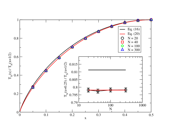
In Fig. 1 we plot the normalized consensus time for the -voter model and , Eq. (20), compared with the result from the linear voter model, Eq. (16). The difference induced by the nonlinear form of is small but noticeable, and indeed it is recovered by means of numerical simulations on a fully connected graph (symbols in Fig. 1).
3.3 Case
In the more interesting case of , the drift and diffusion coefficient take the forms
| (21) | |||||
| (22) |
From this form of the drift, it is easy to check that there exists no value of that allows it to vanish for every value of . Therefore, there is no region of linear voter behavior in the phase diagram of this model. In order to visualize the form of this phase diagram, it is convenient to change variables and represent the drift as a function of the average magnetization . With this transformation, the drift takes the form
| (23) |
A ferromagnetic phase will correspond to the region of values of for which for all , while a paramagnetic phase corresponds to . From Eq. (23), we can see that the nature of the phase is given by the sign of the function
| (24) |
The ferromagnetic phase corresponds to , which takes place in the region ; the region corresponds to a paramagnetic phase with ; on the other hand, the region is a mixed phase, which is ferromagnetic or paramagnetic depending on the initial value of . In particular, initial conditions with magnetization lead to a paramagnetic behavior, while corresponds to a ferromagnetic phase.
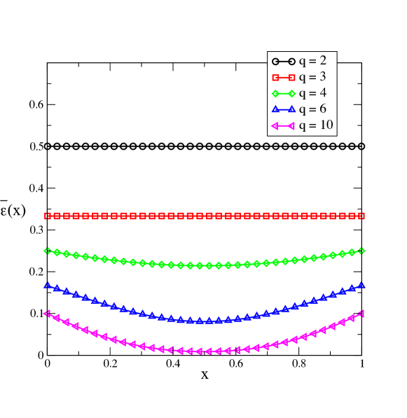
The ensuing phase diagram for the -voter model on fully connected graphs is depicted, as a function of the density of spins, in Fig. 2.
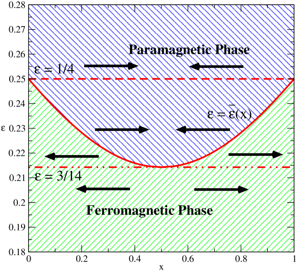
Summarizing its structure, for , there is a paramagnetic disordered phase, with growing exponentially with and in the limit of large . For , on the other hand, a ferromagnetic phase appears, with a fast consensus time scaling logarithmically with system size, and an exit probability tending to a step-function. Finally, in the region there is a mixed phase such that for , we should expect a paramagnetic disordered phase, while for , the system should order to consensus given by the majority of initial spins. The boundary separating both behaviors in the mixed phase is given by an effective as
| (25) |
such that for , a paramagnetic phase is observed, while corresponds to the ferromagnetic phase.
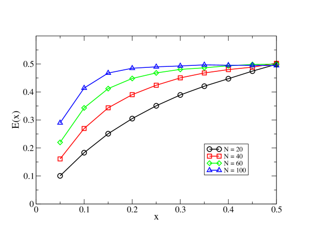
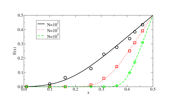
In Fig. 3 we check the predicted behavior in fully connected networks by measuring numerically the exit probability for increasing system size and three values of representing the three phases discussed above. For , tends to , independent of , as expected in the paramagnetic phase. For instead the tendency is toward a step-function , indicating a ferromagnetic phase. In the intermediate regime () the ferromagnetic phase dominates for and , while the region around is paramagnetic.
In analogy with the GV class, one should expect to observe nontrivial behavior in the separatrix between the paramagnetic and the ferromagnetic phase. In the case of the -voter model, this separatrix, is not a constant, and therefore it is impossible to study its behavior in the general case. We shall therefore focus on the minimum of the separatrix, given by the points , and . Considering Eq. (13), and changing again to the total magnetization variable , we are led for to the equation for the consensus time
| (26) |
with boundary conditions reading now , and where
| (27) | |||||
| (28) |
By defining
| (29) |
the exact solution to Eq. (26) is given in integral form by
| (30) |
We notice that since the first exponential is peaked around as , it will select values of in the second integral, which can be thus expanded for small . An estimate of the consensus time can thus be expressed in terms of error functions abramovitz as follows
| (31) | |||||
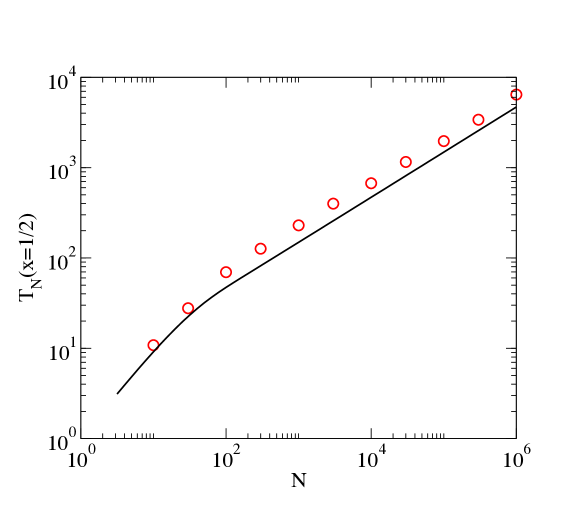
At the point (), the consensus time takes the form
| (32) |
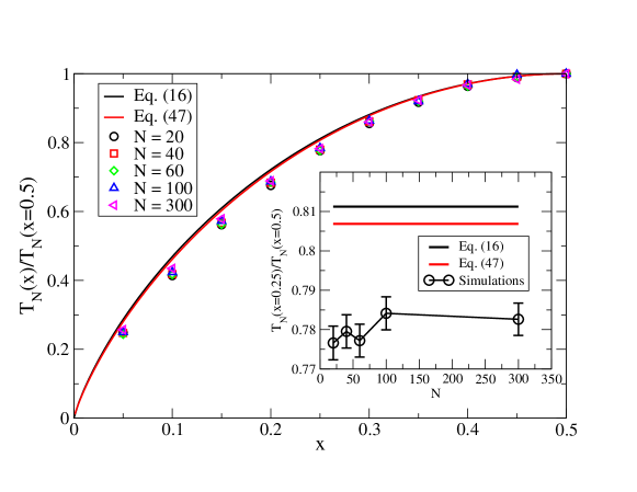
This expression recovers the observed scaling in the large limit PhysRevE.80.041129 , and is found in good agreement with numerical simulation results, as shown in Fig. 4.
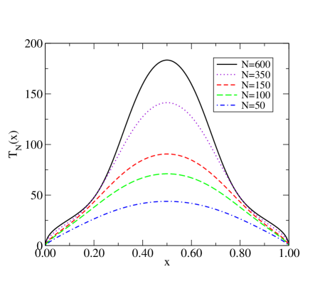
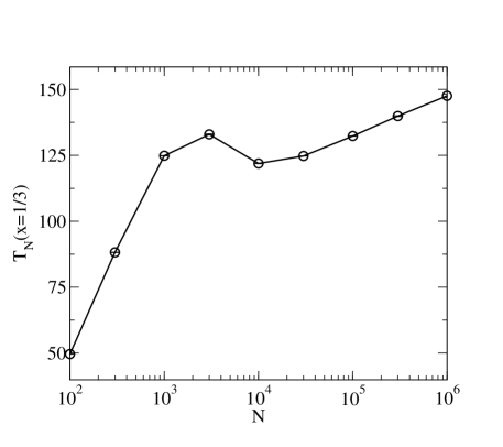
For the system is in the ferromagnetic phase and one expects the consensus time to scale logarithmically for large values of the system size . By direct numerical integration of Eq. (30), the value of the consensus time for any value of and can be computed, see Fig. 5 (left panel). The crossover between the behavior at , , and the pure logarithmic growth which asymptotically prevails for all , give rise to a nonmonotonicity in the functional form of as a function of , see Fig. 5 (right panel). This is a curious phenomenon: there is a short range of values of for which the consensus time decreases as is increased.
Concerning the exit probability, the solution of the corresponding equation leads to the form, again expressed in terms of the magnetization ,
| (33) |
Expanding the integral in powers of , and keeping only the first order, we are led to
| (34) |
Focusing on the case (), due to the symmetry of the expression, the integral can be performed, yielding
| (35) |
where is the Gamma function and is the incomplete Gamma function abramovitz . In Fig. 6 we plot Eq. (35) together with numerical simulations, displaying again a good agreement for values of larger than .
3.4 Phase diagram for general
Following the same arguments as in the previous section, we can sketch a phase diagram for the general case of the -voter model by considering the sign of the function . Considering the form of the drift in Eq. (10) and the flipping probability in Eq. (3), simple calculations allow to show that the quantity is positive for , with taking the form (expressed as a function of for simplicity)
| (36) |
In Fig. 7 we plot the shape of the phase boundary , Eq. (36), as a function of , for different values of .
We observe that
| (37) |
We thus obtain that, for the general case, the -voter model is in a ferromagnetic phase for , and in a paramagnetic phase for . In the region , the system is in a mixed phase whose nature depends on the initial conditions. In the limit of large , the boundary of region for ferromagnetic behavior decreases exponentially, while the boundary for paramagnetic behavior decreases only algebraically.
4 The -voter model on networks: General heterogeneous mean-field theory
The analytical treatment of voter-like models on complex networks, beyond the simplest fully connected graph, is traditionally based on the heterogeneous mean-field (HMF) approach, a powerful tool for the theoretical analysis of general dynamical processes on heterogeneous substrates barratbook ; dorogovtsev07:_critic_phenom . HMF theory is based on a fundamental approximation: The real (quenched) network is coarse-grained into an annealed one dorogovtsev07:_critic_phenom , which disregards the specific connection pattern and postulates that the class of degree is connected to the class of degree with conditional probability marian1 .
The application of the HMF formalism to the -voter model follows from an extension of the case of standard voter model PhysRevLett.94.178701 ; Sood08 , taking into account the intrinsic multipoint nature of the -voter dynamical rules. Indeed, the annealed network approximation is based on the assumption that the network gets completely rewired between any two dynamical time steps. In dynamics in which a vertex interacts with a single neighbor, or with all of them, the numerical (and analytical) implementation goes by selecting one or (according to the case) neighbors, randomly chosen with probability , where we are for simplicity making the further assumption that the network lacks degree correlations, i.e. Dorogovtsev:2002 .
In the -voter model, we choose neighbors, possibly with repetition, among the neighbors of a vertex. If we choose these neighbors at random among all the vertices in the network, we are implicitly assuming that there is rewiring of the network even during the duration of an elementary dynamic step and this underestimates the probability that repetitions occur, i.e. a neighbor is selected multiple times. The proper way to eliminate this inconsistency is to select at random a fixed set of neighbors among all the vertices in the network, and then to pick up the participants to the dynamic step only from the fixed set of neighbors previously selected.
Let us thus consider a generic sparse network. Assuming no correlations and annealed approximation, the probability that a randomly chosen neighbor of a vertex is in state is given by
| (38) |
where is the probability that a vertex of degree is in state . In the set of neighbors of a vertex of degree , chosen to make an elementary update of this vertex, the probability that we choose in state is given by the binomial distribution . In this case, if vertex is in state , it will flip with probability
| (39) |
while if it is in state , it will flip with probability . Therefore, the probabilities that a microscopic update will flip a spin of degree and state morettiheterovoter are given by the elementary flipping probabilities, and , averaged over the binomial distribution , and take the form
| (40) | |||||
| (41) |
where the first terms stand for the probability of selecting a vertex to update of degree , , and the probability that it is in state (), or (), respectively. The HMF equation for the time evolution of the density takes the form
| (42) |
From this solution, one can find information about the exit probability by looking for conservation laws of the dynamics in Eq. (42), while the consensus time follows from an immediate one-step calculation complemented with an adiabatic approximation, which allows to replace the multiple degrees of freedom by single slowly varying conserved quantity PhysRevLett.94.178701 ; Sood08 .
For and any network, the application of this formalism leads to the trivial result presented in Sec. 2. For values of , the application of this formalism is hampered by the fact that the (possible) conserved quantities in Eq. (42) are not linear functions of , which implies that the transformations leading to the equation for the consensus time cannot be applied directly morettiheterovoter . We therefore consider in the following section the simpler case of random regular networks, where a full analytical solution can be obtained for .
5 The -voter model on random regular networks
Random regular networks (RRN) are networks where all nodes have exactly the same degree , while links are randomly distributed among them, avoiding self-connections and multiple connections. In this case, we have , where is the average (constant) degree of the network. In this particular network, since all vertices share the same value of the degree, a great simplification arises, as we can set , the total average density of vertices in state . Additionally, since the density is homogeneous, we can sidestep the general formalism from HMF theory and apply directly the Fokker-Planck approach presented in Sec. 3.
In the case , the general considerations from Sec. 4 indicate the presence of linear voter behavior for .
5.1 Case
In the more interesting case of , we are led, from Eq. (39), (10), and (11), to a drift and a diffusion coefficient of the form
| (43) | |||||
| (44) |
The drift turns out now to vanish for a value that depends on as
| (45) |
This value tends to , corresponding to a fully connected network, in the limit , but is always larger than for any finite . This observation indicates that the structure of a RRN induces more order than a fully connected topology, and thus that a larger disordering parameter is needed to cross over to the disordered paramagnetic phase.
For this critical value the diffusion coefficient is
Using Eq. (13) we are led to the equation for the consensus time
| (46) |
where , whose solution is
| (47) | |||||
Again, we obtain a non-entropic form, modulated by the factor , and that yields the mean-field result Eq. (20) in the limit ().
To check the above results we have simulated the -voter model on RRN with . In this case, HMF theory predicts a transition at
| (48) |
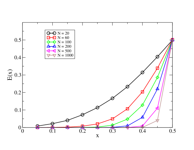
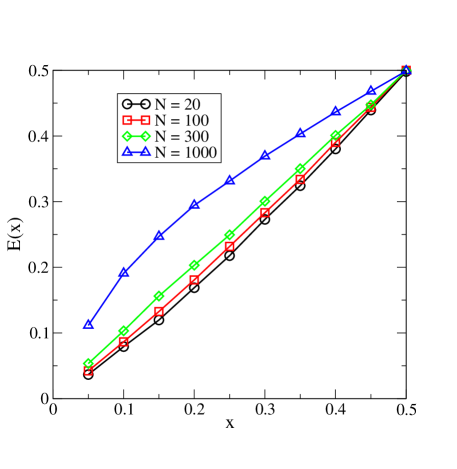
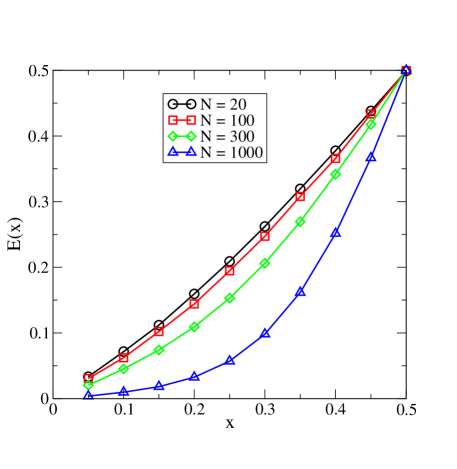
Numerical results lead however at a different, much lower, value. In order to estimate numerically the value of we have followed the following approach, based on the behavior of the exit probability Castellano12 . Indeed, corresponds to a disordered paramagnetic phase with, for asymptotically large systems, , while corresponds to an ordered ferromagnetic phase, where , the Heaviside theta function. Therefore, focusing on an initial density , we should observe for , for , and for when increasing the system size . In Fig. 8 we report the exit probability for and different values of as a function of the lattice size . A plateau is obtained for , while larger (smaller) values of lead to an increase (decrease) of with . We conclude that the critical point is in this case located at , where the error bars are obtained from the values of leading to an increasing or decreasing behavior for .
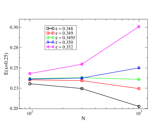
Fig. 8 also indicates that , i.e. the global form of the exit probability at the transition is not linear, in agreement with the findings in Castellano12 . Not unexpectedly, also the dependence of the consensus time on (Fig. 9) turns out to be different from the analytical prediction, Eq. (47)).
5.2 Case
The case of in RRN leads to rather complex expressions. In particular, as a function of the magnetization , the drift takes the form
| (49) |
As in the case of the fully-connected graph, no value of can make this expression zero for any . Therefore we exclude again for this value of the presence of a linear voter point. Performing a similar analysis as in Sec. 3.3, we can however determine the phase diagram by looking at the sign of the function . It turns out that is positive for smaller than the threshold , which, as a function of , takes the form
| (50) |
The phase-diagram is perfectly analogous to the one illustrated in Fig. 2, with a ferromagnetic phase for
| (51) |
a paramagnetic phase for
| (52) |
and an intermediate mixed phase, whose nature depends on the initial condition .
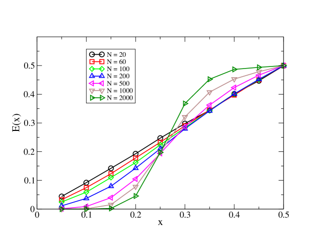
The interesting question is whether the real -voter dynamics in quenched RRN networks obeys (at least qualitatively) these theoretical predictions, in particular with respect to the existence of the mixed phase. We have checked this by means of numerical simulations in RRN with . In this case, Eq. (50) predicts a mixed phase for values of in the range . Numerically we observe instead (Fig. 10) that there is a simple transition (for ) separating a purely ferromagnetic phase for (where tends to a step-function ), from a purely paramagnetic phase for (where tends to for any ). Hence we conclude that the fluctuations introduced by the RRN quenched topology are sufficient to make the behavior of the -voter model similar to what happens on finite-dimensional lattices PhysRevE.80.041129 ; Castellano12 and qualitatively different from what happens on fully-connected graphs. We expect similar conclusions to hold for any and for any .
6 Conclusions
In this paper we have presented a detailed mean-field analysis of a model for social dynamics belonging to the generalized voter universality class. A rich phenomenology emerges, in particular for , with a mixed phase separating paramagnetic and ferromagnetic regions of the phase diagram. When the dynamics occurs on networks a natural question arising is whether the behavior is of mean-field finite dimensional type. From the analysis of random regular networks it turns out that the minimal disorder present in those graphs is sufficient to destroy the mixed phase for and restore a behavior qualitatively similar to what happens in lattices, with a single transition point separating ordered and disordered regions of the phase diagram. Also in the case , the dynamics on RRN is more akin to finite dimensional lattices (nonlinear exit probability at the transition) than complete graphs (where ). Questions about the behavior on complex, heterogeneous networks remain open. In that case it is possible that more interesting phenomena could arise, due to the interplay between the value of and the degree , which has large fluctuations from node to node.
Acknowledgments
R.P.-S. acknowledges financial support from the Spanish MEC, under project No. FIS2010-21781-C02-01; the Junta de Andalucía, under project No. P09-FQM4682; ICREA Academia, funded by the Generalitat de Catalunya; partial support by the NSF under Grant No. PHY1066293, and the hospitality of the Aspen Center for Physics, CO, USA, where part of this work was performed. P.M acknowledges financial support from Junta de Andalucía project P09-FQM4682 and MICINN–FEDER project FIS2009–08451. S.Y.L acknowledges the support of the 973 Program of China (No.2012CB720500) and the National High Technology R&D Program of China (2012AA041102).
References
- (1) Abramowitz, M., Stegun, I.A.: Handbook of mathematical functions. Dover, New York (1972)
- (2) Al Hammal, O., Chaté, H., Dornic, I., Mu ̃noz, M.A.: Langevin description of critical phenomena with two symmetric a bsorbing states. Phys. Rev. Lett. 94, 230601 (2005)
- (3) Albert, R., Barabási, A.L.: Statistical mechanics of complex networks. Rev. Mod. Phys. 74, 47–97 (2002)
- (4) Barrat, A., Barthélemy, M., Vespignani, A.: Dynamical Processes on Complex Networks. Cambridge University Press, Cambridge (2008)
- (5) Blythe, R.A.: Ordering in voter models on networks: exact reduction to a single-coordinate diffusion. J. Phys. A 43, 385003 (2010)
- (6) Blythe, R.A., McKane, A.J.: Stochastic models of evolution in genetics, ecology and linguistics. J. Stat. Mech. p. P07018 (2007)
- (7) Boguñá, M., Pastor-Satorras, R.: Epidemic spreading in correlated complex networks. Phys. Rev. E 66, 047104 (2002)
- (8) Bray, A.J.: Theory of phase-ordering kinetics. Adv. Phys. 43, 357–459 (1994)
- (9) Canet, L., Chaté, H., Delamotte, B., Dornic, I., Muñoz, M.A.: Nonperturbative fixed point in a nonequilibrium phase transition. Phys. Rev. Lett. 95, 100601 (2005)
- (10) Castellano, C.: Effect of network topology on the ordering dynamics of voter models. AIP Conf. Proc. 779, 114 (2005)
- (11) Castellano, C., Fortunato, S., Loreto, V.: Statistical physics of social dynamics. Rev. Mod. Phys. 81, 591–646 (2009)
- (12) Castellano, C., Muñoz, M.A., Pastor-Satorras, R.: Nonlinear -voter model. Phys. Rev. E 80, 041129 (2009)
- (13) Castellano, C., Pastor-Satorras, R.: Universal and nonuniversal features of the generalized voter class for ordering dynamics in two dimensions. Phys. Rev. E 86, 051123 (2012)
- (14) Clifford, P., Sudbury, A.: A model for spatial conflict. Biometrika 60, 581–588 (1973)
- (15) Dornic, I., Chaté, H., Chave, J., Hin richsen, H.: Critical coarsening without surface tension: The universality class of the voter model. Phys. Rev. Lett. 87, 045701 (2001)
- (16) Dorogovtsev, S.N., Goltsev, A.V., Mendes, J.F.F.: Critical phenomena in complex networks. Rev. Mod. Phys. 80, 1275–1335 (2008)
- (17) Dorogovtsev, S.N., Mendes, J.F.F.: Evolution of networks. Adv. Phy. 51, 1079–1187 (2002)
- (18) Drouffe, J.M., Godrèche, C.: Phase ordering and persistence in a class of stochastic processes interpolating between the Ising and voter models. J. Phys. A 32, 249–261 (1999)
- (19) Gardiner, C.W.: Handbook of stochastic methods, 2nd edn. Springer, Berlin (1985)
- (20) Holley, R.A., Liggett, T.M.: Ergodic theorems for weakly interacting infinite systems and voter model. Annals of Probability 3, 643–663 (1975)
- (21) Krapivsky, P., Redner, S., Ben-Naim, E.: A Kinetic View of Statistical Physics. Cambridge University Press, Cambridge (2010)
- (22) Liggett, T.M.: Stochastic interacting particle systems: Contact, Voter, and Exclusion processes. Springer-Verlag, New York (1999)
- (23) Molofsky, J., Durrett, R., Dushoff, J., Griffeath, D., Levin, S.: Local frequency dependence and global coexistence. Theoretical Population Biology 55, 270 – 282 (1999)
- (24) Moretti, P., Liu, S.Y., Baronchelli, A., Pastor-Satorras, R.: Heterogenous mean-field analysis of a generalized voter-like model on networks. Eur. Phys. J. B 85, 88 (2012)
- (25) Newman, M.E.J.: Networks: An introduction. Oxford University Press, Oxford (2010)
- (26) de Oliveira, M., Mendes, J., Santos, M.: Nonequilibrium spin models with ising universal behaviour. J. Phys. A 26, 2317–2324 (1993)
- (27) Pugliese, E., Castellano, C.: Heterogeneous pair approximation for voter models on networks. Europhys. Lett. 88, 58004 (2009)
- (28) Sood, V., Antal, T., Redner, S.: Voter models on heterogeneous networks. Phys. Rev. E 77, 041121 (2008)
- (29) Sood, V., Redner, S.: Voter model on heterogeneous graphs. Phys. Rev. Lett. 94, 178701 (2005)
- (30) Suchecki, K., Eguíluz, V.M., Miguel, M.S.: Conservation laws for the voter model in complex networks. Europhys. Lett. 69, 228–234 (2005)
- (31) Vázquez, F., López, C.: Systems with two symmetric absorbing states: Relating the micro scopic dynamics with the macroscopic behavior. Phys. Rev. E 78, 061127 (2008)