An Analysis on Minimum $s{\mathchar 45\relax}t$ Cut Capacity of Random Graphs with Specified Degree Distribution

Abstract

The capacity (or maximum flow) of an unicast network is known to be equal to the minimum $s{\mathchar 45\relax}t$ cut capacity due to the max-flow min-cut theorem. If the topology of a network (or link capacities) is dynamically changing or unknown, it is not so trivial to predict statistical properties on the maximum flow of the network. In this paper, we present a probabilistic analysis for evaluating the accumulate distribution of the minimum $s{\mathchar 45\relax}t$ cut capacity on random graphs. The graph ensemble treated in this paper consists of weighted graphs with arbitrary specified degree distribution. The main contribution of our work is a lower bound for the accumulate distribution of the minimum $s{\mathchar 45\relax}t$ cut capacity. From some computer experiments, it is observed that the lower bound derived here reflects the actual statistical behavior of the minimum $s{\mathchar 45\relax}t$ cut capacity of random graphs with specified degrees.

I Introduction

Rapid growth of information flow over a network such as a backbone network for mobile terminals requires efficient utilization of full potential of the network. In a multicast communication scenario, it is well known that appropriate network coding achieves its multicast capacity. Emergence of the network coding have broaden network design strategies for efficient use of wired and wireless networks [1].

The multicast capacity of a directed graph is closely related to the $s{\mathchar 45\relax}t$ maximum flow, which is equal to the minimum $s{\mathchar 45\relax}t$ cut capacity due to the max-flow min-cut theorem [2]. Furthermore, on a unicast network, the minimum $s{\mathchar 45\relax}t$ cut capacity of the network determines the unicast capacity between the terminals $s$ and $t$. Therefore, it is meaningful to study the minimum $s{\mathchar 45\relax}t$ cut capacity for designing an efficient network.

If the topology of a network is static, the corresponding $s{\mathchar 45\relax}t$ maximum flow of the network can be efficiently evaluated in polynomial time by using Ford-Fulkerson algorithm [2]. However, if the topology of a network and its link capacities are dynamically changing or have stochastic nature, it is not so trivial to predict statistical properties on the maximum flow. For example, in a case of wireless network, the link capacities may fluctuate because of the effect of time-varying fading. Another example is an ad-hoc network whose link connections are stochastically determined.

In order to obtain an insight for statistical properties of the minimum $s{\mathchar 45\relax}t$ cut capacity for such random networks, it is natural to investigate statistical properties of minimum $s{\mathchar 45\relax}t$ cut capacity over a random graph ensemble. Such a result may unveil typical behaviors of the minimum $s{\mathchar 45\relax}t$ cut capacity (or maximum flow) for given parameters of a network such as the number of vertices, edges, probabilistic properties of edge weight and degree distributions.

Several theoretical works on the maximum flow of random graphs (i.e., graph ensembles) have been made. In a context of randomized algorithms, Karger showed a sharp concentration result for maximum flow in the asymptotic regime [3]. Ramamoorthy et al. presented another concentration result. The network coding capacities of weighted random graphs and weighted random geometric graphs concentrate around the expected number of nearest neighbors of the source and the sinks [4]. These concentration results indicate an asymptotic properties of the maximum flow of random networks. Wang et al. shows statistical properties of the maximum flow in an asymptotic setting as well. They discussed the random graphs with Bernoulli distributed weights [5].

In this paper, we will present a lower bound for the accumulate distribution of the minimum $s{\mathchar 45\relax}t$ cut capacity of weighted random graphs with specified degree distribution. The approach presented here is totally different from those used in the conventional works [3][4][5]. The basis of the analysis is the correspondence between the cut space of an undirected graph and a binary LDGM (low-density generator-matrix) code [6]. Based on this correspondence, Yano and Wadayama [7] presented an ensemble analysis for the network reliability problem. Fujii and Wadayama [8] proposed a probabilistic analysis for the global minimum cut capacity over the weighted Erdős-Rényi random graphs. The probability distribution of vertex degrees over Erdős-Rényi random graphs follows the Poisson distribution. However, most of degree distributions of real networks are different from the Poisson distribution [9]. This paper extends the idea in [7] and [8] to weighted random graphs with arbitrary specified degree distribution, which may be applicable to more realistic networks. Moreover, this paper deals with $s{\mathchar 45\relax}t$ cut capacity which is more informative on network capacities instead of the global cut capacity [8].

II Preliminaries

In this section, we first introduce several basic definitions and notation used throughout the paper. Then, an ensemble of weighted undirected graphs treated in this paper is defined.

II-A Notation and definitions

A graph $G\stackrel{{\scriptstyle\triangle}}{{=}}(V,E)$ is a pair of a vertex set $V\stackrel{{\scriptstyle\triangle}}{{=}}\{v_{1},v_{2},\ldots,v_{n}\}$ and an edge set $E\stackrel{{\scriptstyle\triangle}}{{=}}\{e_{1},e_{2},\ldots,e_{m}\}$ where $e_{j}=(u,v),u,v\in V$ is an edge. If $e_{j}=(u,v)$ is not an ordered pair, i.e., $(u,v)=(v,u)$, the graph $G$ is called an undirected graph.

If a function $c:E\rightarrow\mathbb{Z}_{\geq 0}$ is defined for an undirected graph $G\stackrel{{\scriptstyle\triangle}}{{=}}(V,E)$, the triple $(V,E,c)$ is considered as a weighted graph. The function $c$ can be seen as weight for edges. The set $\mathbb{Z}_{\geq 0}$ represents the set of non-negative integers. In our context, the weight function $c$ represents the link capacity for each edge.

Assume that a weighted undirected graph $G\stackrel{{\scriptstyle\triangle}}{{=}}(V,E,c)$ is given. A non-overlapping bi-partition $V=X\cup(V\backslash X)$ is called a cut where $X$ is a non-empty proper subset of $V(X\neq V)$. The set of edges bridging $X$ and $V\backslash X$ is referred to as the cut-set corresponding to the cut $(X,V\backslash X)$, which is denoted by $\partial(X)$ (or equivalently $\partial(V\backslash X)$). The cut weight (i.e., cut capacity) of $X$ is defined as $\omega(X)\stackrel{{\scriptstyle\triangle}}{{=}}\sum_{e\in\partial(X)}c(e).$ If a cut $(X,V\backslash X)$ separates two vertices $s,t\in V(s\neq t)$, the cut $(X,V\backslash X)$ is called an $s{\mathchar 45\relax}t$ cut and the corresponding cut-set is called an $s{\mathchar 45\relax}t$ cut-set. The minimum $s{\mathchar 45\relax}t$ cut is an $s{\mathchar 45\relax}t$ cut whose cut weight is the smallest among all the $s{\mathchar 45\relax}t$ cut-sets.

II-B Random graphs with specified degree distribution

In the following, we will define an ensemble of weighted undirected graphs. The random graph ensemble is a weighted version of random graphs with arbitrary specified degree distribution treated in [10]. Let $n$ ($n\geq 1$) be the number of vertices and $d_{i}$ be the fraction of vertices having degree $i$ such that $nd_{i}$ is an non-negative integer and $\sum_{i=1}^{\infty}ind_{i}$ is even. We define $d(x)\stackrel{{\scriptstyle\triangle}}{{=}}\sum_{i=1}^{\infty}d_{i}x^{i}$ to be the generating function of $d_{i}$. Due to these assumptions, the number of edges $m$ is given by $1/2\sum_{i=1}^{\infty}ind_{i}$.

It is assumed that each edge has own integer weight; namely, a weight $w_{i}\in[1,q]$ ($i\in[1,m]$) is assigned to the $i$th edge. The notation $[a,b]$ denotes the set of consecutive integers from $a$ to $b$. The set $R_{n,d}^{q}$ denotes the set of all the undirected weighted graphs satisfying the above assumption.

We here assign the probability

$$P(G)\stackrel{{\scriptstyle\triangle}}{{=}}\frac{1}{\lvert R_{n,d}^{q}\rvert}\prod_{e\in E}\mu(c(e))$$ (1)

for $G\in R_{n,d}^{q}$ where $\mu$ is a discrete probability measure defined over $[1,q]$; namely, it satisfies $\sum_{w\in[1,q]}\mu(w)=1\text{ and }\forall w\in[1,q],\mu(w)\geq 0.$ The pair $(R_{n,d}^{q},P)$ defines an ensemble of random graphs treated in this paper.

III Cut Weight Distribution

III-A Constraint graph

In this paper, we use a bipartite graph, which is called a constraint graph, corresponding to a given undirected graph. The constraint graph clarifies the close relationship between the incidence vectors of cut and cut-sets. In the following, we will explain the definition of the constraint graph $G^{\prime}\stackrel{{\scriptstyle\triangle}}{{=}}(V_{1},V_{2},E^{\prime})$ corresponding to an undirected graph $G\stackrel{{\scriptstyle\triangle}}{{=}}(V,E)$.

Suppose that an undetected graph $G$ is given. In order to construct the constraint graph from $G$, for each edge $e=(x,y)\in E$, we insert a new vertex $v_{e}$ between $x$ and $y$. The new vertex $v_{e}$ is, thus, adjacent to $x$ and $y$. Formally, the triple $(V_{1},V_{2},E^{\prime})$ for the constraint graph $G^{\prime}$ is defined by

$$V_{1}\stackrel{{\scriptstyle\triangle}}{{=}}V,\;\;V_{2}\stackrel{{\scriptstyle\triangle}}{{=}}\left\{v_{e_{i}}\mathrel{}\middle|\mathrel{}e_{i}\in E\right\},$$

$$E^{\prime}\stackrel{{\scriptstyle\triangle}}{{=}}\left\{(x,v_{e_{i}}),(y,v_{e_{i}})\mathrel{}\middle|\mathrel{}e_{i}=(x,y)\in E\right\}.$$ (2)

From this definition, it is clear that the degree of all vertices in $V_{2}$ is $2$. Figure 1 illustrates the correspondence between the original graph (left) and the constraint graph (right).

Figure 1: An undirected graph (left) and corresponding constraint graph (right)

III-B Relationship between cut-set vector and cut vector

For a given undirected graph $G\stackrel{{\scriptstyle\triangle}}{{=}}(V,E)$, the cut vector $cut(X)\stackrel{{\scriptstyle\triangle}}{{=}}(a_{1},\ldots,a_{n})$ of a cut $(X,V\backslash X)$ is defined by $a_{i}\stackrel{{\scriptstyle\triangle}}{{=}}\mathbb{I}\left[v_{i}\in X\right]$ for $i\in[1,n]$. The function $\mathbb{I}\left[\cdot\right]$ is the indicator function that takes value 1 if the condition is true; otherwise it takes value 0. Namely, the cut vector $cut(X)$ is the incidence vector of the cut $(X,V\backslash X)$. In a similar manner, we will define the cut-set vector as follows. The cut-set vector $cutset(X)\stackrel{{\scriptstyle\triangle}}{{=}}(b_{1},\ldots,b_{m})$ corresponding to a cut $(X,V\backslash X)$ is defined by $b_{i}\stackrel{{\scriptstyle\triangle}}{{=}}\mathbb{I}\left[e_{i}\in\partial(X)\right]$ for $i\in[1,m]$.

The constraint graph naturally connects a cut vector $cut(X)$ and the corresponding cut-set vector $cutset(X)$ for any $X\subset V(X\neq\emptyset)$ in the following way. Suppose that an undirected graph $G\stackrel{{\scriptstyle\triangle}}{{=}}(V,E)$ and the corresponding constraint graph $G^{\prime}\stackrel{{\scriptstyle\triangle}}{{=}}(V_{1},V_{2},E^{\prime})$ are given. The vertices in $V_{1}$ are called variable nodes which are depicted by circles in Fig.1. We assume that a binary value (0 or 1) can be assigned to a variable node. The vertices in $V_{2}$ are called function nodes which are represented by squares in Fig.1. The function node also have a binary value which is determined by the bitwise exclusive-OR (sum over $\mathbb{F}_{2}$) of values in adjacent variable nodes. Let us assume that $\bm{x}\stackrel{{\scriptstyle\triangle}}{{=}}(x_{1},\ldots,x_{n})\in\{0,1\}^{n}$ is assigned to the variable nodes (i.e., $x_{i}$ is the assigned value for $v_{i}$) and that $\bm{y}\stackrel{{\scriptstyle\triangle}}{{=}}(y_{1},\ldots,y_{m})\in\{0,1\}^{m}$ is the resulting values (i.e., $y_{i}$ is the exclusive-OR value at $v_{e_{i}}$). The linear relation between $\bm{x}$ and $\bm{y}$ is denoted by $\bm{y}=F_{G}(\bm{x})$. The next lemma presents the linear relation between a cut vector and the corresponding cut-set vector.

Lemma 1

Assume that an undirected graph $G\stackrel{{\scriptstyle\triangle}}{{=}}(V,E)$ is given. For any $X\subset V(X\neq\emptyset)$, the following linear relation

$$cutset(X)=F_{G}(cut(X))$$ (3)

holds.

Proof:

Let $(y_{1},\ldots,y_{m})\stackrel{{\scriptstyle\triangle}}{{=}}F_{G}(cut(X))$ be a vector at the function nodes and $G^{\prime}\stackrel{{\scriptstyle\triangle}}{{=}}(V_{1},V_{2},E^{\prime})$ be the constraint graph corresponding to $G$. Two variable nodes adjacent to $v_{e_{i}}$ are denoted by $a,b\in V_{1}$. If $a\in X,b\in V\backslash X$, then $y_{i}=1$. Otherwise, $y_{i}=0$. From the definition of the constraint graph, $y_{i}=1$ is equivalent to $e_{i}\in\partial(X)$. This proves the relation $cutset(X)=F_{G}(cut(X))$. ∎

It should be remarked that the linear relation in Lemma 1 has been long known in the field of graph theory; e.g., [6]. Namely, a linear row space spanned by the incidence matrix of $G$ coincides with the set of incidence vectors of cut-sets.

III-C $s{\mathchar 45\relax}t$ cut weight distribution

Assume that a weight undirected graph $G\stackrel{{\scriptstyle\triangle}}{{=}}(V,E,c)$ and two vertices $s,t\in V(s\neq t)$ are given. The $s{\mathchar 45\relax}t$ cut weight distribution is defined by

$$B^{(s,t)}_{G}(w)\stackrel{{\scriptstyle\triangle}}{{=}}\sum_{E^{\prime}\subseteq E}\mathbb{I}\left[\text{$E^{\prime}$ is an $s{\mathchar 45\relax}t$ cut-set},\sum_{e\in E^{\prime}}c(e)=w\right]$$ (4)

for non-negative integer $w$. The $s{\mathchar 45\relax}t$ cut weight distribution $B^{(s,t)}_{G}(w)$ represents the number of cut-sets with cut weight $w$. The following lemma plays an important role for evaluating the ensemble average of the cut weight distribution $B^{(s,t)}_{G}(w)$.

Lemma 2

The $s{\mathchar 45\relax}t$ cut weight distribution $B^{(s,t)}_{G}(w)$ can be upper bounded by

$$B^{(s,t)}_{G}(w)\leq\frac{1}{2}\sum_{u=1}^{n-1}\sum_{v=0}^{m}A^{(s,t)}_{G}(u,v,w),$$ (5)

for $w\in\mathbb{Z}_{\geq 0}$. The quantity $A^{(s,t)}_{G}(u,v,w)$ is defined by

$$A^{(s,t)}_{G}(u,v,w)$$

$$\stackrel{{\scriptstyle\triangle}}{{=}}\!\!\!\!\sum_{\bm{a}\in Y^{(s,t)}\cap Z^{(n,u)}}\sum_{\bm{b}\in Z^{(m,v)}}\mathbb{I}\left[F_{G}(\bm{a})=\bm{b},\sum_{i=1}^{m}b_{i}c(e_{i})=w\right],$$ (6)

for $u\in[1,n-1]$, $v\in[0,m]$ and $w\in\mathbb{Z}_{\geq 0}$. The set of the constant weight binary vectors $Z^{(x,y)}$ is defined as $Z^{(x,y)}\stackrel{{\scriptstyle\triangle}}{{=}}\left\{(z_{1},\ldots,z_{x})\in\{0,1\}^{x}\mathrel{}\middle|\mathrel{}\sum_{i=1}^{x}z_{i}=y\right\}$. The set $Y^{(s,t)}$ denotes the set of all $s{\mathchar 45\relax}t$ cut vectors.

Proof:

For any undirected graph $G\stackrel{{\scriptstyle\triangle}}{{=}}(V,E)$, $B^{(s,t)}_{G}(w)$ can be upper bounded by

$$B^{(s,t)}_{G}(w)\leq\frac{1}{2}\sum_{X\subset V,X\neq\emptyset}\mathbb{I}\left[\text{$X$ is an $s{\mathchar 45\relax}t$ cut,\ }\omega(X)=w\right].$$ (7)

The factor $1/2$ is required for compensating the double counting for $X$ and $V\backslash X$. The equality is attained if and only if $G$ is connected. Due to Lemma 1, the right-hand side of (7) can be rewritten as

$$\frac{1}{2}\sum_{X\subset V,X\neq\emptyset}\mathbb{I}\left[\text{$X$ is an $s{\mathchar 45\relax}t$ cut,\ }\omega(X)=w\right]\\ =\frac{1}{2}\sum_{u=1}^{n-1}\sum_{v=0}^{m}A^{(s,t)}_{G}(u,v,w).$$ (8)

Substituting (8) into (7), we obtain the claim. ∎

IV Ensemble average of $s{\mathchar 45\relax}t$ cut weight distribution

In this section, we will discuss the ensemble average of $B^{(s,t)}_{G}(w)$ over the ensemble $(R_{n,d}^{q},P)$.

IV-A Upper bound on average cut weight distribution

Due to the linearity of the expectation over the ensemble and Lemma 2, we have

$${\sf E}\left[B^{(s,t)}_{G}(w)\right]\leq\frac{1}{2}\sum_{u=1}^{n-1}\sum_{v=0}^{m}{\sf E}\left[A^{(s,t)}_{G}(u,v,w)\right].$$ (9)

In the following, we will analyze ${\sf E}[A^{(s,t)}_{G}(u,v,w)]$. The analysis presented below is similar to the derivation of the average input-output weight distribution of irregular LDGM codes due to Hsu and Anastasopoulos [11]. The next lemma provides the expectation of $A^{(s,t)}_{G}(u,v,w)$ by using the generating function method.

Lemma 3

For any pair of $s$ and $t$ ($s\neq t$), the expectation of $A^{(s,t)}_{G}(u,v,w)$ over $(R_{n,d}^{q},P)$ is given by

$${\sf E}\left[A^{(s,t)}_{G}(u,v,w)\right]$$

$$= \frac{2^{v+1}u(n-u)\binom{m}{v}{\sf coef}\left(f(x)^{v},x^{w}\right)}{n(n-1)}$$

$$\times\sum_{h=0}^{2m}\frac{\binom{m-v}{\frac{h-v}{2}}{\sf coef}\left(\prod_{i=1}^{\infty}(1+x^{i}y)^{nd_{i}},x^{h}y^{u}\right)}{\binom{2m}{h}},$$ (10)

where $u\in[1,n-1]$, $v\in[0,m]$, $w\in\mathbb{Z}_{\geq 0}$. The generator function $f(x)$ is defined by $f(x)\stackrel{{\scriptstyle\triangle}}{{=}}\sum_{i=1}^{q}\mu(i)x^{i}.$ The notation ${\sf coef}(f(x,y),x^{a}y^{b})$ represents the coefficient of $x^{a}y^{b}$ in the polynomial $f(x,y)$.

Proof:

The expectation of $A^{(s,t)}_{G}(u,v,w)$ can be simplified as follows:

$${\sf E}\left[A^{(s,t)}_{G}(u,v,w)\right]$$

$$= \!\!\!\!\!\!\!\sum_{\bm{a}\in Y^{(s,t)}\cap Z^{(n,u)}}\sum_{\bm{b}\in Z^{(m,v)}}\!\!\!{\sf E}\left[\mathbb{I}\left[F_{G}(\bm{a})=\bm{b},\sum_{i=1}^{m}b_{i}c(e_{i})=w\right]\right]$$

$$= 2\binom{n-2}{u-1}\binom{m}{v}{\sf E}\left[\mathbb{I}\left[F_{G}(\bm{a}^{*})=\bm{b}^{*},\sum_{i=1}^{m}b^{*}_{i}c(e_{i})=w\right]\right],$$ (11)

where binary vectors $\bm{a}^{*}\in Y^{(s,t)}\cap Z^{(n,u)}$ and $\bm{b}^{*}\in Z^{(m,v)}$. The last equality is due to the symmetry of the ensemble. The expectation in (11) can be rewritten as follows:

$${\sf E}\left[\mathbb{I}\left[F_{G}(\bm{a}^{*})=\bm{b}^{*},\sum_{i=1}^{m}b^{*}_{i}c(e_{i})=w\right]\right]$$

$$= \sum_{G\in R_{n,d}^{q}}P(G)\;\mathbb{I}\left[F_{G}(\bm{a}^{*})=\bm{b}^{*},\sum_{i=1}^{m}b^{*}_{i}c(e_{i})=w\right]$$

$$= \Pr\left(B=\bm{b}^{*},W=w\mathrel{}\middle|\mathrel{}A=\bm{a}^{*}\right)$$

$$= \Pr\left(B=\bm{b}^{*}\mathrel{}\middle|\mathrel{}A=\bm{a}^{*}\right)\Pr\left(W=w\mathrel{}\middle|\mathrel{}B=\bm{b}^{*},A=\bm{a}^{*}\right),$$ (12)

where $A$, $B$ and $W$ are random variables representing a cut vector, a cut-set vector and cut weight, respectively.

Edges connecting to variable nodes having value $1$ are referred to as active edges. Let $H$ be the random variable of the total number of active edges. Since the number of all edges between variable nodes and function nodes is $2m$, we have

$$\Pr\left(B=\bm{b}^{*}\mathrel{}\middle|\mathrel{}A=\bm{a}^{*}\right)$$

$$= \sum_{h=0}^{2m}\Pr\left(B=\bm{b}^{*},H=h\mathrel{}\middle|\mathrel{}A=\bm{a}^{*}\right)$$

$$= \sum_{h=0}^{2m}\Pr\left(B=\bm{b}^{*}\mathrel{}\middle|\mathrel{}H=h,A=\bm{a}^{*}\right)\Pr\left(H=h\mathrel{}\middle|\mathrel{}A=\bm{a}^{*}\right).$$ (13)

Since the number of ways that the cut vector is $\bm{a}^{*}$ and $h$ edges connect to $u$ variable nodes having active value, out of a total of $\binom{n}{u}$ possibilities, is equal to ${\sf coef}(\prod_{i=1}^{\infty}(1+x^{i}y)^{nd_{i}},x^{h}y^{u}),$ we have

$$\Pr\left(H=h\mathrel{}\middle|\mathrel{}A=\bm{a}^{*}\right)=\frac{{\sf coef}\left(\prod_{i=1}^{\infty}(1+x^{i}y)^{nd_{i}},x^{h}y^{u}\right)}{\binom{n}{u}}.$$ (14)

A function node with the value $1$ is connected to only one active edge because the value of a function node is given by exclusive-OR of values of the adjacent variable nodes. Since the weight of the cut-set vector $\bm{b}^{*}$ is $v$, the number of such function nodes with the value $1$ is $v$ and remaining $m-v$ function nodes have the value 0. Note that a function node with the value $0$ is connected to two active edges or to no active edges. When the number of all active edges is $h$, the number of ways satisfying the above condition, out of a total of $\binom{2m}{h}$, is $2^{v}\binom{m-v}{(h-v)/2}$. Therefore, we have

$$\Pr\left(B=\bm{b}^{*}\mathrel{}\middle|\mathrel{}H=h,A=\bm{a}^{*}\right)=\frac{2^{v}\binom{m-v}{\frac{h-v}{2}}}{\binom{2m}{h}}.$$ (15)

Note that this probability is independent of the cut vector $\bm{a}^{*}$.

Since the probability which the cut weight is $w$ depends only on the cardinality of the cut-set, we have

$$\Pr\left(W=w\mathrel{}\middle|\mathrel{}B=\bm{b}^{*},A=\bm{a}^{*}\right)$$

$$= \sum_{\begin{subarray}{c}p_{1}+p_{2}+\cdots+p_{q}=v\\ p_{1}+2p_{2}+\cdots+qp_{q}=w\end{subarray}}\binom{v}{p_{1},p_{2},\ldots,p_{q}}\prod_{i\in[1,q]}\mu(i)^{p_{i}}$$

$$= {\sf coef}\left(f(x)^{v},x^{w}\right).$$ (16)

The last equality is due to the multinomial theorem. Combining (11), (12), (13), (14),(15) and (16), we obtain the lemma. ∎

As a special case of Lemma 3, if $d(x)=x^{c}$ (i.e., $G$ is a $c$-regular graph), we have

$${\sf E}\left[A^{(s,t)}_{G}(u,v,w)\right]=\frac{2^{v+1}\binom{n-2}{u-1}\binom{m}{v}\binom{m-v}{\frac{cu-v}{2}}{\sf coef}\left(f(x)^{v},x^{w}\right)}{\binom{cn}{cu}}.$$ (17)

In order to investigate statistical properties of the minimum $s{\mathchar 45\relax}t$ cut weight, it is natural to study the tail of the average $s{\mathchar 45\relax}t$ cut weight distribution. The following theorem provides an upper bound on average cut weight distribution that is the basis of our analysis.

Theorem 1

For any pair of $s$ and $t$ ($s\neq t$), the expectation of $B^{(s,t)}_{G}(w)$ over $(R_{n,d}^{q},P)$ can be upper bounded by

$${\sf E}\left[B^{(s,t)}_{G}(w)\right]\leq \sum_{u=1}^{n-1}\sum_{v=0}^{m}\frac{2^{v}u(n-u)\binom{m}{v}{\sf coef}\left(f(x)^{v},x^{w}\right)}{n(n-1)}$$

$$\times\!\sum_{h=0}^{2m}\frac{\binom{m-v}{\frac{h-v}{2}}{\sf coef}\left(\prod_{i=1}^{\infty}(1+x^{i}y)^{nd_{i}},x^{h}y^{u}\right)}{\binom{2m}{h}}.$$ (18)

Proof:

Applying Lemma 3 to the inequality (9), we obtain the claim of this theorem. ∎

IV-B Minimum $s{\mathchar 45\relax}t$ cut weight

Let $\lambda^{(s,t)}_{G}$ be the minimum $s{\mathchar 45\relax}t$ cut weight of the graph $G$ and $C^{(s,t)}_{G}(\delta)\stackrel{{\scriptstyle\triangle}}{{=}}\sum_{w=0}^{\delta-1}B^{(s,t)}_{G}(w)$ be the accumulate $s{\mathchar 45\relax}t$ cut weight of $G$ where $\delta$ is a positive integer. From this definition, it is clear that the graph $G$ does not contain an $s{\mathchar 45\relax}t$ cut with weight smaller than $\delta$ if $C^{(s,t)}_{G}(\delta)$ is zero. This implies that $C^{(s,t)}_{G}(\delta)=0$ is equivalent to $\lambda^{(s,t)}_{G}\geq\delta$ and that

$$\Pr(\lambda^{(s,t)}_{G}\geq\delta)=\Pr(C^{(s,t)}_{G}(\delta)=0)=1-\Pr(C^{(s,t)}_{G}(\delta)\geq 1).$$

The second equality is due to the non-negativity of $C^{(s,t)}_{G}(\delta)$.

The following theorem is the main contribution of this work.

Theorem 2

The probability $\Pr(\lambda^{(s,t)}_{G}\geq\delta)$ can be lower bounded by

$$\Pr(\lambda^{(s,t)}_{G}\geq\delta)$$

$$\geq 1-\sum_{w=0}^{\delta-1}\sum_{u=1}^{n-1}\sum_{v=0}^{m}\frac{2^{v}u(n-u)\binom{m}{v}{\sf coef}\left(f(x)^{v},x^{w}\right)}{n(n-1)}$$

$$\times\sum_{h=0}^{2m}\frac{\binom{m-v}{\frac{h-v}{2}}{\sf coef}\left(\prod_{i=1}^{\infty}(1+x^{i}y)^{nd_{i}},x^{h}y^{u}\right)}{\binom{2m}{h}}$$ (19)

for $\delta\in\mathbb{N}$ over the ensemble $(R_{n,d}^{q},P)$. The set $\mathbb{N}$ represents the set of positive integers.

Proof:

The Markov inequality provides an lower bound on $\Pr(\lambda^{(s,t)}_{G}\geq\delta)$ as follows:

$$\Pr(\lambda^{(s,t)}_{G}\geq\delta)= 1-\Pr(C^{(s,t)}_{G}(\delta)\geq 1)$$

$$\geq 1-{\sf E}[C^{(s,t)}_{G}(\delta)]=1-\sum_{w=0}^{\delta-1}{\sf E}[B^{(s,t)}_{G}(w)].$$ (20)

Applying the lower bound (18) in Theorem 1 to the inequality (20), we obtain the claim of this theorem. ∎

V Numerical result

In order to evaluate the tightness of the lower bound shown in Theorem 2, we made the following computer experiments. In an experiment, we generated $10^{4}$-instances of undirected graphs from the random graph ensemble defined in the Section II-B. We assumed that the edge weight is $1$; namely, $q=1$, $\mu(1)=1$. The minimum $s{\mathchar 45\relax}t$ cut weight for each instance was computed by using the Ford-Fulkerson algorithm [2].

Figure 2 presents the accumulate distribution of minimum $s{\mathchar 45\relax}t$ cut weight $\Pr(\lambda^{(s,t)}_{G}\geq\delta)$ of sparse and dense graph ensembles. In the sparse case, the number of vertices and edges are $n=120$ and $m=248$. We assumed the degree distribution $d(x)=(1/3)x^{3}+(1/3)x^{4}+(1/5)x^{5}+(2/15)x^{6}$. In the dense case, the parameters $n=120,m=488,d(x)=(1/3)x^{7}+(1/3)x^{8}+(1/5)x^{9}+(2/15)x^{10}$ were assumed. The dashed lines represent values of the lower bound presented in Theorem 2 and the solid lines present approximate values $\Pr(\lambda^{(s,t)}_{G}\geq\delta)$ obtained from computer experiments. From these experimental results, we can observe that the proposed lower bound captures the behaviors of the accumulate distribution $\Pr(\lambda^{(s,t)}_{G}\geq\delta)$ fairly well. Figure 3 shows a comparison between the minimum $s{\mathchar 45\relax}t$ cut and the global minimum cut weight. The lower bound for the global minimum cut weight is obtained according to the argument in [8]. In this case, the parameters $n=120$, $m=600$ and $d(x)=(1/24)x^{6}+(1/24)x^{7}+(1/12)x^{8}+(1/6)x^{9}+(1/3)x^{10}+(1/6)x^{11}+(1/12)x^{12}+(1/24)x^{13}+(1/24)x^{14}$ were exploited.

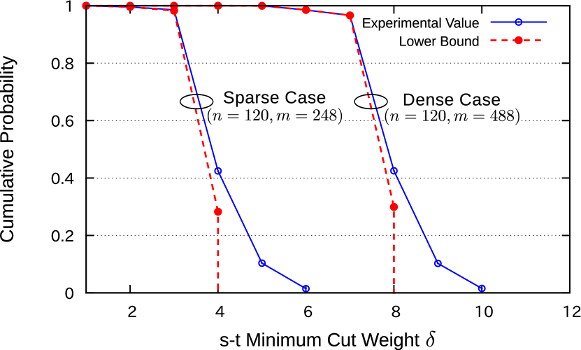
Figure 2: Accumulate distribution of the minimum $s{\mathchar 45\relax}t$ cut weight $\Pr(\lambda^{(s,t)}_{G}\geq\delta)$ (sparse case and dense case): experimental values and lower bounds.

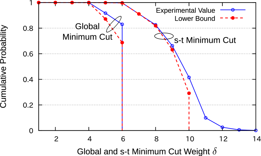
Figure 3: Accumulate distribution of the minimum $s{\mathchar 45\relax}t$ cut weight and the global minimum cut weight: experimental values and lower bounds.

VI Conclusion

In this paper, a lower bound on the accumulate distribution of the minimum $s{\mathchar 45\relax}t$ cut weight for a random graph ensemble is presented. From computer experiments, it is observed that the lower bound reflects actual statistical behavior of the minimum $s{\mathchar 45\relax}t$ cut weight. The proof technique used in this paper has close relationship to the analysis for average weight distribution of LDGM codes and it may be applicable to related problems on graphs such as the evaluation of the size of the minimum vertex cover over a random graph ensemble.

References

• [1] R.Β Ahlswede, S.-Y. Li, and R.Β Yeung, β€œNetwork information flow,” IEEE Transactions on Information Theory, vol.Β 46, no.Β 4, pp. 1204–1216, Jul. 2000.
• [2] A.Β Schrijver, Combinatorial Optimization: Polyhedra and Efficiency.Β Β Β Berlin: Springer-Verlag, 2003.
• [3] D.Β R. Karger, β€œRandom Sampling in Cut, Flow, and Network Design Problems,” Mathematics of Operations Research, vol.Β 24, no.Β 2, pp. 383–413, May 1999.
• [4] A.Β Ramamoorthy, J.Β Shi, and R.Β Wesel, β€œOn the Capacity of Network Coding for Random Networks,” IEEE Transactions on Information Theory, vol.Β 51, no.Β 8, pp. 2878–2885, Aug. 2005.
• [5] H.Β Wang, P.Β Fan, and K.Β Letaief, β€œMaximum flow and network capacity of network coding for ad-hoc networks,” IEEE Transactions on Wireless Communications, vol.Β 6, no.Β 12, pp. 4193–4198, Dec. 2007.
• [6] S.Β Hakimi and H.Β Frank, β€œCut-set matrices and linear codes,” IEEE Transactions on Information Theory, vol.Β 11, no.Β 3, pp. 457–458, Jul. 1965.
• [7] A.Β Yano and T.Β Wadayama, β€œProbabilistic analysis of the network reliability problem on a random graph ensemble,” in International Symposium on Information Theory and its Applications (ISITA), Oct. 2012, pp. 327 –331.
• [8] Y.Β Fujii and T.Β Wadayama, β€œA coding theoretic approach for evaluating accumulate distribution on minimum cut capacity of weighted random graphs,” in International Symposium on Information Theory and its Applications (ISITA), Oct. 2012, pp. 332 –336.
• [9] A.Β BarabΓ‘si and J.Β Frangos, Linked: The New Science Of Networks Science Of Networks.Β Β Β Perseus, 2002.
• [10] M.Β E.Β J. Newman, S.Β H. Strogatz, and D.Β J. Watts, β€œRandom graphs with arbitrary degree distributions and their applications,” Physical Review E, vol.Β 64, no.Β 2, pp. 026 118–, Jul. 2001.
• [11] C.-H. Hsu and A.Β Anastasopoulos, β€œAsymptotic Weight Distributions of Irregular Repeat-Accumulate Codes,” in Global Telecommunications Conference, 2005, pp. 1147–1151.