A Verified Approach for Checking Real-Time Specification Patterns

Abstract

We propose a verified approach to the formal verification of timed properties using model-checking techniques. We focus on properties expressed using real-time specification patterns, which can be viewed as a subset of timed temporal logics that includes properties commonly found during the analysis of reactive systems. Our model-checking approach is based on the use of observers in order to transform the verification of timed patterns into the verification of simpler LTL formulas. While the use of observers for model-checking is quite common, our contribution is original in several ways. First, we define a formal framework to verify that our observers are correct and non-intrusive. Second, we define different classes of observers for each pattern and use a pragmatic approach in order to select the most efficient candidate in practice. This approach is implemented in an integrated verification tool chain for the Fiacre language.

1 Introduction

distinctive feature of real-time systems is to be subject to severe time constraints that arise from critical interactions between the system and its environment. Since reasoning about real-time systems is difficult, it is important to be able to apply formal validation techniques early during the development process and to define formally the requirements that need to be checked.

In this work, we follow a classical approach to model checking: (1) we use a high-level language to describe a model of the system; (2) we use a logical-based formalism to express requirements on the system; and (3) the verification consists in compiling the system’s model and requirements into a low-level model for which we have the appropriate theory and the convenient tooling. We propose a new treatment for this traditional approach. In particular, for point (2), we focus on a dense real-time model and we use real-time patterns for the specification of the system instead of timed extensions of temporal logic. Our patterns can be interpreted as a real-time extension to the specification patterns of Dwyer et al. (1999). Time patterns can be used to express constraints on the timing as well as the order of events, such as the compliance to deadline or minimum time bounds on the delay between events. Concerning verification, point (3), we work with Time Transition Systems (see Sect. 2), an extension of Time Petri Nets with data variables and priorities.

Our first contribution is to propose a decidable verification method for checking real-time patterns on Time Transition Systems (TTS). The method is based on the use of observers and model-checking techniques in order to transform the verification of patterns into the verification of simpler LTL formula. Our observers are proved correct and non-intrusive, meaning that they compute the correct answer and have no impact on the system under observation. This is why we say our approach is verified. The formal framework we have defined is not only useful for proving the validity of formal results but also to check the soundness of optimisation in the implementation.

Our second contribution is to provide a reference implementation for these timed patterns. The complete framework defined in this paper has been integrated into a verification tool chain for Fiacre (Berthomieu et al., 2008), a high-level modelling language that can be compiled to TTS. Fiacre can be used as input language for two verification toolboxes: TINA, the TIme Petri Net Analyzer tool set (Berthomieu et al., 2004), and CADP (Garavel et al., 2011). In our tool chain (described in Fig. 1) a Fiacre specification is combined with patterns and compiled into a TTS model using the Frac compiler (the Fiacre language compiler). Then the model can be checked using the TINA toolbox. This is not a toy example. Indeed, Fiacre is the intermediate language used for model verification in Topcased (Farail et al., 2006), an Eclipse based toolkit for critical systems, where it is used as the target of model transformation engines from various languages, such as SDL, BPEL or AADL (Berthomieu et al., 2009). Therefore, through the connection with Fiacre, we can check timed patterns on many different modelling languages.

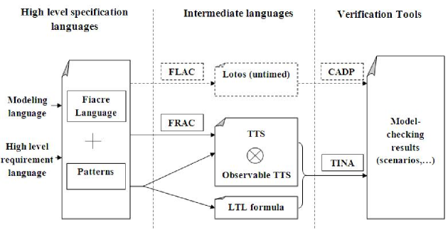
Figure 1: The global verification tool chain

Due to space limitations, we only give a partial descriptions of our timed patterns and give only part of our theoretical results. A complete catalogue of timed specification patterns is given in Abid et al. (2011a), while the complete formal framework is defined in a long version of this paper (Abid et al., 2011b).

For the purpose of this work, we focus on a simple deadline pattern, named $\mathop{\text{{{leadsto}\,}}}$, and define different classes of observers that can be used to check this pattern. We define observers for the $\mathop{\text{{{leadsto}\,}}}$ patterns that are based on the monitoring of places or transitions. In addition to these two traditional kind of observers, we propose a class of TTS observers that monitor data modifications. The goal is to choose the most efficient observer in practice. We give some experimental results on the impact of the choice of observer on the size of the state graphs that need to be generated—that is on the space complexity of our verification method—and on the verification time. The goal of this particular study is not to define a method for automatically generating an observer from a pattern. Instead, we define a set of possible observers that are compared in order to choose the best one in practice.

Outline

The paper is organised as follows. We start by introducing our formal framework in Sect. 2. This section is useful to define the notion of composition and non-interference for our observers. In Sect. 3 and 4, we describe a subset of our real-time specification patterns and the verification framework. We describe the implementation of our tool chain and give some experimental results on the use of the $\mathop{\text{{{leadsto}\,}}}$ pattern in Sect. 5. We conclude with a review of the related work, an outline of our contributions and some perspectives on future work.

2 Formal framework

We define some formal notations that are used in the remainder of this paper. In our approach, the observers and the systems are presented as Time Transition System (TTS), an extension of Time Petri Nets (TPN) see e.g. Merlin, 1974 with data variables and priorities. Our formal framework is based on the work of Peres et al. (2011), where the authors define formally the composition of two TPN. Their presentation has been extended to the full TTS model in Abid et al. (2011b).

The notion of composition is important in our work since we use TTS models for both the system and the observer and, for verification, we use TTS composition to graft the system with the observer.

This section is organised as follows: first, we introduce informally a TTS example. Then, we give a formal definition of TPN following the presentation of Peres et al. (2011), which is then extended to TTS. The semantics of TTS is defined using sets of timed traces. Finally, we define the composition of two TTS.

2.1 Informal Presentation of the TTS Model

We introduce next a graphical syntax of TTS using a simple example that models the behaviour of a mouse button with double-clicking, as pictured in Fig. 2. The behaviour, in this case, is to emit the event double if there are more than two click events in strictly less than one unit of time (u.t.).

Figure 2: The double-click example in TTS

Ignoring at first side conditions and side effects (the $\mathop{\text{{{pre}\,}}}$ and $\mathop{\text{{{act}\,}}}$ expressions inside dotted rectangles), the TTS in Fig. 2 can be viewed as a TPN with one token in place $s_{0}$ as its initial marking. From this “state”, a click transition may occur and move the token from $s_{0}$ to $s_{1}$. With this marking, the internal transition $\tau$ is enabled and will fire after exactly one unit of time, since the token in $s_{1}$ is not consumed by any other transition. Meanwhile, the transition labeled click may fire one or more times without removing the token from $s_{1}$, as indicated by the read arc (arcs ending with a black dot). After exactly one unit of time, because of the priority arc (a dashed arrow between transitions), the click transition is disabled until the token moves from $s_{1}$ to $s_{2}$.

Data is managed within the $\mathop{\text{{{act}\,}}}$ and $\mathop{\text{{{pre}\,}}}$ expressions that may be associated to each transition. These expressions may refer to a fixed set of variables that form the store of the TTS. Assume $t$ is a transition with guards $\mathop{\text{{{act}\,}}}$_t and $\mathop{\text{{{pre}\,}}}$_t. In comparison with a TPN, a transition $t$ in a TTS is enabled if there is both: (1) enough tokens in the places of its pre-condition; and (2) the predicate $\mathop{\text{{{pre}\,}}}$_t is true. With respect to the firing of $t$, the main difference is that we modify the store by executing the action guard $\mathop{\text{{{act}\,}}}$_t. For example, when the token reaches the place $s_{2}$ in the TTS of Fig. 2, we use the value of the variable dbl to test whether we should signal a double click or not.

2.2 Labeled Time Petri Nets and Time Transition Systems

Labeled Time Petri Nets (or TPN) extend Time Petri Nets (Merlin, 1974) with an action alphabet and a function labelling the transitions with those actions.

Notation : Let $I^{+}$ be the set of nonempty real intervals with non negative rational endpoints. For $i\in I^{+}$ , the symbol $\mathop{\downarrow}\kern-1.72218pti$ denotes the left end-point of the interval $i$ and $\mathop{\uparrow}\kern-1.72218pti$ its right end-point, if $i$ is bounded, or $\infty$ otherwise. We use ${\rm Nature}$ to denote the set of non negative integers.

Definition 1

A labeled Time Petri Net (or TPN) is a 8-tuple $(P,T,B,F,M_{0},I_{s},\sum,L)$ in which:

• $P$ is a finite set of places $p_{i}$;

• $T$ is a finite set of transitions $t_{i}$;

• $B$ is the backward incidence function
  $B:T\rightarrow P\rightarrow{\rm Nature};$

• $F$ is the forward incidence function
  $F:T\rightarrow P\rightarrow{\rm Nature};$

• $M_{0}$ is the initial marking function
  $M_{0}:P\rightarrow{\rm Nature};$

• $I_{s}$ is a function called the static interval function
  $I_{s}:T\rightarrow I^{+};$
  Function $I_{s}$ associates a temporal interval $I_{s}(t)\in I^{+}$ with every transition of the system. $\mathop{\downarrow}\kern-1.72218ptI_{s}(t)$ and $\mathop{\uparrow}\kern-1.72218ptI_{s}(t)$ are called the static earliest and latest firing times of $t$, respectively. Assuming that a transition t became enabled at time $\tau$, then $t$ cannot fire before $(\tau+\mathop{\downarrow}\kern-1.72218ptI_{s}(t))$ and no later than $(\tau+\mathop{\uparrow}\kern-1.72218ptI_{s}(t))$ unless disabled by firing some other transition.

• $\sum$ is a finite set of actions, or labels, not containing the silent action $\varepsilon$;

• $L:T\rightarrow\sum\cup\{\varepsilon\}$ is a transition labelling function.

A marking is a function $M:P\rightarrow{\rm Nature}$ that records the current (dynamic) value of the places in the net, as transitions are fired. The transition $t\in T$ is enabled by $M$ iff $(M\geqslant B(t))$. The dynamic interval function $I:T\rightarrow I^{+}$ is a mapping from transitions to time intervals. The dynamic interval function is used to record the current timing constraints associated to each transition, as time passes.

A transition $t$ can fire from $(M,I)$ if $t$ is enabled at $M$ and instantly fireable, that is $0\in I(t)$. In the target state, the transitions that remained enabled while $t$ is fired ($t$ excluded) keep their time interval, the intervals of the others (newly enabled) transitions are set to their respective static intervals. Together with those “discrete” transitions, a time Petri Net adds the ability to model the flowing of time. A transition of amount $d$ (i.e. taking $d$ time units) is possible iff $d$ is less than $\mathop{\uparrow}\kern-1.72218ptI(t)$ for all enabled transitions $t$.

The definition of TTS is a natural extension of TPN that takes variables and priorities into account. Details are presented in Abid et al. (2011b).

Definition 2 (Timed traces)

A timed trace $\sigma$ is a possibly infinite sequence of events $t\in T$ and duration $d$ with $d\in^{+}$. Formally, $\sigma$ is a partial mapping from ${\rm Nature}$ to $\dot{T}=T\cup\,{\{d\mid d\in^{+}\}}$ such that $\sigma(i)$ is defined whenever $\sigma(j)$ is defined and $i\leq j$.

The domain of $\sigma$ is written $\mathop{\mathsf{dom}}\sigma$. If $\mathop{\mathsf{dom}}\sigma$ is finite, the duration of $\sigma$, denoted $\Delta(\sigma)$, is the sum of the delays in $\sigma$, that is $\sum_{i\mid\sigma(i)\in^{+}}\sigma(i)$.

The semantics of a TPN (resp. TTS) is the set of its timed traces. (see details in Abid et al. (2011b)).

2.3 Composition of TTS and Timed Traces

We study the composition of two TTS and consider the relation between traces of the composed system and traces of both components. This operation is particularly significant in the context of this work, since both the system and the observer are TTS and we use composition to graft the latter to the former. In particular, we are interested in conditions ensuring that the behaviour of the observer does not interfere with the behaviour of the observed system.

The “parallel composition” of labeled Petri nets is a fundamental operation that is used to model large systems by incrementally combining smaller nets. Basically, the composition of two labeled TPN $N_{1}$ and $N_{2}$ is a labeled net $N\smash[t]{{\overset{\text{def}}{=}}}(N_{1}\parallel N_{2})$ such that: the places of $N$ is the cartesian product of the places of $N_{1}$ and $N_{2}$, and the transitions of $N$ is the fusion of the transitions in $N_{1}$ and $N_{2}$ that have the same label. A formal definition for the composition of two TPN is given in Peres et al. (2011). Composition of TTS is basically the same (Abid et al., 2011b), with the noticeable restriction that transitions which have priority over other transitions may not be synchronised across components. This is required to ensure the compositionality theorem, which we introduce below.

In the same way, we can define the composition of timed traces as an operation that builds a timed trace $\sigma_{1}\parallel\sigma_{2}$ from two traces $\sigma_{1}$ and $\sigma_{2}$. The trace $\sigma_{1}\parallel\sigma_{2}$ is obtained by merging the events with the same labels. This operation is well-defined for pairs of composable traces. Let $N_{1}$ (resp. $N_{2}$) be a TPN, and $\sigma_{1}$ (resp. $\sigma_{2}$) one of its traces. We say that $\sigma_{1}$ and $\sigma_{2}$ are composable iff $\mathop{\mathsf{dom}}{\sigma_{1}}=\mathop{\mathsf{dom}}{\sigma_{2}}$, and for all $i\in\mathop{\mathsf{dom}}{\sigma_{1}}$, (1) $\sigma_{1}(i)=d\wedge d\in^{+}\Rightarrow\sigma_{2}(i)=d$, and (2) $\sigma_{1}(i)=t\wedge t\in T\Rightarrow L(\sigma_{1}(i))=L(\sigma_{2}(i))$.

The compositionality theorem states that the behaviour of the composed system (expressed as a set of timed traces) is a subset of the behaviour of both components. In other terms, composing a system with an observer cannot generate new behaviour.

Theorem 1 (Compositionality)

Let $N_{1}$ and $N_{2}$ be two TTS and $N=N_{1}\parallel N_{2}$ be their composition. Then, for every timed trace $\sigma$ of $N$, there exist two timed traces, $\sigma_{1}$ and $\sigma_{2}$, such that: (1) $\sigma_{i}$ is a trace of $N_{i}$ for $i\in 1..2$ and (2) $\sigma=\sigma_{1}\parallel\sigma_{2}$.

In the compositionality theorem, the trace $\sigma_{1}$ (resp. $\sigma_{2}$) is obtained from $\sigma$ by “erasing” all transitions of $N_{2}$ (resp. $N_{1}$). Due to lack of space, we omit the proof here and invite the reader to consult Abid et al. (2011b).

3 Real-Time Specification Patterns

We have defined in Abid et al. (2011a) a set of specification patterns that can express constraints on the delays between the occurrences of two events or on the duration of a given condition. In our context, the event of a model can be: a transition that is fired; the system entering or leaving a state; a change in the value of variables; …The advantage of proposing predefined patterns is to provide a simple formalism to non-experts for expressing properties that can be directly checked with our verification tool chain. Our patterns can be viewed as a real-time extension of Dwyer’s (1999) specification patterns. In his seminal work, Dwyer shows through a study of 500 specification examples that 80% of the temporal requirements can be covered by a small number of “pattern formulas”. We follow a similar philosophy and define a list of patterns that takes into account timing constraints. At the syntactic level, this is mostly obtained by extending Dwyer’s patterns with two kind of timing modifiers: (1) $P$ $\mathop{\text{{{within}\,}}}$ $I$, which states that the delay between two events declared in the pattern $P$ must fit in the time interval $I$; and (2) $P$ $\mathop{\text{{{lasting}\,}}}$ $D$, which states that the condition defined by $P$ must hold for at least duration $D$. For example, we define a pattern $\mathop{\text{{{Present}\,}}}$ $A$ $\mathop{\text{{{after}\,}}}$ $B$ $\mathop{\text{{{within}\,}}}$ $]0,4]$ to express that the event $A$ must occur within 4 unit of time of the first occurrence of event $B$, if any, and not simultaneously with it. Although seemingly innocuous, the addition of these two modifiers has a great impact on the semantics of patterns and on the verification techniques that are involved.

We describe our patterns using a hierarchical classification borrowed from Dwyer et al. (1999), with patterns arranged in categories such as universality, absence, response, etc. In the following, we give some examples of absence and response patterns based on the TTS example of Fig. 2. Each of these patterns can be checked using our tool chain. A complete catalogue of patterns, with their formal definition, is given in Abid et al. (2011a). In this section, we focus on the “response pattern with delay”, to give an example of how patterns can be formally defined and to explain our different classes of observers.

3.1 Absence Pattern with Delay

This category of patterns is used to specify delays within which activities must not occur. A typical pattern in this category is:

$$\mathop{\text{{{absent}\,}}}E_{2}\mathop{\text{{{after}\,}}}E_{1}\mathop{\text{{{for interval}\,}}}[d_{1};d_{2}]\leavevmode\nobreak\ ,$$

which asserts that a transition (labeled with) $E_{2}$ cannot occur between $d_{1}$ and $d_{2}$ units of time after the first occurrence of a transition $E_{1}$. An example of use for this pattern would be the requirement that we cannot have two double clicks in less than $2$ units of time (u.t.), that is: $\mathop{\text{{{absent}\,}}}$ double $\mathop{\text{{{after}\,}}}$ double $\mathop{\text{{{for interval}\,}}}$ $[0;2]$. (This property is not true for our example in Fig. 2.) A more contrived example is to require that if there are no single clicks in the first $10$ u.t. of an execution then there should be no double clicks at all. This requirement can be expressed using the composition of two absence patterns using the implication operator and the reserved transition init (that identifies the start of the system):

$$\begin{array}[]{l}\big{(}\mathop{\text{{{absent}\,}}}{\textsf{{single}}}\mathop{\text{{{after}\,}}}{\textsf{{init}}}\mathop{\text{{{for interval}\,}}}[0;10]\big{)}\\ \quad\Rightarrow\big{(}\mathop{\text{{{absent}\,}}}{\textsf{{double}}}\mathop{\text{{{after}\,}}}{\textsf{{init}}}\mathop{\text{{{for interval}\,}}}[0;\infty[\big{)}\leavevmode\nobreak\ .\end{array}$$

3.2 Response Pattern with Delay

This category of patterns is used to express that some (triggering) event must always be followed by a given (response) event within a fixed delay of time. The typical example of response pattern states that every occurrence of a transition labeled with $E_{1}$ must be followed by an occurrence of a transition labeled with $E_{2}$ within a time interval $I$. (We consider the first occurrence of $E_{2}$ after $E_{1}$.)

$$E_{1}\mathop{\text{{{leadsto}\,}}}E_{2}\mathop{\text{{{within}\,}}}I\leavevmode\nobreak\ .$$

For example, using a disjunction between transition labels, we can bound the time between a click and a mouse event with the pattern: click $\mathop{\text{{{leadsto}\,}}}$ $({\textsf{{single}}}\vee{\textsf{{double}}})$ $\mathop{\text{{{within}\,}}}$ $[0,1]$.

3.3 Other Examples of Patterns

To give a feel of the expressiveness of our patterns, we briefly describe some other examples. For each pattern, we give just a textual definition. In each example, $E_{1}$, $E_{2}$ and $E_{3}$ refer to events in the system and $d_{1}$ (resp. $d_{2}$) stand for the left end-point (resp. right end-point) of the time interval $I$.

Predicate $E_{1}$ must hold between $d_{1}$ and $d_{2}$ u.t after the first occurrence of $E_{2}$. The pattern is also satisfied if $E_{2}$ never holds.

The first occurrence of $E_{1}$ should be between $d_{1}$ and $d_{2}$ u.t. before the first occurrence of $E_{2}$. The pattern also holds if $E_{2}$ never occurs.

Starting from the first occurrence when the predicate $E_{1}$ holds, it remains true for at least duration $D$. This pattern makes sense only if $E_{1}$ is a predicate on states (that is, on the marking or store); since transitions are instantaneous, they have no duration.

No $E_{1}$ can occur less than $D$ u.t. before the first occurrence of $E_{2}$. The pattern holds if there are no occurrence of $E_{2}$.

Before the first occurrence of $E_{3}$, each occurrence of $E_{1}$ is followed by an occurrence of $E_{2}$ which occurs both before $E_{3}$, and in the time interval $I$ after $E_{1}$. The pattern holds if $E_{3}$ never occurs.

Same than with the pattern “$E_{1}$ $\mathop{\text{{{leadsto first}\,}}}$ $E_{2}$ $\mathop{\text{{{within}\,}}}$ $I$” but only considering occurrences of $E_{1}$ after the first $E_{3}$.

3.4 Interpretation of Patterns

We can use different formalisms to define the semantics of patterns. In this work, we focus on a denotational interpretation, based on first-order formulas over timed traces (with equality and trace composition). We illustrate our approach using the pattern $E_{1}\mathop{\text{{{leadsto}\,}}}E_{2}\mathop{\text{{{within}\,}}}I$.

For the “denotational” definition, we say that the pattern $E_{1}\mathop{\text{{{leadsto}\,}}}E_{2}\mathop{\text{{{within}\,}}}I$ is true for a TTS $N$ if and only if, for every timed-trace $\sigma$ of $N$, we have:

$$\forall\sigma_{1},\sigma_{2}\ .\ (\sigma=\sigma_{1}E_{1}\sigma_{2})\Rightarrow\left(\begin{array}[c]{@{}l@{}}\exists\sigma_{3},\sigma_{4}\ .\ \sigma_{2}=\sigma_{3}E_{2}\sigma_{4}\\ \quad\wedge\Delta(\sigma_{3})\in I\wedge E_{2}\notin\sigma_{3}\end{array}\right)$$

where $\Delta(\sigma_{3})$ is the sum of all the duration in $\sigma_{3}$. The denotational approach is very convenient for a “tool developer” (for instance to prove the soundness of an observer implementing a pattern) since it is self-contained.

For another example, the denotational definition for the pattern $\mathop{\text{{{absent}\,}}}E_{2}\mathop{\text{{{after}\,}}}E_{1}\mathop{\text{{{for interval}\,}}}I$ is given by the following condition on the traces $\sigma$ of a system:

$$\begin{array}[c]{l@{}l}\forall\sigma_{1},\sigma_{2},\sigma_{3}\ .&(\sigma=\sigma_{1}E_{1}\sigma_{2}E_{2}\sigma_{3})\\ &\ \wedge(E_{1}\notin\sigma_{1})\Rightarrow(\Delta(\sigma_{2})\notin I)\end{array}$$

On our complete catalogue of patterns (Abid et al., 2011a), we provide an alternative (equivalent) semantics for patterns based on MTL, a timed extension of linear temporal logic see e.g. Maler et al., 2006 for a definition of the logic. For instance, for the leadsto pattern, the equivalent MTL formula is $\oblong\big{(}E_{1}\Rightarrow((\neg E_{2})\mathrel{\mathbf{{U}}}_{I}E_{2})\big{)}$, which reads like a LTL formula enriched by a time constraint on the until modality $\mathrel{\mathbf{{U}}}$.

4 Patterns Verification

We define different types of observers at the TTS level that can be used for the verification of patterns. It is important to note that we do not give an automatic method to generate observers. Rather, we define a set of observers for each patterns and, after selecting the “most efficient one”, we prove that it is correct (see the discussion in Sect. 5). We make use of the whole expressiveness of the TTS model to build observers: synchronous or asynchronous rendez-vous (through places and transitions); shared memory (through data variables); and priorities. We believe that an automatic method for generating the observer, while doable, will be detrimental for the performance of our approach. Moreover, when compared to a “temporal logic” approach, we are in a more favorable situation because we only have to deal with a finite number of patterns.

4.1 Observers for the Leadsto Pattern

We focus on the example of the leadsto pattern. We assume that some events of the system are labeled with $E_{1}$ and some others with $E_{2}$. We give three examples of observers for the pattern: $E_{1}$ leadsto $E_{2}$ within $[0,\mathit{max}[$. The first observer monitors transitions and uses a single place; the second observer monitors places; the third observer monitors shared, boolean variables injected into the system (by means of composition). We define our TTS observers using a classical graphical notation for Petri Nets, where arcs with a black circle denote read arcs, while arcs with a white circle are inhibitor arcs. (These extra categories of arcs can be defined in TTS and are supported in our tool chain.) The use of a data observer is quite new in the context of TTS systems. The results of our experiments seem to show that, in practice, this is the best choice to implement an observer.

4.1.1 Transition Observer

The observer $O_{t}$, see Fig. 3, uses a place, obs, to record the time since the last transition $E_{1}$ occurred. The place obs in $O_{t}$ is emptied if a transition labeled $E_{2}$ is fired, otherwise the transition error is fired after $\mathit{max}$ unit of time. The priority arc (dashed arrow) between error and $E_{2}$ is used to observe the transition error even in the case where a transition $E_{2}$ occurs exactly $\mathit{max}$ u.t. after the place obs was filled.

By definition of the TTS composition operator, the composition of the observer $O_{t}$ with the system $N$ duplicates each transitions in $N$ that is labeled $E_{1}$: one copy can fire if obs is empty—as a result of the inhibitor arc—while the other can fire only if the place is full. As a consequence, in the TTS $N\parallel O_{t}$, the transition error can fire if and only if the place obs stays full—there has been an instance of $E_{1}$ but not of $E_{2}$—for a duration of $\mathit{max}$. Then, to prove that $N$ satisfies the leadsto pattern, it is enough to check that the system $N\parallel O_{t}$ cannot fire the transition error. This can be done by checking the LTL formula $\oblong(\neg{\textsf{{error}}})$ on the system $N\parallel O_{t}$.

The observer $O_{t}$ given in Fig. 3 is deterministic and will “react” to the first occurrence of $E_{2}$ that miss a deadline. It is also possible to define a non-deterministic observer, such that some occurrences of $E_{1}$ or $E_{2}$ may be disregarded. This approach is safe since model-checking performs an exhaustive exploration of the states of the system; it considers all possible scenarios. This non-deterministic behaviour is quite close to the treatment obtained when compiling an (untimed) LTL formula “equivalent” to the leadsto pattern, namely $\oblong(E_{1}\Rightarrow\Diamond E_{2})$, into a Büchi automaton (Gastin et al., 2001). We have implemented the deterministic and non-deterministic observers and compared them taking in account their impact on the size of the state graphs that need to be generated and on the verification time. Experiments have shown that the deterministic observer is more efficient, which underlines the benefit of singling out the best possible observer and looking for specific optimisation.

Figure 3: Transition Observer: $O_{t}$

Figure 4: Data Observer: $O_{d}$

4.1.2 Data Observer

We define the data observer $O_{d}$ in Fig. 4. The data observer has a transition error conditioned by the value of a boolean variable, flag, that “takes the role” of the place obs in $O_{t}$ (every boolean variable is considered to be initially set to false). Indeed, flag is true between an occurrence of $E_{1}$ and the following transition $E_{2}$. Therefore, like in the previous case, to check if a system $N$ satisfies the pattern, it is enough to check the reachability of the event error. Notice that the whole state of the data observer is encoded in its store, since the underlying net has no place.

4.1.3 Place Observer

We define the place observer $O_{p}$ in Fig. 5. In this section, to simplify the presentation, we assume that the events $E_{1}$ and $E_{2}$ are associated to the system entering some given states $S_{1}$ and $S_{2}$. (But we can easily adapt this net to observe events associated to transitions in the system.) We also rely on a composition operator that composes TTS through their places instead of their transitions (Peres et al., 2011) and that is available in our tool chain. In $O_{p}$, we use a transition labeled $\tau_{1}$ whenever a token is placed in $S_{1}$ and a transition $\tau_{2}$ for observing that the system is in state $S_{2}$ (we assume that the labels $\tau_{1}$ and $\tau_{2}$ are fresh—private to the observer—and should not be composed with the observed systems). The remaining component of $O_{p}$ is just like the transition observer. We consider both a place and a transition observer since, depending on the kind of events that are monitored, one variant may be more efficient than the other.

Figure 5: Place Observer: $O_{p}$

4.2 Proving Innocuousness and Soundness of Observers

The goal of this section is to show how to prove that an observer for a pattern is correct. We demonstrate our approach on the particular examples of observers for the pattern $E_{1}\mathop{\text{{{leadsto}\,}}}E_{2}\mathop{\text{{{within}\,}}}[0,\mathrm{max}[$, given in the previous section.

We say that an observer $O$ for this pattern is sound if it can “detect” the traces of a system $N$ that do not hold for the pattern. More formally, if there is a trace $\sigma$ of $N$ such that: $\sigma=\sigma_{1}E_{1}\sigma_{2}E_{2}\sigma_{3}$ with $\Delta(\sigma_{2})\geq\mathrm{max}$ and $E_{2}\notin\sigma_{2}$, then there should be a trace $\sigma^{\prime}$ in $N\parallel O$ such that $\textsf{error}\in\sigma^{\prime}$. (The condition on the trace $\sigma$ directly follows from the denotational definition of the pattern, see Sect. 3.4) On the opposite, the observer is correct if it can detect that a system satisfies a pattern: if for all trace $\sigma^{\prime}$ of $N\parallel O$ we have $\textsf{error}\notin\sigma^{\prime}$ then for all trace $\sigma$ of $N$ the pattern holds.

From our compositionality theorem, see Sect. 2.3, we have that every trace $\sigma^{\prime}$ of $N\parallel O$ can be defined as the composition $\sigma\parallel\sigma_{o}$ of a trace $\sigma$ of the system $N$ with a trace $\sigma_{o}$ of the observer $O$. Therefore, to prove that an observer is correct, it is enough to prove that the pattern does not hold for a trace $\sigma_{o}$ in $O$ iff $\textsf{error}\in s_{o}$. Indeed, if there is a trace $\sigma$ in $N$ that does not hold for the pattern, then we obtain a trace $\sigma\parallel\sigma_{o}$ in $N\parallel O$ that does not hold either.

We can use our formal framework to prove the soundness of an observer (work is currently under way to mechanise these proofs using the Coq interactive theorem prover). Correctness proofs are more complicated, since they require to reason on the traces of a system composed with the observer to figure out the behaviour of the system alone. Therefore, instead of proving that an observer is correct, we prove a stronger assumption, that is that observers should be innocuous. A net is said to be innocuous if it cannot interfere with a system placed in parallel. More formally, the TTS $O$ is innocuous if for all TTS $N$ and for all trace $\sigma$ in $N$ there exists a trace $\sigma_{o}$ in $O$ such that $\sigma\parallel\sigma_{o}$ is a trace in $N\parallel O$. Innocuousness means that the observer cannot restrict the behaviour of another system. This is particularly useful in our case since, with innocuous observer, any trace $\sigma$ of the observed system $N$ is preserved in the composed system $N\parallel O$: the observer does not obstruct the behaviour of the system (see Lemma 1 below).

Instead of proving that observers are non-intrusive in a case by case basis, we can give a set of sufficient conditions for an observer $O$ to be innocuous. These conditions are met by the three observers given in Fig. 3–5.

Given a TTS $N$, we say that a transition $t$ of the observer is synchronised when there exists a labeled transition $t^{\prime}$ of $N$ such that $L(t)=L(t^{\prime})$ (and the label $L(t)$ is not $\epsilon$). We write $T_{sync}$ the set of synchronised transitions of the observer and $L_{sync}$ the labels of the synchronised transitions. The transitions in $T_{sync}$ are the transitions used by the observer to probe the system. In the examples defined in the previous section, the only synchronised transitions are the ones labeled $E_{1}$ and $E_{2}$ in the data ($O_{d}$) and transition ($O_{t}$) observers. We define $T_{imm}$ as the set of transitions of the observer whose static time interval is $[0,0]$. By construction, no transiton in $T_{sync}$ can also be part of $T_{imm}$.

Lemma 1

Assume $O$ satisfies the following three conditions:

• all synchronised transitions have a trivial static time interval and no priority (that is, for every $t$ in $T_{sync}$, $I_{s}^{t}=[0;+\infty[$ and $t$ has no priority over another transition in $O$);

• from any state of the observer, and for every label $l\in L_{sync}$, there is at least one transition $t$ in $O$ with label $l$ that can fire immediately;

• from any state of the observer, there is no infinite sequence of transitions in $T_{imm}$.

then, for all timed trace $\sigma$ in $N$ there exists a timed trace $\sigma\parallel\sigma_{o}$ in $N\parallel O$ such that $\sigma_{o}$ is a trace of $O$.

The proof of Lemma 1 can be found in Abid et al. (2011b). A few comments on these conditions. The first condition is necessary for defining the composition of two TTS (see Sect. 2.3). The second condition ensures that the observer cannot delay the firing of a synchronised transition “for a non-zero time”. Assume $s$ is a state of the observer $O$ and $\sigma$ a finite trace of $O$ starting from state $s$. We define $O(s,\sigma)$ to be the (necessarily unique) state reached by the observer after trace $\sigma$ has been executed. From the second condition, in every reachable state $s$ of $O$, and for every label $l$ in $L(T_{sync})$, there exists a (possibly empty) finite trace $\sigma$ not containing transitions in $T_{sync}$ such that the duration of $\sigma$ is 0 and there exists $t\in T_{sync}$ with $L(t)=l$, which is fireable in state $O(s,\sigma)$. Note also that the observer cannot involve other synchronised transitions while reaching a state where $l$ is firable, since this would abusively constrain the behaviour of the main system $N$, not to mention deadlock issues. This condition is true for the observer $O_{t}$ in Fig. 3 since, at any time, exactly one of the two transitions labeled $E_{1}$ (resp. $E_{2}$) can fire.

5 Experimental Results

Our verification framework has been integrated into a prototype extension of frac, the Fiacre compiler for the TINA toolbox. This extension supports the addition of real time patterns and automatically compose a system with the necessary observers. (Software and examples are available at http://homepages.laas.fr/~nabid.) In case the system does not meet its specification, we obtain a counter-example that can be converted into a timed sequence of events exhibiting a problematic scenario. This sequence can be played back using two programs provided in the TINA tool set, nd and play. The first program is a graphical animator for Time Petri Net, while the latter is an interactive (text-based) animator for the full TTS model.

We define the empirical complexity of an observer as its impact on the augmentation of the state space size of the observed system. For a system $S$, we define $\mathit{size}(S)$ as the size (in bytes) of the State Class Graph (SCG) (Berthomieu et al., 2004) of $S$ generated by our verification tools. In TINA, we use SCG as an abstraction of the state space of a TTS. State class graphs exhibit good properties: an SCG preserves the set of discrete traces—and therefore preserves the validation of LTL properties—and the SCG of $S$ is finite if the Petri Net associated with $S$ is bounded and if the set of values generated from $S$ is finite. We cannot use the “plain” labeled transition system associated to $S$ to define the size of $S$; indeed, this transition graph maybe infinite since we work with a dense time model and we have to take into account the passing of time.

The size of $S$ is a good indicator of the memory footprint and the computation time needed for model-checking the system $S$: the time and space complexity of the model-checking problem is proportional to $\mathit{size}(S)$. Building on this definition, we say that the complexity of an observer $O$ applied to the system $S$, denoted $C_{O}(S)$, is the quotient between the size of $(S\parallel O)$ and the size of $S$.

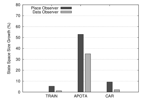
Figure 6: Compared complexity of the data and place observers (in percentage of system size growth)—average time for invalid properties (right) and valid properties (left).

We resort to an empirical measure for the complexity since we cannot give an analytical definition of $C_{O}$ outside of the simplest cases. However, we can give some simple bounds on the function $C_{O}$. First of all, since our observers should be non-intrusive, we can show that the SCG of $S$ is a sub graph of the SCG of $S\parallel O$, and therefore $C_{O}(S)\geq 1$. Also, in the case of the leadsto pattern, the transitions and places-based observers add exactly one place to the net associated to $S$. In this case, we can show that the complexity of these two observers is always less than $2$; we can at most double the size of the system. We can prove a similar upper bound for the leadsto observer based on data. While the three observers have the same (theoretical) worst-case complexity, our experiments have shown that one approach was superior to the others. We are not aware of previous work on using experimental criteria to select the best observer for a real-time property. In the context of “untimed properties”, this approach may be compared to the problem of optimising the generation of Büchi Automata from LTL formulas, see e.g. Gastin et al. (2001).

We have used our prototype compiler to experiment with different implementations for the observers. The goal is to find the most efficient observer “in practice”, that is the observer with the lowest complexity. To this end, we have compared the complexity of different implementations on a fixed set of representative examples and for a specific set of properties (we consider both valid and invalid properties). The results for the leadsto pattern are displayed in Fig. 6. For the experiments used in this paper, we use three examples of systems selected because they exhibit very different features (size of the state space, amount of concurrency and symmetry in the system, …):

• TRAIN is a model of a train gate controller. The example models a system responsible for controlling the barriers protecting a railroad crossing gate. When a train approaches, the barrier must be lowered and then raised after the train’s departure. The valid property, for the TRAIN example, states that the delay between raising and lowering a barrier does not exceed 100 unit of time. For the invalid property, we use the same requirement, but shortening the delay to 75.

• APOTA is an industrial use case that models the dynamic architecture for a network protocol in charge of data communications between an air plane and ground stations (Berthomieu et al., 2010). This example has been obtained using an translation from AADL to Fiacre. In this case, timing constraints arise from timeouts between requests and periods of the tasks involved in the protocol implementation. The property, in this case, is related to the worst-case execution time for the main application task.

• CAR is a system modelling an automated rail car system taken from Dong et al. (2008). The system is composed of four terminals connected by rail tracks in a cyclic network. Several rail cars, operated from a central control center, are available to transport passengers between terminals. When a car approaches its destination, it sends a request to the terminal to signal its arrival. Passengers in the terminal can then book a travel in the car. The valid property, for the CAR example, states that a passenger arriving in a terminal, must have a car ready to transport him within 15  unit of time. For the invalid property, we use the same requirement, but shortening the delay to 2 unit of time.

In Fig. 6, we compare the growth in the state space size—that is the value of $C_{o}(S)$—for the place and data observers defined in Sect. 4.1 and our three running examples. We do not consider the transition observer in these results since the events used in the requirements are all related to a system entering a state (and therefore our benchmark favor the place observer over the transition observer). We use one chart to display the result for patterns that are invalid and another for valid patterns.

In Fig. 7 (page 7), we give results on the total verification time for the APOTA example. The value displayed in the table refer to the time spent generating the complete state space of the system and verifying the property. The row SYSTEM gives the time needed for exploring the complete state space of the system (without adding any observer) while “VALID” and “INVALID” refer to the state space of the system synchronised with data observer and state observer in the case of valid and invalid property respectively.

In our experiments, we have consistently observed that the observer based on data is the best choice; it is the observer giving the minimal execution time in almost all the cases and that seldom gives the worst result. We can explain the efficiency of the data observer by the fact that it adds less transitions than the state observer; which means that it adds less intermediary states to the state space of $(N\parallel O)$.

Example	State observer	Data observer
SYSTEM	2.861	2.861
VALID	11.662	10.652
INVALID	11.611	10.179

Figure 7: Total verification time for APOTA (in seconds)

6 Related Work

Two broad approaches coexist for the definition and verification of real-time properties: (1) real-time extensions of temporal logic (Henzinger, 1998); and (2) observer-based approaches, such as the Context Description Languages (CDL) of Dhaussy et al. (Raji et al., 2010) or approaches based on timed automata (Maler et al., 2006; Aceto et al., 1998, 2003).

Obviously, the logic-based approach provides most of the theoretically well-founded body of works, such as complexity results for different fragments of real-time temporal logics (Henzinger, 1998): Temporal logic with clock constraints (TPTL); Metric Temporal Logic—with or without interval constrained operators—; Event Clock Logic; etc. The algebraic nature of logic-based approaches make them expressive and enable an accurate formal semantics. However, it may be impossible to express all the necessary requirements inside the same logic fragment if we ask for an efficient model-checking algorithm (with polynomial time complexity). For example, Uppaal (Behrmann et al., 2004) chose a restricted fragment of TCTL with clock variables, while Kronos provide a more expressive framework, but at the cost of a much higher complexity. As a consequence, selecting this approach requires to develop model-checkers for each interesting fragment of these logics—and a way to choose the right tool for every requirement—which may be impractical.

Pattern-based approaches propose a user-friendly syntax that facilitates their adoption by non-experts. However, in the real-time case, most of these approaches lack in theory or use inappropriate definitions. One of our goal is to reverse this situation. In the seminal work of Dwyer et al. (1999), patterns are defined by translation to formal frameworks, such as LTL and CTL. There is no need to provide a verification approach, in this case, since efficient model-checkers are available for these logics. This work on patterns has been extended to the real-time case. For example, Konrad et al. (2005) extends the patterns language with time constraints and give a mapping from timed pattern to TCTL and MTL, but they do not study the decidability of the verification method (the implementability of their approach). Another related work is (Gruhn et al., 2006), where the authors define observers based on Timed Automata for each pattern. However, they do not provide a formal framework for proving the correctness or the innocuousness of their observers and they have not integrated their approach inside a model-checking tool chain.

Concerning observer-based approaches, Aceto et al. (2003, 1998) use test automata to check properties of reactive systems. The goal is to identify properties on timed automata for which model checking can be reduced to reachability checking. In this framework, verification is limited to safety and bounded liveness properties. In the context of Time Petri Net, a similar approach has been experimented by Toussaint et al. (1997), but they propose a less general model for observers and consider only two verification techniques over four kinds of time constraints. Bayse et al. (2005) propose a method to verify the correctness of their approach formally. However, they do not prove formally all their invariants (patterns in our case).

7 Contributions and Perspectives

In contrast to these related works, we make the following contributions. We reduce the problem of checking real-time properties to the problem of checking LTL properties on the composition of the system with an observer. We define also a real-time patterns language based on the work of Dwyer et al. (1999) and inspired from real-case studies. To choose the best way to verify a pattern, we defined, for each pattern, a set of non-intrusive observers. We are based on a formal framework to verify the correctness of an observer, whether it can interfere with the behaviour of the system under observation.

Our approach has been integrated into a complete verification tool chain for the Fiacre modelling language and can therefore be used in conjunction with Topcased (Farail et al., 2006). We give several experimental results based on the use of this tool chain in Sect. 5. The fact that we implemented our approach has influenced our definition of the observers. Indeed, another contribution of our work is the use of a pragmatic approach for comparing the effectiveness of different observers for the same property. Our experimental results seem to show that data observers look promising.

We are following several directions for future work. A first goal is to define a new low-level language for observers—adapted from the TTS model—equipped with more powerful optimisation techniques and with easier soundness proofs. On the theoretical side, we are currently looking into the use of mechanised theorem proving techniques to support the validation of observers. On the experimental side, we need to define an improved method to select the best observer. For instance, we would like to provide a tool for the “syntax-directed selection” of observers that would choose (and even adapt) the right observers based on a structural analysis of the target system.

References

- Abid et al. (2011a) Abid, N. and Dal Zilio, S. and Le Botlan, D. (2011) A Real-Time Specification Patterns Language. LAAS Tech. Report 11364.
- Abid et al. (2011b) Abid, N. and Dal Zilio, S. and Le Botlan, D. (2011) Verification of Real-Time Specification Patterns on Time Transitions Systems. LAAS Tech. Report 11365.
- Aceto et al. (1998) Aceto, L. and Burgueño, A. and Larsen, K. (1998). Model Checking via Reachability Testing for Timed Automata. In proc. of TACAS’98–4th Int. Conf. on Tools and Alg. for Constr. and Analysis of Systems.
- Aceto et al. (2003) Aceto, L. and Bouyer, P. and Burgueño, A. and Larsen, K. (2003). The power of reachability testing for timed automata. Theor. Comput. Sci.
- Bayse et al. (2005) Bayse, E. and Cavalli, A. and Nunez, M. and Zaïdi, F. (2005). A passive testing approach based on invariants: application to the WAP. Int. Journal of Computer and Telecommunications Networking.
- Behrmann et al. (2004) Behrmann, G. and David, A. and Larsen, K. (2004). A Tutorial on Uppaal. Theor. Comput. Sci
- Berthomieu et al. (2004) Berthomieu, B. and Ribet, P.-O. and Vernadat, F. (2004) The tool TINA–Construction of Abstract State Spaces for Petri Nets and Time Petri Nets Int. Journal of Production Research.
- Berthomieu et al. (2008) Berthomieu, B. and Bodeveix, J.P. and Farail, P. and Filali, M. and Garavel, H. and Gaufillet, P. and Lang, F. and Vernadat, F. (2008) Fiacre: an Intermediate Language for Model Verification in the Topcased Environment ERTS 2008.
- Berthomieu et al. (2009) Berthomieu, B. and Bodeveix, J-P. and Chaudet, C. and Dal Zilio, S. and Filali, M. and Vernadat, F. (2009). Formal Verification of AADL Specifications in the Topcased Environment Int. Journal of Production Research.
- Berthomieu et al. (2010) Berthomieu, B. and Bodeveix, J-P. and Dal Zilio, S. and Dissaux, P. and Filali, M. and Heim, S. and Gaufillet, P. and Vernadat, F. (2010) Formal Verification of AADL models with Fiacre and Tina, 5th Int. Congress and Exhibition on Embedded Real-Time Software and Systems.
- Dong et al. (2008) Dong, J. S. and Hao, P. and Qin, S. C. and Sun, J. and Yi, W (2008) Timed automata patterns, IEEE Transactions on Software Engineering, 52(1), 2008.
- Dwyer et al. (1999) Dwyer, M-B. and Avrunin, G-S and Corbett, J.C (1999) Patterns in Property Specifications for Finite-State Verification ICSE, pp.411-420.
- Farail et al. (2006) Farail, P. and Gaufillet, P. and Canals, A.and Le Camus, C. and Sciamma, C. and Michel, P. and Crégut, X. and Pantel, M. (2006) The TOPCASED project: a Toolkit in OPen source for Critical Aeronautic SystEms Design, In Proc. of ERTS—Embedded Real Time Software.
- Garavel et al. (2011) Garavel, H. and Lang, F. and Mateescu, R. and Serwe, W. (2011) CADP 2010: A Toolbox for the Construction and Analysis of Distributed Processes, In Proc. of TACAS—17th Int. Conf. on Tools and Algorithms for the Construction and Analysis of Systems.
- Gastin et al. (2001) Gastin, P. and Oddoux, D. (2001) Fast LTL to Büchi Automata Translation, In Proc. of CAV—13th Int. Conf. on Computer Aided Verification.
- Gruhn et al. (2006) Gastin, P. and Oddoux, D. (2006) Patterns for Timed Property Specifications, Electr. Notes Theor. Comput. Sci., pp.117-133.
- Henzinger (1998) Henzinger, T-H. (1998) It’s About Time: Real-Time Logics Reviewed, 9th Int. Conf. on Concurrency Theory.
- Konrad et al. (2005) Konrad, S. and Cheng, B-H-C. (2005) Real-time specification patterns, 27th Int. Conf. on Software Engineering.
- Maler et al. (2006) Maler, O. and Nickovic, D. and Pnueli, A. (2005) From MITL to Timed Automata, 4th Int. Conf. on Formal Modeling and Analysis of Timed Systems.
- Merlin (1974) Merlin, P-M. (1974) A study of the recoverability of computing systems, PhD thesis, Dept. of Inf. and Comp. Sci., Univ. of California, Irvine, CA, 1974.
- Peres et al. (2011) Peres, F. and Berthomieu B. and Vernadat, F. (2011) On the composition of time Petri nets, journal Discrete Event Dynamic Systems.
- Raji et al. (2010) Raji, A. and Dhaussy, P. and Aizier, B. (2010) Automating Context Description for Software Formal Verification, Workshop MoDeVVa
- Toussaint et al. (1997) Toussaint, J. and Simonot-Lion, F. and Thomesse, J-P. (1997) Time Constraints Verification Methods Based on Time Petri Nets, 6th IEEE Workshop on Future Trends of Distributed Computer Systems.