Finite Length Analysis on Listing Failure Probability of Invertible Bloom Lookup Tables

Abstract

The Invertible Bloom Lookup Tables (IBLT) is a data structure which supports insertion, deletion, retrieval and listing operations of the key-value pair. The IBLT can be used to realize efficient set reconciliation for database synchronization. The most notable feature of the IBLT is the complete listing operation of the key-value pairs based on the algorithm similar to the peeling algorithm for low-density generator-matrix (LDGM) codes. In this paper, we will present a stopping set (SS) analysis for the IBLT which reveals finite length behaviors of the listing failure probability. The key of the analysis is enumeration of the number of stopping matrices of given size. We derived a novel recursive formula useful for computationally efficient enumeration. An upper bound on the listing failure probability based on the union bound accurately captures the error floor behaviors. It will be shown that, in the error floor region, the dominant SS have size 2. We propose a simple modification on hash functions, which are called SS avoiding hash functions, for preventing occurrences of the SS of size 2.

I Introduction

The Invertible Bloom Lookup Tables (IBLT) is a recently developed data structure which supports insertion, deletion, retrieval and listing operations of the key-value pairs [7]–[10]. The IBLT can be seen as a natural extension of the Bloom filter [1]–[6] which can handle set membership queries. The most notable feature of the IBLT is the complete listing operation of the key-value pairs based on the algorithm similar to the peeling algorithm [12] for low-density generator-matrix (LDGM) codes.

The listing operation enable us to use the IBLT for a basis of an efficient set reconciliation algorithm with small amount of communications. Set reconciliation is a process to synchronize contents of two sets at two distinct locations and it can be used for realizing database synchronization, memory synchronization, and an implementation of the Biff codes [10]. The implementation of the IBLT is fairly simple and it is naturally scalable to multiple servers, which is a desirable feature for data sets of extremely large size.

The paper by Goodrich and Mitzenmacher [7] provides the detailed analysis on the IBLT such as the optimization of the number of hash functions to minimize the retrieval failure probability. They also presented asymptotic thresholds for accurate recovery by using the known results on 2-cores of random hypergraphs. Furthermore, some fault tolerance features of the IBLT are extensively studied.

For designing practical applications, it is beneficial to know not only the asymptotic behavior of listing processes but also finite length performances. Especially, predicting the error floor of the listing failure probability is required to guarantee the accuracy of a listing process. It is known stopping sets [11] dominate the finite length performance of LDGM codes for erasure channels. In the case of the IBLT, the stopping sets have crucial importance as well as the case of LDGM codes. In this paper, we will present a stopping set analysis for the IBLT which unveils the finite length behaviors of the listing failure probability.

The outline of this manuscript is organized as follows. Section II introduces notation and definitions required for this paper. A brief review of the IBLT is also given. Section III provides an upper bound on the listing failure probability. An enumeration method for the number of stopping matrices based on a recursive formula is the heart of the efficient evaluation of the upper bound. Section IV presents some results of computer experiments. It will be shown that, in the error floor region, the stopping sets with size 2 become dominant. In Section V, a class of hash functions, SS avoiding hash functions, is proposed to resolve the stopping sets with size 2 for lowering the error floor.

II Preliminaries

II-A Bloom Filter

Before going into details of the IBLT, we here explain the structure of the original Bloom filter (BF) which is the basis of the IBLT. Assume that we have a binary array $T$ and $k$-hash functions $h_{1},\ldots,h_{k}$. The binary array $T$ is initially set to all zero. When an item $x$ comes to insert, we set $T[h_{i}(x)]=1$ for $i\in[1,k]$. The notation $[\alpha,\beta]$ means the set of consecutive integers from $\alpha$ to $\beta$. The process is called the Insert$(x)$ operation. The set membership query on $y$ is the query for checking whether $y$ is in the BF or not. The LookUp$(y)$ operation returns YES if $T[h_{i}(y)]=1$ for $i\in[1,k]$; otherwise it returns NO. The operations Insert$(x)$ and LookUp$(y)$ can be carried out in $O(k)$-time. Note that the LookUp$(y)$ operation may yield false positive; i.e., it returns YES when $y$ is not in the BF. The minimization of this false positive probability in terms of the number of hash functions is an important topic of studies of the BF [1][6]. An appropriately designed BF provides a highly space efficient set membership query system with reasonably small false positive probability.

II-B IBLT and its Operations

As in the case of the BF, $k$-hash functions $h_{1},\ldots,h_{k}$ are used in the IBLT. Instead of binary array, the IBLT utilizes an array of cells $T[1],\ldots,T[m]$. A cell $T[i]$ consists of three fields which are called Count, KeySum, and ValueSum, which are denoted by $T[i].Count,T[i].KeySum,T[i].ValueSum$. An input to the IBLT is a key-value pair $(Key,Value)$. The count field represents the number of inserted entries. The KeySum (resp. ValueSum) field stores exclusive OR of key (resp. value) of inserted entries. The contents of all the cells are initialized to zero at the beginning.

The IBLT allows 4-operations: Insert$(x,y)$, Delete$(x,y)$, Get$(x)$ and ListEntries$()$. The operation Insert$(x,y)$ stores a key-value pair $(x,y)$ into the IBLT. In an insertion process, the key $x$ (resp. value $y$) is added (over $\mathbb{F}_{2}$) to the KeySum (resp. ValueSum) filed of $T[h_{i}(x)]$ for $i\in[1,k]$; namely, $T[h_{i}(x)].KeySum=T[h_{i}(x)].KeySum\oplus x$ and $T[h_{i}(x)].ValueSum=T[h_{i}(x)].ValueSum\oplus y$. The count field of $T[h_{i}(x)]$ is also incremented as $T[h_{i}(x)].count=T[h_{i}(x)].count+1$ at the same time. The operation Delete$(x,y)$ removes the key-value pair $(x,y)$ from the IBLT. The process is the same as that of Insert$(x,y)$ except for decrementing the counter. The operation Get$(x)$ retrieves the value corresponding to the key $x$. This operation is realized as follows. If there exists $i\in[1,k]$ satisfying $T[h_{i}(x)].Count=1$, then Get$(x)$ returns $T[h_{i}(x)].ValueSum$. Otherwise, Get$(x)$ declares the failure of the operation.

The last operation ListEntries$()$ outputs all the key-value pairs in the IBLT by sequentially removing the entries with the counter value equal to one from the table. The details of the process is as follows. We first look for $i\in[1,m]$ satisfying $T[i].Count=1$. If there exists $i^{*}$ satisfying the condition $T[i^{*}].Count=1$, the key-value pair $(T[i^{*}].KeySum,T[i^{*}].ValueSum)$ is registered into the output list and then Delete$(T[i^{*}].KeySum,T[i^{*}].ValueSum)$ is executed. This process is iterated until no cell with the counter value equal to one can be found. It should be remarked that, in some cases, ListEntries$()$ fails to list all the entry in the IBLT. This is because a non-empty IBLT can have counter values larger than one for $i\in[1,m]$. This failure event is called a listing failure. It is desirable that an IBLT is designed to decrease the frequency of the listing failure events as small as possible.

II-C Probabilistic Model

It is clear that the probability of the listing failure event, which is called the listing failure probability, depends on the definition of the probabilistic model for keys and hash functions. In this paper (except for Section V), we assume the following model for keys and hash functions. The hash functions $h_{1},\ldots,h_{k}$ have domain $\{0,1\}^{b}$ and the key of the entries to be stored are independent random variables uniformly distributed over $\{0,1\}^{b}$. The number of entries are assumed to be $n$. The hash functions are assumed to be uniform such that $h_{i}(x)$ distributes uniformly in the range of $h_{i}$ when $x\in\{0,1\}^{b}$ obeys the uniform distribution. The $m$-cells are split into $k$-subtables each of size $m/k$ and each hash function uniformly selects a cell in a subtable. In other words, the range of $h_{i}$ is $[(i-1)*(m/k)+1,i*(m/k)]$.

III Upper Bound on Listing Failure Probability

In this section, we will derive an upper bound on the listing failure probability. The listing failure event occurs when a stopping set [11], which is a combinatorial substructure of a matrix, appears. In order to evaluate the listing failure probability, we need to enumerate the number of stopping matrices of given size. A stopping matrix is a matrix with no row of weight one corresponding to the case where no cells with counter value equal to one exists.

III-A Enumeration of Stopping Matrix

The state matrix $B$ of an IBLT can be represented by an $m\times n$ binary matrix where $m=\ell k$. A row of the matrix $B$ corresponds to a cell and a column corresponds to an entry. The matrix $B$ can be divided into disjoint $k$-blocks with size $\ell\times n$. If the $(s,t)$-element of the $u$-th block of $B$ is one, this means that the $t$-th entry is hashed to the $s$-th cell by using the $u$-th hash function. Suppose that a sub-matrix $M^{\prime}$ consisting of several columns of $M$ have no rows of weight one. In such a case, ListEntries$()$ fails to list all the entry in this table because $M^{\prime}$ cannot be resolved in the peeling process. If a binary matrix $M^{\prime}$ does not have a row with weight one, $M^{\prime}$ is said to be a stopping matrix. The existence of a stopping matrix in $B$ is the necessary and sufficient condition for the failure of a peeling process [11][12].

In our case, the state matrix $B$ is divided into $k$-subblocks corresponding to subtables. It might be reasonable to consider a stopping matrix in a subblock before discussing the probability of the event that $B$ includes a stopping matrix.

Let $S^{(\ell,n)}$ be the set of $\ell\times n$ binary matrices with column weight one; i.e.,

$$S^{(\ell,n)}\stackrel{{\scriptstyle\triangle}}{{=}}\{(m_{1},\ldots,m_{n})\in\{0,1\}^{\ell\times n}\mid wt(m_{i})=1,i\in[1,n]\},$$

where $wt(\cdot)$ represents the Hamming weight function. From this definition, it is evident that the cardinality of $S^{(\ell,n)}$ is $\ell^{n}$. The number of the stopping matrices in $S^{(\ell,n)}$ is denoted by $z(\ell,n)$, which can be written as

$$z(\ell,n)\stackrel{{\scriptstyle\triangle}}{{=}}\#\{M\in S^{(\ell,n)}\mid M\mbox{ is a stopping matrix}\}.$$ (1)

For convention, $z(0,0)$ is defined to be 1.

The next recursive formula plays a key role to enumerate $z(\ell,n)$ which is required for evaluating an upper bound for the listing failure probability.

Theorem 1 (Recursive formula on $z(\ell,n)$)

The following recursive relation

$$z(\ell,n)=\ell^{n}-\sum_{c=1}^{\min(\ell,n)}c!{\ell\choose c}{n\choose c}z(l-c,n-c)$$ (2)

holds for $\ell\geq 1$ and $n\geq 1$.

(Proof) Let $a(\ell,n)$ be the cardinality of non-stopping matrices $a(\ell,n)\stackrel{{\scriptstyle\triangle}}{{=}}\ell^{n}-z(\ell,n)$. In the following, we enumerate $a(\ell,n)$ by using a recursive relation. For given $M\in S^{(\ell,n)}$, a pair $(i,j)\in[1,\ell]\times[1,n]$ is said to be a pivot of $M$ if $M_{i,j}=1$ and the Hamming weight of the $i$-th row of $M$ is 1. The set of pivots of $M$ is denoted by

$$piv(M)\stackrel{{\scriptstyle\triangle}}{{=}}\{(i,j)\in[1,\ell]\times[1,n]\mid(i,j)\mbox{ is a pivot of }M\}.$$

Note that $M$ is a stopping matrix if and only if $piv(M)$ is empty. The cardinality of non-stopping matrices $a(\ell,n)$ can be represented by

$$a(\ell,n)=\sum_{i=1}^{\min(\ell,n)}\#T_{i}^{(\ell,n)}$$ (3)

where

$$T_{i}^{(\ell,n)}\stackrel{{\scriptstyle\triangle}}{{=}}\{M\in S^{(\ell,n)}\mid\#piv(M)=i\},\;i\in[0,\min(\ell,n)].$$ (4)

This is because the set of non-stopping matrices can be partitioned into disjoint sets $T_{i}^{(\ell,n)}$ for $i\in[1,\min(\ell,n)]$. In the following, we will try to prove the equality

$$\#T_{i}^{(\ell,n)}=c!{\ell\choose c}{n\choose c}z(l-c,n-c)$$ (5)

for $i\in[1,\min(\ell,n)]$. Assume that $M\in T_{c}^{(\ell,n)}$ is given ($c\in[1,\min(\ell,n)]$). By getting rid of all the column and rows corresponding to $piv(M)$ from $M$, we obtain an $(\ell-c)\times(n-c)$ matrix $M^{\prime}$. Namely we delete the $i$-th row and the $j$-th column from $M$ if $(i,j)\in piv(M)$. From the assumption $M\in T_{c}^{(\ell,n)}$, the resulting matrix $M^{\prime}$ must be a stopping matrix in $T_{0}^{(\ell-c,n-c)}$. Note that the size of $T_{0}^{(\ell-c,n-c)}$ is given by $z(\ell-c,n-c)$. Therefore, the size of $T_{i}^{(\ell,n)}$ is the product of the number of possible ways to choose $piv(M)$ and $z(\ell-c,n-c)$. Based on a simple combinatorial argument, we can see that the number of possible ways to choose $piv(M)$ can be enumerated as $c!{\ell\choose c}{n\choose c}$. As a result, we have the equality (5). Combining (3) and (5), the claim of the theorem is obtained. ∎

For some special combinations of $\ell$ and $n$, $z(\ell,n)$ has a simple expression as follows.

$$z(\ell,1) = 0,\quad\ell\geq 1$$ (6)

$$z(\ell,2) = \ell,\quad\ell\geq 1$$ (7)

$$z(\ell,3) = \ell,\quad\ell\geq 1$$ (8)

$$z(1,n) = 1,\quad n\geq 1.$$ (9)

These expressions can be easily proved based on the definition of the stopping matrix and of $S^{(\ell,n)}$. The recursive formula (2) enable us to evaluate the value of $z(\ell,n)$ efficiently. These simple expressions can be used as boundary conditions for a recursive evaluation process.

Table I presents the values of $z(\ell,n)$ for $(\ell,n)\in[1,10]^{2}$. These values are computed based on the recursive formula (2). Note that $S^{(\ell,n)}$ contains $10^{10}$-matrices when $\ell=n=10$. A naive enumeration scheme generating all the matrices in $S^{(\ell,n)}$ may have computational difficulty even for such small parameters.

TABLE I: Values of $z(\ell,n)$: Number of Stopping Matrices in $S^{(\ell,n)}$

$\ell\>\backslash\,n$	1	2	3	4	5	6	7	8	9	10
1	0	1	1	1	1	1	1	1	1	1
2	0	2	2	8	22	52	114	240	494	1004
3	0	3	3	21	63	243	969	3657	12987	43959
4	0	4	4	40	124	664	3196	15712	79228	396616
5	0	5	5	65	205	1405	7425	44385	271205	1666925
6	0	6	6	96	306	2556	14286	100176	691146	4916436
7	0	7	7	133	427	4207	24409	196105	1471519	11773699
8	0	8	8	176	568	6448	38424	347712	2775032	24547664
9	0	9	9	225	729	9369	56961	573057	4794633	46341081
10	0	10	10	280	910	13060	80650	892720	7753510	81163900

III-B Listing Failure Probability and its Bound

The set of all the state matrix is defined as

$$B^{(\ell,n,k)}\stackrel{{\scriptstyle\triangle}}{{=}}\{(M_{1},\ldots,M_{k})^{T}\mid M_{i}\in S^{(\ell,n)},i\in[1,k]\}.$$ (10)

The cardinality of $B^{(\ell,n,k)}$ is $\ell^{nk}$. According to the scenario we have discussed in the previous section, we here define a probability space by assigning the equal probability $1/\ell^{nk}$ to each element in $B^{(\ell,n,k)}$.

Suppose that $P_{f}(\ell,n,k)$ represents the listing failure probability, which is the probability that ListEntries$()$ operation fails to list all the entries in the IBLT. The next theorem provides an upper bound on $P_{f}(\ell,n,k)$.

Theorem 2 (Upper bound on listing failure probability)

For given $\ell\geq 1,n\geq 1,k\geq 1$, the listing failure probability $P_{f}(\ell,n,k)$ can be upper bounded by

$$P_{f}(\ell,n,k)\leq\sum_{i=2}^{n}{n\choose i}\left(\frac{z(\ell,i)}{\ell^{i}}\right)^{k}.$$ (11)

(Proof) The peeling process of the ListEntries$()$ fails to recover all the entries in the IBLT if and only if $B\in B^{(\ell,n,k)}$ contains a stopping matrix as its sub-matrix. Thus, $P_{f}(\ell,n,k)$ can be characterized as

$$P_{f}(\ell,n,k)=Pr[B\mbox{ includes a stopping matrix}].$$ (12)

For an index set ${\cal I}\in 2^{[1,n]}$, let $B_{\cal I}$ be the sub-matrix of $B$ consisting of columns of $B$ with indices in ${\cal I}$. If $B_{\cal I}\mbox{ is a stopping matrix}$, then the index set ${\cal I}$ is said to be a stopping set. The probability $P_{f}(\ell,n,k)$ can be upper bounded as follows:

$$P_{f}(\ell,n,k) = Pr[B\mbox{ includes a stopping matrix}]$$ (13)

$$= Pr\left[\bigcup_{{\cal I}\in 2^{[1,n]}\backslash\emptyset}B_{\cal I}\mbox{ is a stopping matrix}\right]$$

$$\leq \sum_{{\cal I}\in 2^{[1,n]}\backslash\emptyset}Pr\left[{\cal I}\mbox{ is a stopping set}\right].$$

The last inequality is due to the union bound. From the definition of the probability space defined on $B^{(\ell,n,k)}$, the probability that ${\cal I}$ is a stopping set is given by

$$Pr\left[{\cal I}\mbox{ is a stopping set}\right]=\left(\frac{z(\ell,\#{\cal I})}{\ell^{\#{\cal I}}}\right)^{k}.$$ (14)

By using this equality, we have the following upper bound:

$$P_{f}(\ell,n,k) \leq \sum_{{\cal I}\in 2^{[1,n]}\backslash\emptyset}Pr\left[{\cal I}\mbox{ is a stopping set}\right]$$ (15)

$$= \sum_{i=1}^{n}\sum_{{\cal I}\in 2^{[1,n]}\backslash\emptyset}Pr\left[{\cal I}\mbox{ is a stopping set}\mid\#{\cal I}=i\right]$$

$$= \sum_{i=2}^{n}{n\choose i}\left(\frac{z(\ell,i)}{\ell^{i}}\right)^{k}.$$

In the last equality, we used the fact $z(\ell,1)=0$. ∎

IV Computer Experiments

In this section, we will present several results on computer experiments and on numerical evaluation of the upper bound presented in the previous section.

In order to examine the tightness of the bound, Figure 1 presents curves of the listing failure probability obtained by computer experiments (dashed line) and of the upper bound (solid line). These curves are plotted as functions of the number of cells $m$. The number of entries is $n=210$ and the symbol size of the key is $b=32$. In computer experiments, the number of trials is $10^{6}$. As a hash function, SHA-1[13] was used. The number of the hash functions assumed to be $k=3$. We used pseudorandom $32$-bit numbers for pseudorandom key-value pairs. It can be observed that the upper bound gives fairly tight estimation, as the number of cells $m$ increases. As in the case of LDPC codes, the error curve in Figure 1 exhibit both water fall and error floor phenomenon. This result indicates that the upper bound precisely captures the error floor behavior of the listing failure probability.

From the upper bound, it is possible to see a tradeoff between the water fall and error floor. Figure 2 presents the upper bounds for $k\in[3,6]$. The number of entries is $n=100$. A curve of the upper bound is plotted as a function of the number of cells $m$. We can observe that the listing failure probabilities in the error floor region can be decreased as the number of hash functions $k$ increases. On the other hand, increments of $k$ pushes the water falls to the right.

From the upper bound and some experimental results, we see that stopping sets of size 2 dominates the error floor behavior. Figure 3 presents the upper bound, the asymptote $P_{2}(\ell,n,k)$ defined by

$$P_{2}(\ell,n,k)\stackrel{{\scriptstyle\triangle}}{{=}}{n\choose 2}\left(\frac{z(\ell,2)}{\ell^{2}}\right)^{k}={n\choose 2}\frac{1}{\ell^{k}}$$ (16)

and the experimental value of the list error probability. The result suggest that the probability of occurrence of stopping set of size 2 determines the depth of an error floor.

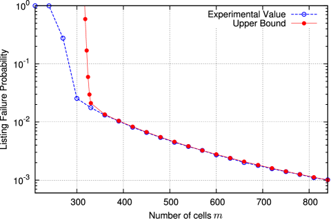
Figure 1: Comparison of the listing failure probability: experimental values and upper bound ($n=210,\;k=3,\;b=32$).

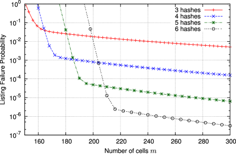
Figure 2: Comparison of the upper bound on listing failure probability: 3 hashes, 4 hashes, 5 hashes and 6 hashes ($n=100$).

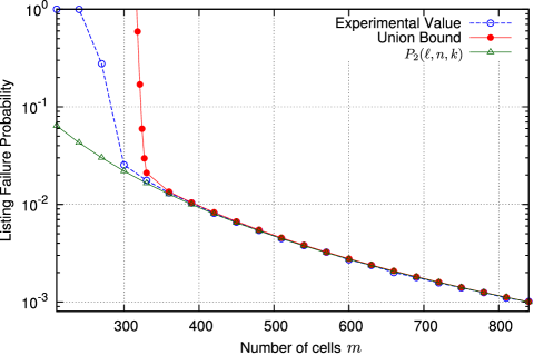
Figure 3: Comparison of the listing failure probability: experimental values, upper bound and asymptote $P_{2}(\ell,n,k)$ ($n=210,\;k=3,\;b=32$).

V SS Avoiding Hash Function

We have seen that stopping sets of size 2 dominate the behavior of the list failure probability in the error floor region. The stopping sets of size 2 occur when $k$-hash values for 2-distinct keys collide; i.e.,

$$(h_{1}(a),h_{2}(a),\ldots,h_{k}(a))=(h_{1}(b),h_{2}(b),\ldots,h_{k}(b))$$ (17)

for $a\neq b$. If this type of collision can be prevented, it is expected that the error floor performance can be improved.

The SS avoiding hash function defined here are designed so that the collisions (17) are avoided. In the following discussion, we will further assume the uniqueness of keys registered in the IBLT. Namely, an insertion of district entries with the same keys and a multiple insertion of the same key-value pairs are not allowed. This assumption may be natural for most of applications such as set reconciliation.

Let a hash function $h$ be an bijective map from $\{0,1\}^{b}$ to $\{0,1\}^{sk}$ where $b=sk$. The SS avoiding hash functions $(h_{1},\ldots,h_{k})$ are simply defined by partitioning the output $sk$-tuple from $h$ into $k$ binary $s$-tuples; i.e., $h_{i}(x)$ is given by

$$h_{i}(x)=q_{i}+(i-1)2^{s}+1,\quad i\in[1,k],$$ (18)

where $(q_{1},\ldots,q_{k})=h(x)(q_{i}\in\{0,1\}^{s})$. Note that $m/k=2^{s}$ holds; i.e., each subtable contains $2^{s}$-cells. Due to the assumption on the uniqueness of the keys in the IBLT, it is evident that a collision (17) does not occur. This means that occurrences of the stopping sets of size 2 can be completely prevented. Note that the use of the SS avoiding hash function introduces a restriction on several system parameters; i.e., $b=sk$. This inflexibility can be considered as a price to be paid for lowering the error floor.

It should be remarked that the probabilistic model assumed in Section II cannot be directly applied to the system presented in this section This is because the assumption on the uniqueness of the keys introduces weak correlations between the stored entries. Although we have to take care of these distinctions, the analysis presented in the previous sections may be still useful for predicting the performance of ListEntries$()$ with the SS avoiding hash functions if $b$ is large enough.

Figure 4 presents the results of a computer experiment on the SS avoiding hash functions. As an bijective map, the identity map was exploited. The two curves of listing failure probabilities are plotted; the first one corresponds to the case of a conventional hash function and the second one corresponds to the case of the SS avoiding hash function where the symbol size of the key is $b=3s$. In both cases, the number of entries is $n=210$ and the number of hash functions is assumed to be $k=3$. We can observe that the SS avoiding hash function reduces the listing failure probabilities in the error floor region. Furthermore, the upper bound almost captures the error floor behavior of the listing failure probability in this settings.

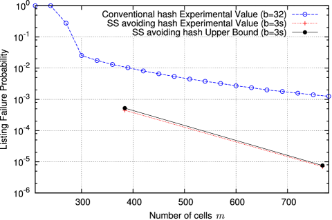
Figure 4: Comparison of the listing failure probability: conventional hash function and SS avoiding hash function ($n=210,\;k=3$).

VI Conclusion

In this paper, we presented a finite length performance analysis on the listing failure probability which may be useful for designing a system or an algorithm including the IBLT as a building component. The recursive formula presented in Section III will become an useful tool for finite length analysis. In Section IV, we have seen that the error floor performance can be improved by increasing the number of the hash functions but it degrades the waterfall performance. From the results shown in Section V, we can expect that appropriately designed SS avoiding hash functions can improve the error floor performance without sacrificing the waterfall performance.

References

- [1] B. Bloom, “Space/time trade-offs in hash coding with allowable errors,” Communications of the ACM, vol. 13, no. 7, pp. 422-426, 1970.
- [2] F. Bonomi, M. Mitzenmacher, R. Panigrahy, S. Singh, and G. Varghese, “Beyond Bloom filters: From approximate membership checks to approximate state machines,” ACM SIGCOMM Computer Communication Review, vol. 36, no. 4, pp. 326, 2006
- [3] F. Bonomi, M. Mitzenmacher, R. Panigrahy, S. Singh, and G. Varghese, “An improved construction for counting Bloom filters,” In Proceedings of the European Symposium on Algorithms (ESA), vol. 4168 of LNCS, pp. 684-695, 2006.
- [4] A. Broder and M. Mitzenmacher, “Network applications of Bloom filters: A survey,” Internet Mathematics, vol. 1, no. 4, pp. 485-509, 2004.
- [5] B. Chazelle, J. Kilian, R. Rubinfeld, and A. Tal, “The Bloomier filter: an efficient data structure for static support lookup tables,” In Proceedings of the Fifteenth Annual ACM-SIAM Symposium on Discrete Algorithms, pp. 30-39, 2004.
- [6] M. Mitzenmacher, “Compressed Bloom filters,” IEEE/ACM Transactions on Networking, vol. 10, no. 5, pp. 613-620, 2002.
- [7] M. Goodrich and M. Mitzenmacher, “Invertible bloom lookup tables,” In Proceedings of the 49th Allerton Conference, pp. 792-799, 2011.
- [8] F. Putze, P. Sanders, and J. Singler, “Cache-, hash-, and space-efficient Bloom filters,” ACM Journal of Experimental Algorithms, vol. 14, pp. 4.4-4.18, 2009.
- [9] D. Eppstein and M. T. Goodrich, “ Straggler identification in round-trip data streams via Newton’s identities and invertible Bloom filters,” IEEE Transactions on Knowledge and Data Engineering, vol. 23, no. 2, pp. 297-306, 2011.
- [10] M. Mitzenmacher, G. Varghese, “Biff (Bloom filter) codes: fast error correction for large data sets,” Information Theory Proceedings (ISIT), IEEE International Symposium on, pp. 483-487, 2012.
- [11] C. Di , D. Proietti , I.E.Teletar, T. Richardson and R. Urbanke, “Finite-length analysis of low-density parity-check codes on the binary erasure channel,” IEEE Transactions on Information Theory, vol. 48, no. 6, pp. 1570-1579, 2002.
- [12] T. Richardson and R. Urbanke, Modern Coding Theory, Cambridge University Press, 2008.
- [13] National Institute of Standards and Technologies, Secure Hash Standard, Federal Information Processing Standards Publication, FIPS-180, 1993.