Learning and inference in a nonequilibrium Ising model with hidden nodes

Abstract

We study inference and reconstruction of couplings in a partially observed kinetic Ising model. With hidden spins, calculating the likelihood of a sequence of observed spin configurations requires performing a trace over the configurations of the hidden ones. This, as we show, can be represented as a path integral. Using this representation, we demonstrate that systematic approximate inference and learning rules can be derived using dynamical mean-field theory. Although naive mean-field theory leads to an unstable learning rule, taking into account Gaussian corrections allows learning the couplings involving hidden nodes. It also improves learning of the couplings between the observed nodes compared to when hidden nodes are ignored.

I Introduction

Within the statistical mechanics community, a significant body of recent work deals with parameter learning in statistical models. This work typically focuses on the canonical setting of the inverse Ising problem: given a set of configurations from an equilibrium Kappen and Rodriguez (1998); *Tanaka98; *Roudi09-3; *Cocco2011adaptive; *Ricci2012; *Nguyen2012; *Nguyen2012PRL, or nonequilibrium Roudi and Hertz (2011a); *Mezard11; *Zeng11; *zhang2012inference Ising model, how can we find the interactions between the spins? These inverse problems can be difficult to solve using brute force approaches Ackley et al. (1985) and thus for practical purposes, the results of such theoretical works offering approximate learning and inference methods are of great importance. The recent interest in using statistical models to study high-throughput data from neural Schneidman et al. (2006); Shlens et al. (2006); Cocco et al. (2009), genetic Lezon et al. (2006) and financial Bury (2012) networks further emphasizes the necessity of developing efficient approximate inference methods.

Despite its practical relevance, however, little has been done on learning and inference in models with hidden spins using statistical physics. Learning the parameters of a statistical model in the presence of hidden nodes and inferring the state of hidden variables lie at the heart of difficult problems in statistics and machine learning. It is well known that for statistical modeling of data, hidden variables most often improve model quality Bishop (1999); Pearl (2000). Furthermore, when used for network reconstruction and graph identification, ignoring hidden nodes may cause the model to incorrectly identify/remove couplings between observed nodes when such couplings do not exist/actually exist. For these reasons, it is quite important to study models with hidden nodes, both from a theoretical perspective and for applications to real data where usually only a fraction of the system is observeable Schneidman et al. (2006); Shlens et al. (2006); Lezon et al. (2006).

In this paper, we study the reconstruction of the couplings in a nonequilibrium Ising model with hidden spins and the inference of the state of these spins. Theoretically, the couplings can be reconstructed by calculating and maximizing the likelihood of the data which involves performing a trace over the configurations of the hidden spins at all times: an impossible task even for moderately sized data sets and networks. This is, in fact, a general problem, not only for a nonequilibrium Ising model, but for any kinetic model with hidden variables. It is, however, natural to use a path integral approach for doing this trace, and this is what we do here. We show that efficient approximate learning and inference can be developed by evaluating the log-likelihood in this way and employing mean-field type approximations.

In what follows, after formulating the problem, we first evaluate the likelihood of the data using the saddle point approximation to the path integral. We find that the result allows inference of the state of hidden variables if the couplings are known but cannot be used for learning the couplings. We then perform a Gaussian correction to this saddle point approximation to derive Thouless-Anderson-Palmer (TAP) like equations Thouless et al. (1977) for our problem. Our numerical results show that successul learning of the couplings, even those that involve hidden nodes, can be achieved using the corrected learning rules. We find that with enough data and using these equations even hidden-to-hidden connections can be reconstructed.

Although in this paper our focus is on the paradigmatic case of the Ising model, the approach taken here is quite general and can be adapted to many other popular statistical models.

II Formulation of the problem

Consider a network of binary spin variables subject to synchronous update dynamics. Suppose some of these nodes are observed for $T$ time steps, while the other nodes are hidden. We denote the state of the observed spins at time $t$ by $\mbox{\boldmath$s$}(t)=\{s_{i}(t)\}$ and the hidden ones by $\mbox{\boldmath$\sigma$}=\{\sigma_{a}(t)\}$. For clarity, we always use the subscripts $i,j,\dots$ for the observed and $a,b,\dots$ for the hidden ones. We consider the following transition probability

$$p[\{\mbox{\boldmath$s$},\mbox{\boldmath$\sigma$}\}(t+1)|\{\mbox{\boldmath$s$},\mbox{\boldmath$\sigma$}\}(t)]=$$ (1a)

$$\hskip 30.0pt\exp[\sum\nolimits_{i}s_{i}(t+1)g_{i}(t)+\sum\nolimits_{a}\sigma_{a}(t+1)g_{a}(t)]Z(t)^{-1}$$

$$Z(t)=\prod_{i,a}2\cosh[g_{i}(t)]\ 2\cosh[g_{a}(t)]$$ (1b)

where $g_{i}(t)$ and $g_{a}(t)$ are the fields acting on observed spin $i$ and hidden spin $a$ at time $t$, respectively

$$g_{i}(t)=\sum\nolimits_{j}J_{ij}s_{j}(t)+\sum\nolimits_{b}J_{ib}\sigma_{b}(t)$$ (2a)

$$g_{a}(t)=\sum\nolimits_{j}J_{aj}s_{j}(t)+\sum\nolimits_{b}J_{ab}\sigma_{b}(t),$$ (2b)

$J_{ij},J_{ai},J_{ia}$ and $J_{ab}$ are the observed-to-observed, observed-to-hidden, hidden-to-observed and hidden-to-hidden connections. These couplings need not be symmetric and, thus, the network may never reach equilibrium. Although, here we consider the case of zero external field, our derivations follow also for nonzero fields.

Given this model, we would like to answer the following questions: What can we say about the state of hidden spins from the observations? How can we learn the various couplings in the network?

Answering these questions requires finding the likelihood of the data. Optimizing the likelihood with respect to $J$s yields the maximum likelihood value of the couplings. The posterior over the state of hidden nodes given the observed nodes is

$$p[\{\mbox{\boldmath$\sigma$}(t)\}^{T}_{t=1}|\{\mbox{\boldmath$s$}(t)\}^{T}_{t=1}]=\frac{p[\{\mbox{\boldmath$\sigma$}(t)\}^{T}_{t=1}\ ,\{\mbox{\boldmath$s$}(t)\}^{T}_{t=1}]}{p[\{\mbox{\boldmath$s$}(t)\}^{T}_{t=1}]}$$

which also requires calculating the likelihood.

The likelihood of the observed spin configurations under the model Eq. 1 is

$$p[\{\mbox{\boldmath$s$}(t)\}^{T}_{t=1}]={\rm Tr}_{\sigma}\prod_{t}p[\{\mbox{\boldmath$s$},\mbox{\boldmath$\sigma$}\}(t+1)|\{\mbox{\boldmath$s$},\mbox{\boldmath$\sigma$}\}(t)]$$ (3)

and involves a trace over $\{\mbox{\boldmath$\sigma$}(1),\dots,\mbox{\boldmath$\sigma$}(T)\}$ which is difficult to do.

To perform this trace analytically, we consider the following functional

$${\cal L}[\psi]\equiv\log{\rm Tr}_{\sigma}\prod_{t}e^{\sum_{a}\psi_{a}(t)\sigma_{a}(t)}p[\{\mbox{\boldmath$s$},\mbox{\boldmath$\sigma$}\}(t+1)|\{\mbox{\boldmath$s$},\mbox{\boldmath$\sigma$}\}(t)].$$ (4)

which, using the definition of the transition probability from Eq. 1, can be written as

$${\cal L}[\psi]=\log{\rm Tr}_{\sigma}\exp\left[Q[\mbox{\boldmath$s$},\mbox{\boldmath$\sigma$}]+\sum_{a,t}\psi_{a}(t)\sigma_{a}(t)\right]$$ (5)

$$Q=\sum_{i,t}s_{i}(t+1)g_{i}(t)+\sum_{a,t}\sigma_{a}(t+1)g_{a}(t)$$

$$\hskip 28.45274pt-\sum_{i,t}\log 2\cosh[g_{i}(t)]-\sum_{a,t}\log 2\cosh[g_{a}(t)].$$

The log-likelihood of the data is recovered at $\psi\to 0$. Furthermore, ${\cal L}[\psi]$ acts as the generating functional for the posterior over the hidden spins: $m_{a}(t)$, the mean magnetization of the hidden spin $a$ at time $t$ given the data, can be found using

$$m_{a}(t)=\lim_{\psi\to 0}\mu_{a}(\psi,t),\ \ \ \ \mu_{a}(\psi,t)=\frac{\partial{\cal L}[\psi]}{\partial\psi_{a}(t)}.$$ (6)

Higher-order derivatives of ${\cal L}$ with respect to $\psi$ yield higher-order correlation functions of the hidden spins.

To develop mean-field approximations, we first perform the trace in Eq. 5 using the standard approach for dealing with a nonlinear action in the local fields Coolen (2001); Opper and Winther (2001): we write the term inside the log in Eq. 5 as a path integral over $g_{i}(t)$ and $g_{a}(t)$ enforcing their definitions in Eq. 2 by inserting $\delta[g_{i}(t)-\sum_{j}J_{ij}s_{j}(t)-\sum_{b}J_{ib}\sigma_{b}(t)]$ and $\delta[g_{a}(t)-\sum_{j}J_{aj}s_{j}(t)-\sum_{b}J_{ab}\sigma_{b}(t)]$ in the integral. Using the integral representation of the delta functions, ${\cal L}$ can be written as

$${\cal L}[\psi]=\log\int D{\cal G}\exp[\Phi]$$ (7a)

$$\Phi=\log{\rm Tr}_{\mbox{\boldmath$\sigma$}}\exp[Q+\Delta+\sum_{a,t}\psi_{a}(t)\sigma_{a}(t)]$$ (7b)

where ${\cal G}=\{g_{i},\hat{g}_{i},g_{a},\hat{g}_{a}\}$. $\Delta$, as well as $\hat{g}_{i}$ and $\hat{g}_{a}$, come from the integral representation of the $\delta(\cdot)$ functions used to enforce the definitions in Eq. 2

$$\Delta=\sum_{i,t}i\hat{g}_{i}(t)[g_{i}(t)-\sum_{j}J_{ij}s_{j}(t)-\sum_{b}J_{ib}\sigma_{b}(t)]$$ (8)

$$\ \ \ \ \ +\sum_{a,t}i\hat{g}_{a}(t)[g_{a}(t)-\sum_{j}J_{aj}s_{j}(t)-\sum_{b}J_{ab}\sigma_{b}(t)]$$

The crucial thing about this rewriting of ${\cal L}$ is that the resulting action $\Phi$ is now linear in $\sigma$ and we can thus easily perform the trace over $\sigma$. The ability to perform the trace here comes at the cost of the high-dimensional integral over ${\cal G}$ in Eq. 7a. The integral, however, can be approximated using the saddle point approximation and the corrections to the saddle point.

III Saddle-point approximation

The saddle point values of $g_{a},g_{i},\hat{g}_{a}$ and $\hat{g}_{i}$ can be derived by putting the derivatives of $\Phi$ with respect to these variables to zero. For $\psi=0$, the saddle point equations read

$$i\hat{g}_{i}(t)=\tanh[g_{i}(t)]-s_{i}(t+1)$$ (9a)

$$i\hat{g}_{a}(t)=\tanh[g_{a}(t)]-m_{a}(t+1)$$ (9b)

$$g_{i}(t)=\sum\nolimits_{j}J_{ij}s_{j}(t)+\sum\nolimits_{b}J_{ib}m_{b}(t)$$ (9c)

$$g_{a}(t)=\sum\nolimits_{j}J_{aj}s_{j}(t)+\sum\nolimits_{b}J_{ab}m_{b}(t)$$ (9d)

in which $m_{a}(t)$ satisfy the self-consistent equations

$$m_{a}(t)=$$ (10)

$$\tanh\big{[}g_{a}(t-1)-i\sum\nolimits_{j}\hat{g}_{j}(t)J_{ja}-i\sum\nolimits_{b}\hat{g}_{b}(t)J_{ba}\big{]}$$

Let us take a moment to describe the physical meaning of these equations. The saddle point equations for $g_{i}$ and $g_{a}$, Eq. 9c and 9d, are just the mean values of the local fields at the mean magnetizations $m_{a}(t)$ of the hidden variables (see Eq. 2). Examining Eq. 9a and 9b, one can identify $-i\hat{g}_{i}(t)$ and $-i\hat{g}_{a}(t)$ as errors back propagated in time. The self-consistent equations for $m_{a}$, Eq. 10, take the form of the usual naive mean-field equations except that back propagated errors are taken into account.

Given a sequence of configurations from the observed spins, solving Eq. 10 yields the mean magnetization of the hidden ones given this data. The derivatives of $\Phi$ with respect to the $J$s, evaluated at the saddle point solutions, give the maximum likelihood learning rules for the couplings within this saddle point approximation.

IV Gaussian corrections

The saddle-point equations and learning rules can be improved by Gaussian corrections, that is by evaluating the contributions to the path integral from the Gaussian fluctuations around the saddle Negele and Orland (1998); Kholodenko (1990). This will lead to what can be called as TAP equations for our problem. In what follows, by doing this on the Legendre transform of ${\cal L}$,

$$\Gamma[\mu]={\cal L}-\sum_{a,t}\psi_{a}(t)\mu_{a}(t)$$ (11)

and using the equation of state,

$$-\psi_{a}(t)=\frac{\partial\Gamma[\mu]}{\partial\mu_{a}(t)}$$ (12)

we correct the naive mean-field equations for our problem with the hidden spins.

Denoting the saddle point value of ${\cal L}$ by ${\cal L}_{0}$, and performing a Legendre transform we have (see Appendix A)

$$\Gamma_{0}[\mu]=\sum_{i,t}[s_{i}(t+1)g_{i}(t)-\log 2\cosh(g_{i}(t))]$$ (13)

$$\ \ \ \ +\sum_{a,t}[\mu_{a}(t+1)g_{a}(t)-\log 2\cosh(g_{a}(t))]+\sum_{a,t}S[\mu_{a}(t)]$$

where $S[\mu_{a}(t)]$ is the entropy of a free spin with magnetization $\mu_{a}(t)$, and $g_{i}$ and $g_{a}$ are as in Eq. 2 with $\sigma_{b}(t)$ replaced by $\mu_{b}(t)$. Using Eq. 12 and putting $\psi=0$, we recover Eq. 10, as we should.

The Gaussian corrections can be performed as follows; for details see Appendix B. We first perform the Gaussian integral around the saddle point of ${\cal L}$. This modifies ${\cal L}_{0}$ to

$${\cal L}_{1}={\cal L}_{0}-\frac{1}{2}\log\det[\partial^{2}{\cal L}]$$ (14)

where $\partial^{2}{\cal L}$ is the Hessian, containing the second derivatives of ${\cal L}$ with respect to $g$ and $\hat{g}$, calculated at their saddle point values. Keeping terms quadratic in $J$ we then derive the modified equations for $m_{a}(t)$ by first calculating $\partial{\cal L}_{1}/\partial\psi_{a}(t)$. Expressing ${\cal L}_{1}$ in terms of the new $m_{a}(t)$, again keeping terms quadratic in $J$, and finally performing the Legendre transform, we get

$$\Gamma_{1}[m]=\Gamma_{0}[m]-\frac{1}{2}\sum_{i,a,t}[1-\tanh^{2}g_{i}(t)]J^{2}_{ib}[1-m^{2}_{b}(t)]$$

$$\hskip 11.38092pt-\frac{1}{2}\sum_{a,b,t}[m^{2}_{a}(t+1)-\tanh^{2}g_{a}(t)]J^{2}_{ab}[1-m^{2}_{b}(t)].$$ (15)

where now, $g_{i}$ and $g_{a}$ are as in Eq. 2 but with $m_{a}$ instead of $\sigma_{a}$. Eq. 15 together with the equation of state at $\psi\to 0$,

$$\frac{\partial\Gamma_{1}[m]}{\partial m_{a}(t)}=0,$$ (16)

yields the new self-consistent equation for $m_{a}(t)$. The couplings can then be found by optimizing $\Gamma_{1}$ with respect to the couplings.

In sum, the corrected TAP-learning will be the following EM like iterative algorithm: at each step, solve the equations for $m_{a}$ derived from Eq. 16 given the current value of the couplings, and then adjust the couplings proportional to $\partial\Gamma_{1}/\partial J$.

V Numerical results

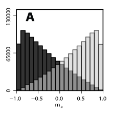
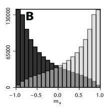
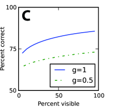
We evaluated the saddle point and TAP equations on data generated from a network of $N=100$ spins with the dynamics in Eq. 1 and with the couplings drawn independently from a Gaussian distribution with variance $J_{1}^{2}/N$. We first studied how much the saddle point Eq. 10 and TAP equations Eq. 16 tell us about the state of hidden spins if we know all the couplings. Fig. 1 A and B show the distributions of $m_{a}(t)$ when $20\%$ of the network is hidden. The solutions to the TAP equations are more pushed towards $+1$ and $-1$ compared to the saddle point. Using a simple estimator $\hat{\sigma}_{a}(t)=\mathop{\mathrm{sgn}}(m_{a}(t))$ to infer the state of hidden spin $a$ and time $t$, Fig. 1C shows that the two approximations perform equally well in inferring the state of hidden spins.

Figure 1: (Color online) Solutions for $m_{a}$. (A) and (B) show histograms of $m_{a}(t)$ found from solving saddle point and TAP equations, Eqs. 10, 16, given the correct couplings. Here we had $J_{1}=0.7$, $20\%$ hidden spins and a data length of $T=10^{5}$. The dark gray bars show the histogram of the values for which $\sigma_{a}(t)$ was actually $+1$ while the transparent ones show when it was actually $-1$. (C) shows the percent correct if we use $\hat{\sigma}_{a}(t)=\mathop{\mathrm{sgn}}(m_{a}(t))$ to infer the state of $\sigma_{a}(t)$ vs. the percentage of the visible part. TAP and saddle point results were virtually indistinguishable.

Figure 2: (Color online) Reconstructing the full network. Scatter plots showing the inferred couplings (blue dots) versus the correct ones in a network of $N=100$ total spins, with $10$ hidden, $J_{1}=1$ and data length of $T=10^{6}$. Red crosses show the initial values of the couplings used for learning. A, B, C, and D show observed-to-observed, observed-to-hidden, hidden-to-observed and hidden-to-hidden couplings, respectively.

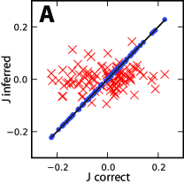
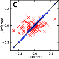
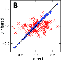
The effect of TAP corrections becomes very important in reconstructing the couplings. We found that the saddle point learning was always unstable leading to divergent couplings. However, including the TAP corrections dramatically changed this. Fig. 2 shows an example of this when $10\%$ of the spins were hidden. In this case, good reconstruction of all couplings could be achieved.

Figure 3: (Color online) Root mean squared error of the couplings. (A)-(C) show the rms error for the observed-to-observed, hidden-to-observed and observed-to-hidden couplings using TAP learning when the original model did not have hidden-to-hidden connections; the other couplings were drawn independently from a Gaussian. (D)-(F) show the same but when the hidden-to-hidden connections were present in the original network but were ignored (i.e. put to zero) when learning the other couplings. In (A) and (D) the green dots show the inferred couplings by maximizing the likelihood with hidden nodes completely ignored. Here we used $J_{1}=1,N=100,T=10^{6}$, and five different random realizations of the connectivity.

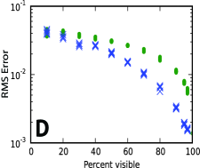
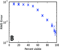
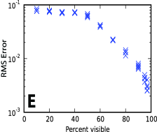
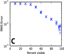
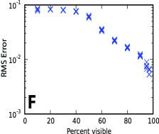
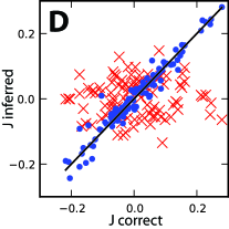
Although for a proportionally small number of hidden nodes we observed good reconstruction, when the hidden part was large, for a constant data length, we found that the algorithm starts to become unstable: the root mean squared error for the inferred hidden-to-hidden connections increases after a few iterations and the others follow. This instability, however, seems to arise from our attempt to learn the hidden-to-hidden connections. For an architecture where there is no hidden-to-hidden couplings, that is a dynamical semi-restricted Boltzmann machine Osindero and Hinton (2008); *taylor2009factored, or when hidden-to-hidden couplings exist in the original network but are ignored during learning (i.e. put to zero), the algorithm allows recovering the other connections even for very large hidden sizes. This is shown in Fig. 3.

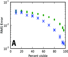
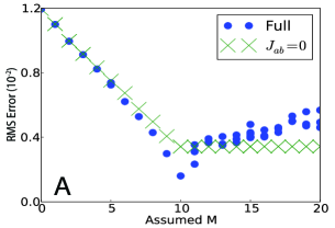
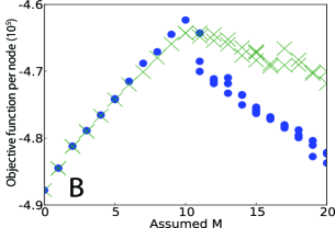
In the examples above, we have used the right number of hidden nodes when learning the couplings. In practice, however, the number of hidden nodes may be unknown. We thus wondered if the number of hidden nodes can be estimated from the data. In Fig. 4, we plot the objective function $\Gamma_{1}/N$ for the data used in Fig. 2, where $N$ is the total number of visible nodes, that is, the sum of the observed nodes, and an unknown number $M$ of hidden nodes. As can be seen in Fig. 4, varying $M$, at the correct number of hidden units a peak in $\Gamma_{1}/N$ is seen and also the reconstruction error of the visible-to-visible connectivity reaches a minimum. This was the case, even when we constrained the hidden-to-hidden connections to zero during learning. However, the peak in the normalized cost function was sharper, and the minmum achieved for the reconstruction lower, when hidden-to-hidden connections were also learned.

Figure 4: (Color online) Estimation of the number of hidden nodes. (A) the RMS error of the observed-to-observed couplings inferred using TAP learning for different values of assumed hidden units, $M$. The couplings are inferred either assuming no hidden-to-hidden connectivity (green x) or by trying to learn all couplings (blue circles). (B) the value of the objective function per inferred node for different numbers of assumed hidden units. The data used here is the same as that of Fig. 2, that is in reality there were $10$ hidden nodes which is where the normalized objective function shows maximum and the RMS error shows a minimum.

VI Discussions

In this paper we described an approach for learning and inference in a nonequilibrium Ising model when it is partially observed, that is, when the history of spin configurations are known only for some spins and not for the others. Treating the log-likelihood of the data as a path integral over the fields acting on hidden and observed spins in a non-equilibrium Ising model, we approximated it first using saddle point approximations, and then by considering TAP corrections to it.

In usual statistical mechanics settings, TAP equations can be derived in several ways: using Plefka expansion Plefka (1981); *Biroli99; *Roudi11-2, information-geometric arguments Kappen and Spanjers (2000) or by calculating the Gaussian fluctuations around the saddle point Kholodenko (1990); Negele and Orland (1998). Here we took an approach similar to the latter case except that we did not use the Hubbard-Stratonovich transformation. It would be quite interesting to see what the other approaches yield as TAP corrections. Tyrcha and Hertz Tyrcha and Hertz (2013) have also studied the problem of hidden spins, using a different approach. Their equations agree with ours at the saddle point level but differ at the TAP level.

In terms of performance, saddle point equations gave results that were similar to TAP for inferring the state of hidden spins, but were very unstable for learning the couplings. Using TAP equations, learning all the couplings, even the hidden-to-hidden ones, was possible when the hidden part was proportionally small. By ignoring hidden-to-hidden couplings, even when they were present in the network, we could achieve good performance in recovering all the other couplings, even with half the network hidden. This also improved recovering the observed-to-observed couplings compared to when hidden spins were ignored all together. Our numerical results also indicate that even the number of hidden units can be estimated by optimization of the objective function. This is of particular practical revelance as often the true size of the network is unknown. In Fig. 4, both the objective function and the reconstruction quality increase as we add hidden nodes suggesting that even a wrong number of hidden nodes can improve the reconstruction of observed-to-observed couplings. This can be explained by the fact that the added hidden variables, even if wrong in number, to some degree can explain the correlations induced by the hidden spins in the real network.

An important future direction, in our view, is to study how averaging the likelihood over some couplings, in particular the hard to infer hidden-to-hidden ones, given a prior over them, will influence the reconstruction of the other couplings. There is a large body of work where the path integral approach is used to study the disorder-averaged behavior of disordered systems De Dominicis (1978); *Sompolinsky81; Coolen (2001). The approach that we developed here can be easily combined with this work to average out some of the couplings.

VII Acknowledgement

We are most grateful to Joanna Tyrcha and John Hertz for constructive comments and for discussing their work with us, and Claudia Battistin for comments on the paper. Benjamin Dunn acknowledges the hospitality of NORDITA. We also acknowledge the computing resources provided by the University of Oslo and the Norwegian metacenter for High Performance Computing (NOTUR), Abel cluster.

Appendix A Legendre transform

Here we derive Eq. 13 in the main text. Starting from Eq. 7, we have

$${\cal L}[\psi]=\log\int D{\cal G}\exp[\Phi],$$ (I-1a)

$$\Phi=\sum_{i,t}s_{i}(t+1)g_{i}(t)+i\sum_{i,t}\hat{g}_{i}(t)\Big{[}g_{i}(t)-\sum_{j}J_{ij}s_{j}(t)\Big{]}+i\sum_{a,t}\hat{g}_{a}(t)\Big{[}g_{a}(t)-\sum_{i}J_{ai}s_{i}(t)\Big{]}-\sum_{i,t}\log 2\cosh[g_{i}(t)]$$

$$\hskip 56.9055pt-\sum_{a,t}\log 2\cosh[g_{a}(t)]+\sum_{a,t}\log 2\cosh\Big{[}g_{a}(t-1)-i\sum_{b}J_{ba}\hat{g}_{b}(t)-i\sum_{i}J_{ia}\hat{g}_{i}(t)+\psi_{a}(t)\Big{]}$$ (I-1b)

$$\mu_{a}(t)=\frac{\partial\Phi}{\partial\psi_{a}(t)}=\tanh\big{[}g_{a}(t-1)-i\sum_{j}\hat{g}_{j}(t)J_{ja}-i\sum_{b}\hat{g}_{b}(t)J_{ba}+\psi_{a}(t)\big{]},$$ (I-1c)

with the saddle point being at Eq. 9, with $\mu_{a}$ instead of $m_{a}$. Applying the following identity to the last sum in Eq. I-1b

$$\log 2\cosh[x]=S[\tanh[x]]+x\tanh[x]$$ (I-2)

$$S[x]\equiv-\frac{1+x}{2}\log\left[\frac{1+x}{2}\right]-\frac{1-x}{2}\log\left[\frac{1-x}{2}\right]$$ (I-3)

and using Eq. I-1c and the saddle point values for $g_{i}$ and $g_{a}$, we obtain

$$\Phi_{0}=\sum_{i,t}[s_{i}(t+1)g_{i}(t)-\log 2\cosh[g_{i}(t)]]$$

$$\hskip 28.45274pt+\sum_{a,t}[\mu_{a}(t+1)g_{a}(t)-\log 2\cosh[g_{a}(t)]]$$

$$\hskip 28.45274pt+\sum_{a,t}\mu_{a}(t)\psi_{a}(t)+\sum_{a,t}S[\mu_{a}(t)]$$ (I-4)

At the saddle point we have ${\cal L}_{0}=\Phi_{0}$ and using $\Gamma_{0}={\cal L}_{0}-\sum_{a,t}\psi_{a}(t)\mu_{a}(t)$ we arrive at Eq. 13.

Appendix B Corrections to the saddle-point likelihood

To include the Gaussian corrections in Eq. 15 we first calculate the Gaussian fluctuations around the saddle point value of ${\cal L}_{0}.$ Given Eq. I-1b, we have

$$A_{ij}^{tt^{\prime}}\equiv\frac{\partial^{2}\Phi}{\partial g_{i}(t)\partial g_{j}(t^{\prime})}=-\delta_{ij}\delta_{tt^{\prime}}[1-\tanh^{2}[g_{i}(t)]]$$

$$B_{ij}^{tt^{\prime}}\equiv\frac{\partial^{2}\Phi}{\partial\hat{g}_{i}(t)\partial\hat{g}_{j}(t^{\prime})}=-\sum\nolimits_{a}J_{ia}J_{ja}[1-\mu^{2}_{a}(t)]\delta_{tt^{\prime}}$$

$$C_{ab}^{tt^{\prime}}\equiv\frac{\partial^{2}\Phi}{\partial g_{a}(t)\partial g_{b}(t^{\prime})}$$

$$\hskip 56.9055pt=-\delta_{ab}\delta_{tt^{\prime}}\Big{[}\mu^{2}_{a}(t+1)-\tanh^{2}[g_{a}(t)]]\Big{]}$$

$$D_{ab}^{tt^{\prime}}\equiv\frac{\partial^{2}\Phi}{\partial\hat{g}_{a}(t)\partial\hat{g}_{b}(t^{\prime})}=-\sum\nolimits_{c}J_{ac}J_{bc}[1-\mu^{2}_{c}(t)]\delta_{tt^{\prime}}$$

$$E_{ib}^{tt^{\prime}}\equiv\frac{\partial^{2}\Phi}{\partial\hat{g}_{i}(t)\partial\hat{g}_{b}(t^{\prime})}=-\sum\nolimits_{a}J_{ia}J_{ba}[1-\mu^{2}_{a}(t)]\delta_{t,t^{\prime}}$$

$$F_{ib}^{tt^{\prime}}=\frac{\partial^{2}\Phi}{\partial\hat{g}_{i}(t)\partial g_{b}(t^{\prime})}=-iJ_{ib}[1-\mu^{2}_{b}(t)]\delta_{t-1,t^{\prime}}$$

$$\frac{\partial^{2}\Phi}{\partial g_{a}(t)\partial\hat{g}_{b}(t^{\prime})}=i\delta_{ab}\delta_{tt^{\prime}}\underbrace{-iJ_{ba}[1-\mu^{2}_{a}(t+1)]\delta_{t^{\prime},t+1}}_{G_{ab}}$$

and $\partial^{2}\Phi/\partial g_{i}(t)\partial\hat{g}_{j}(t^{\prime})=i\delta_{ij}\delta_{tt^{\prime}}$leading to

$$\left[\BMAT{cc.cc|cc.cc}{cc.cc|cc.cc}A^{tt}&i\mathbb{1}000000\\ i\mathbb{1}B^{tt}0E^{tt}0000\\ 00C^{tt}i\mathbb{1}0[F^{t^{\prime}t}]^{T}0G^{tt^{\prime}}\\ 0[E^{tt}]^{T}i\mathbb{1}D^{tt}0000\\ 0000A^{t^{\prime}t^{\prime}}i\mathbb{1}00\\ 00F^{t^{\prime}t}0i\mathbb{1}B^{t^{\prime}t^{\prime}}0E^{t^{\prime}t^{\prime}}\\ 000000C^{t^{\prime}t^{\prime}}i\mathbb{1}\\ 00[G^{tt^{\prime}}]^{T}00[E^{t^{\prime}t^{\prime}}]^{T}i\mathbb{1}D^{t^{\prime}t^{\prime}}\\ \right]$$ (II-2)

as part of the Hessian for $t$ and $t^{\prime}=t+1$, and the same structure gets repeated for other times. The first to the fourth rows/columns correspond to derivatives with respect to $g_{i},\hat{g}_{i},g_{a},\hat{g}_{a}$ all at $t$ and the fourth to eighth rows/columns at $t^{\prime}=t+1$.

Denoting the matrix of the blocks on the diagonal part of the Hessian as $\alpha$ and the rest as $\beta$, we write

$$\log\det(\alpha+\beta)=\log\det(\alpha)+\log\det[I+\alpha^{-1}\beta]$$

$$=\log\det(\alpha)+{\rm Tr}\log[I+\alpha^{-1}\beta]$$ (II-3)

$$\approx\log\det(\alpha)+{\rm Tr}[\alpha^{-1}\beta]+\frac{1}{2}{\rm Tr}\{[\alpha^{-1}\beta]^{2}\}\}+\cdots$$

Assuming that the couplings are random and independent with mean of order $1/N$ and a standard deviation of $J_{1}/\sqrt{N}$ as typically assumed in mean-field models of spin glasses Fischer and Hertz (1991), $\log\det(\alpha)$ will be of quadratic order in $J_{1}$. Since $\alpha$ is block diagonal, so will be $\alpha^{-1}$ and therefore ${\rm Tr}[\alpha^{-1}\beta]=0$. Ignoring the second trace as contributing higher order terms, we thus approximate the determinant of the Hessian matrix by considering only the block diagonal terms

$$\det(\alpha)=\prod_{t}\det\{A(t)B(t)+\mathbb{1}\}\det\{C(t)D(t)+\mathbb{1}\}$$ (II-4)

leading to the following estimate of the contribution of the Gaussian fluctuations

$$\delta{\cal L}\approx-\frac{1}{2}\sum_{t}\log\det\{A(t)B(t)+\mathbb{1}\}$$ (II-5)

$$\hskip 5.69054pt-\frac{1}{2}\log\det\{C(t)D(t)+\mathbb{1}\}$$

$$\hskip 5.69054pt\approx-\frac{1}{2}\sum_{t,i}\big{\{}[1-\tanh^{2}[g_{i}(t)]]\sum_{b}J^{2}_{ib}[1-\mu^{2}_{b}(t)]\big{\}}$$

$$\hskip 5.69054pt-\frac{1}{2}\sum_{t,a}\big{\{}[\mu^{2}_{a}(t+1)-\tanh^{2}(g_{a}(t))]\sum_{b}J^{2}_{ab}[1-\mu^{2}_{b}(t)]\big{\}}$$

With these Gaussian fluctuations taken into account, the corrected value for the mean magnetization is

$$m_{a}(t)=\frac{\partial{\cal L}}{\partial\psi_{a}(t)}=\mu_{i}(t)+l_{a}(t)$$ (II-6)

$$l_{a}(t)=\frac{\partial\delta{\cal L}}{\partial\psi_{a}(t)}$$ (II-7)

We now express $\Gamma_{0}$ to the quadratic order in $J$ in terms of $m_{a}$ instead of $\mu_{a}$. With some algebra at $\psi\to 0$ we have

$$\Gamma_{0}[m]=\sum_{i,t}[s_{i}(t+1)g_{i}(t)-\log 2\cosh(g_{i}(t))]$$

$$+\sum_{a,t}[m_{a}(t+1)g_{a}(t)-\log 2\cosh(g_{a}(t))]+\sum_{a,t}S[m_{a}(t)]$$

$$-\sum_{i,t,a}[s_{i}(t+1)-\tanh(g_{i}(t))]J_{ia}l_{a}(t)$$

$$+\sum_{a,t}l_{a}(t+1)[\tanh^{-1}[m_{a}(t+1)]-g_{a}(t)]$$

$$-\sum_{a,t,b}[m_{a}(t+1)-\tanh[g_{a}(t)]J_{ab}l_{b}(t)$$

Where we have abused the notation here, using $g_{a}$ and $g_{i}$ to indicate the fields calculated at $m_{a}(t)$ instead of $\mu_{a}(t)$. Noting that $l_{a}$ itself is quadratic in $J$, the terms that involve $l_{a}$ above are all higher order, and can therefore be ignored. This, combined with the expression for $\delta{\cal L}$ in Eq. II-5 yield Eq. 15 in the main text.

References

- Kappen and Rodriguez (1998) H. J. Kappen and F. B. Rodriguez, Neur. Comp. 10, 1137 (1998).
- Tanaka (1998) T. Tanaka, Phys. Rev. E 58, 2302 (1998).
- Roudi et al. (2009) Y. Roudi, E. Aurell, and J. Hertz, Front. Comp. Neur. 3, 22 (2009).
- Cocco and Monasson (2011) S. Cocco and R. Monasson, Phys. Rev. Lett. 106, 090601 (2011).
- Ricci-Tersenghi (2012) F. Ricci-Tersenghi, J. Stat. Mech.: Theory and Exp. , P08015 (2012).
- Nguyen and Berg (2012a) H. C. Nguyen and J. Berg, J. Stat. Mech.: Theory and Exp. , P03004 (2012a).
- Nguyen and Berg (2012b) H. C. Nguyen and J. Berg, Phys. Rev. Lett. 109, 050602 (2012b).
- Roudi and Hertz (2011a) Y. Roudi and J. Hertz, Phys. Rev. Lett. 106, 048702 (2011a).
- Mezard and Sakellariou (2011) M. Mezard and J. Sakellariou, J. Stat. Mech.: Theory and Exp. (2011).
- Zeng et al. (2011) H.-L. Zeng, E. Aurell, M. Alava, and H. Mahmoudi, Phys. Rev. E. 83, 041135 (2011).
- Zhang (2012) P. Zhang, J. Stat. Phys. , 1 (2012).
- Ackley et al. (1985) D. H. Ackley, G. E. Hinton, and T. J. Sejnowski, Cognitive Science 9, 147 (1985).
- Schneidman et al. (2006) E. Schneidman, M. Berry, R. Segev, and W. Bialek, Nature 440, 1007 (2006).
- Shlens et al. (2006) J. Shlens, G. Field, J. Gauthier, M. Grivich, D. Petrusca, A. Sher, A. Litke, and E. Chichilnisky, J. Neurosci. 26, 8254 (2006).
- Cocco et al. (2009) S. Cocco, S. Leibler, and R. Monasson, Proc. Natl. Acad. Sci. USA 106, 14058 (2009).
- Lezon et al. (2006) T. R. Lezon, J. R. Banavar, M. Cieplak, A. Maritan, and N. Fedoroff, Proc. Natl. Acad. Sci. USA 103 (2006).
- Bury (2012) T. Bury, Physica A 392, 1375 1385 (2012).
- Bishop (1999) C. Bishop, in Learning in graphical models, edited by M. I. Jordan (MIT Press, 1999).
- Pearl (2000) J. Pearl, Causality: Models, Reasoning, and Inference (Cambridge Univ. Press, 2000).
- Thouless et al. (1977) D. J. Thouless, P. W. Anderson, and R. G. Palmer, Philosophical Magazine 35, 593 (1977).
- Coolen (2001) A. Coolen, in Neuro-Informatics and Neural Modelling, Handbook of Biological Physics, Vol. 4, edited by F. Moss and S. Gielen (North-Holland, 2001) pp. 619 – 684.
- Opper and Winther (2001) M. Opper and O. Winther, in Advanced mean field methods: theory and practice, edited by M. Opper and D. Saad (MIT Press, Cambrdige, MA, 2001) pp. 7–21.
- Negele and Orland (1998) J. Negele and H. Orland, Quantum many-particle systems (Perseus books, 1998).
- Kholodenko (1990) A. Kholodenko, J. Stat. Phys. 58, 357 (1990).
- Osindero and Hinton (2008) S. Osindero and G. Hinton, in Advances in Neural Infor. Proces. Syst., Vol. 20 (2008).
- Taylor and Hinton (2009) G. Taylor and G. Hinton, in Proc. of ICML (ACM, 2009) pp. 1025–1032.
- Plefka (1981) T. Plefka, J. Phys. A: Math. Gen. 15, 1971 (1981).
- Biroli (1999) G. Biroli, J. Phys. A: Math. Gen. 32, 8365 (1999).
- Roudi and Hertz (2011b) Y. Roudi and J. Hertz, J. Stat Mech: Theory and Exp. (2011b).
- Kappen and Spanjers (2000) H. J. Kappen and J. J. Spanjers, Phys. Rev. E 61, 5658 (2000).
- Tyrcha and Hertz (2013) J. Tyrcha and J. Hertz, to be published (2013).
- De Dominicis (1978) C. De Dominicis, Phys. Rev. B 18, 4913 (1978).
- Sompolinsky and Zippelius (1981) H. Sompolinsky and A. Zippelius, Phys. Rev. Lett. 47, 359 (1981).
- Fischer and Hertz (1991) K. Fischer and J. A. Hertz, Spin Glasses (Cambridge University Press, 1991).