KOBE-TH-13-1
HRI-P-13-01-001
RECAPP-HRI-2013-001

$CP$ phase from twisted Higgs
vacuum expectation value in extra dimension

Yukihiro Fujimoto,  Kenji Nishiwaki,  and Makoto Sakamoto  

^a,cDepartment of Physics, Kobe University, Kobe 657-8501, Japan
^bRegional Centre for Accelerator-based Particle Physics,
Harish-Chandra Research Institute, Allahabad 211 019, India
26 February 2024

We propose a new mechanism for generating a $CP$ phase via Higgs a vacuum expectation value originating from geometry of an extra dimension. A twisted boundary condition is the key to produce an extra-dimension coordinate-dependent vacuum expectation value, which contains a $CP$ phase degree of freedom and can be a new source of a $CP$ phase in higher-dimensional gauge theories. As an illustrative example, we apply our mechanism to a five-dimensional gauge theory with point interactions and show that our mechanism can dynamically produce a nontrivial $CP$-violating phase with electroweak symmetry breaking, even though the five-dimensional model does not include any $CP$-violating phases of Yukawa couplings in the five-dimensional Lagrangian because of a single generation of five-dimensional fermions. We apply our mechanism to a model with point interactions, which has no source of $CP$-violating phases in the couplings of the higher-dimensional action, and show that a nontrivial $CP$ phase dynamically appears.

1 Introduction

Pursuing the origin of the generations of the fermions is one of the important themes in particle physics. The three generations (or more) are necessary to produce the Kobayashi–Maskawa $CP$ phase, which causes $CP$-violating effects and was proposed in Ref. [1]. If the number of generations were less than $3$, any complex phases in the Cabbibo–Kobayashi–Maskawa (CKM) matrix would be absorbed into phases of quark fields and then the Kobayashi-Maskawa $CP$-violating mechanism would not work.

Extra-dimensional field theory is one of the appealing candidates beyond the standard model (SM). Many studies have been done up to today based on many ideas for pursuing the origin of fermion flavor [2, 3, 4, 5, 6, 7, 8, 9, 10, 11, 12, 13, 14, 15, 16, 17, 18]. Especially, we can find several attractive models to solve the generation problem, in which the three generations of the four-dimensional chiral fermions are dynamically realized from a single generation of higher-dimensional fermions. However, such models have a common problem: The number of higher-dimensional Yukawa couplings is not enough to produce a $CP$-violating phase because of a single generation of fermions in higher-dimensions, so we could not obtain a $CP$-violating phase à la Kobayashi-Maskawa. Therefore, in models to solve the generation problem, we need some new sources of $CP$-violating phases other than higher-dimensional Yukawa couplings. Otherwise, those models without a $CP$-violating phase should be discarded as phenomenological ones.

In this paper, we propose a new mechanism to produce a $CP$ phase in the context of five-dimensional gauge theories. Allowing a twisted boundary condition (BC) for the Higgs doublet leads to a Higgs vacuum expectation value (VEV) with an extra-dimension coordinate-dependent phase, which contains a $CP$ phase degree of freedom. The properties of such kinds of scalar VEVs have been studied in Refs. [22, 23, 24, 25, 26, 27, 28, 29, 30, 31]. We note that the electroweak symmetry is dynamically broken at that time.

As a demonstration of our mechanism, we apply the mechanism to a five-dimensional gauge theory with point interactions in which three generations in four dimensions are produced from a single generation in five dimensions. We show that a nontrivial CP phase dynamically appears in the CKM matrix in four dimensions, even though any coupling constants in the five-dimensional Lagrangian have no $CP$ phases. Our purpose of this paper is to show that our mechanism does work as a new source of the $CP$ violation.

This paper is organized as follows. In Sec. 2, we discuss and verify a possibility of the Higgs doublet with a twisted BC to explain the origin of the $CP$ phase in the CKM matrix. In Sec. 3, we construct a model with point interactions and a scalar singlets for which the VEV depends on the extra coordinate exponentially. In Sec. 4, we check that the CP phase originating from our mechanism can explain the CKM properties in the above model. Here, we also discuss the properties of the realized quark masses and other mixings briefly. In Sec. 5, we summarize our results and discuss some aspects of our model. In the Appendix, details of choosing parameters is explored.

2 Position-dependent VEV (also as $CP$ phase) with twisted boundary condition

In this section, we propose a new mechanism for generating $CP$ phase with twisted boundary condition of a five-dimensional scalar $H$ on $S^{1}$. Hereafter, we use a coordinate $y$ to indicate the position in the extra space. A key aspect is that broken phase can be realized with the scalar, and at the same time, the VEV profile itself turns out to be $y$-position dependent and complex, which means that the scalar VEV possibly triggers the $CP$ violation. Interestingly, the $y$-position dependence disappears in the gauge boson masses, even though the VEV of $H$ depends on $y$. This is because the $y$ dependence of the VEV of $H$ is cancelled out in the squared form $H^{\dagger}H$. This property is very important and it works as an usual four-dimensional Higgs mechanism without violating electroweak precision measurements at the tree level. When we consider the situation that $H$ is the $SU(2)_{W}$ Higgs doublet, we can dynamically generate both the suitable electroweak symmetry breaking (EWSB) and the $CP$-violating phase simultaneously. We note that its $SU(N)$ extension is possible and straightforward.

The action we consider is

$$S_{H} =\int d^{4}x\int_{0}^{L}dy\bigg{\{}{H^{\dagger}(\partial_{M}\partial^{M}+{M}^{2})H-\frac{\lambda}{2}(H^{\dagger}H)^{2}}\bigg{\}},$$ (2.1)

where $M$ and $\lambda$ are the bulk mass and quartic coupling, respectively. Since $S^{1}$ is a multiply connected space, we can impose the twisted boundary condition on $H$ as [22, 23, 24, 25, 26]

$$H(y+L)=e^{i\theta}H(y).$$ (2.2)

Here, we take the range of $\theta$ as $-\pi<\theta\leq\pi$. $L$ shows the circumference of $S^{1}$, and we choose the metric convention as $\eta_{MN}=\eta^{MN}=\text{diag}(-1,1,1,1,1).$ The Latin indices run from $0$ to $3,\,5\ (\text{or\ }y)$, and Greek ones run from $0$ to $3$, respectively.

We note that the VEV of $\langle H(y)\rangle$ should be determined by minimizing the functional

$$\mathcal{E}[H]=\int_{0}^{L}dy\bigg{\{}{\left|\partial_{y}H\right|^{2}-{M}^{2}\left|H\right|^{2}+\frac{\lambda}{2}\left|H\right|^{4}}\bigg{\}}{,}$$ (2.3)

because the VEV can possess the $y$ dependence to minimize the energy. Here, we assume that the four-dimensional (4D) Lorentz invariance is unbroken.

After introducing $\mathcal{H}(y)$ by

$${H(y)=e^{i{\frac{\theta}{L}y}}\mathcal{H}(y),\quad\mathcal{H}(y+L)=\mathcal{H}(y),}$$ (2.4)

the functional $\mathcal{E}$ can be rewritten as

$$\mathcal{E}[H] =\mathcal{E}_{1}[\mathcal{H}]+\mathcal{E}_{2}[\mathcal{H}],$$ (2.5)

$$\mathcal{E}_{1}[\mathcal{H}] =\int_{0}^{L}dy\bigg{\{}{\left|\partial_{y}\mathcal{H}\right|^{2}}+i\frac{\theta}{L}\Big{(}(\partial_{y}\mathcal{H})^{\dagger}\mathcal{H}-\mathcal{H}^{\dagger}\partial_{y}\mathcal{H}\Big{)}\bigg{\}},$$ (2.6)

$$\mathcal{E}_{2}[\mathcal{H}] =\int_{0}^{L}dy\bigg{\{}{\frac{\lambda}{2}\left(\left|\mathcal{H}\right|^{2}-\frac{1}{\lambda}\left[{M}^{2}-\left(\frac{\theta}{L}\right)^{2}\right]\right)^{2}-\frac{1}{2\lambda}\left[{M}^{2}-\left(\frac{\theta}{L}\right)^{2}\right]^{2}}\bigg{\}},$$ (2.7)

where ${\cal E}_{1}$ corresponds to the contribution from the $y$-kinetic term of ${\cal H}$.

Since $\mathcal{H}(y)$ satisfies the periodic boundary condition, $\mathcal{H}(y)$ can be decomposed as

$${\mathcal{H}(y)=\sum_{n=-\infty}^{\infty}\frac{\vec{a}_{n}}{\sqrt{L}}e^{i2\pi n\frac{y}{L}},}$$ (2.8)

where $\vec{a}_{n}$ is a two-component $SU(2)_{W}$ constant vector. Substituting Eq. (2.8) into $\mathcal{E}_{1}$, we obtain the expression

$$\mathcal{E}_{1}=\sum_{n=-\infty}^{\infty}\left[\left(\frac{2\pi n+\theta}{L}\right)^{2}-\left(\frac{\theta}{L}\right)^{2}\right]{\left|\vec{a}_{n}\right|^{2}\geq 0}$$ (2.9)

and we can conclude that the minimum of $\mathcal{E}_{1}$ is given by $\mathcal{E}_{1}=0$ when the values of $\theta$ and $\vec{a}_{n}$ satisfy one of the conditions

(i) $${-\pi<\theta<\pi\text{\ and\ }{\vec{a}_{n}}=0\,(n\not=0):} \mathcal{H}=\frac{{\vec{a}_{0}}}{\sqrt{L}},$$ (2.10)

(ii) $$\theta=\pi\text{\ and\ }{\vec{a}_{n}}=0\,(n\not=0,-1): {\mathcal{H}=\frac{\vec{a}_{0}}{\sqrt{L}}\ \ \text{or}\ \ \mathcal{H}=\frac{{\vec{a}_{-1}}}{\sqrt{L}}e^{-i2\pi\frac{y}{L}},}$$ (2.11)

where $\vec{a}_{0}$ in Eq. (2.10) and $\vec{a}_{0}$ or $\vec{a}_{-1}$ in Eq. (2.11) are still undetermined. The functional $\mathcal{E}_{2}$ takes the minimum value if the following condition is fulfilled:

$$\left|\mathcal{H}\right|^{2}=\begin{cases}{\frac{1}{\lambda}\left({M}^{2}-\left(\frac{\theta}{L}\right)^{2}\right)}&\text{for\ }{{M}^{2}}-\left(\frac{\theta}{L}\right)^{2}>0\\ 0&\text{for\ }{{M}^{2}}-\left(\frac{\theta}{L}\right)^{2}\leq 0\end{cases}.$$ (2.12)

Combining the above two results and using the $SU(2)_{W}$ global symmetry, we can show that the VEV $\langle H(y)\rangle$ is given, without loss of generality, as

(I)

${M}^{2}-\left(\frac{\theta}{L}\right)^{2}>0$

$$\left\langle H(y)\right\rangle=\begin{cases}\frac{v}{\sqrt{2}}\,e^{i{\frac{\theta}{L}y}}\begin{pmatrix}0\\ 1\end{pmatrix}&\text{for\ }{-\pi<\theta<\pi},\\ \frac{v}{\sqrt{2}}\,e^{i{\frac{{\pi}}{L}y}}\begin{pmatrix}0\\ 1\end{pmatrix}\text{\ \ or\ \ }\frac{v}{\sqrt{2}}\,e^{{-i\frac{{\pi}}{L}y}}\begin{pmatrix}0\\ 1\end{pmatrix}&\text{for\ }{\theta=\pi},\\ \end{cases}$$ (2.13)

(II)

${M}^{2}-\left(\frac{\theta}{L}\right)^{2}\leq 0$

$$\left\langle H(y)\right\rangle=\begin{pmatrix}0\\ 0\end{pmatrix}{,}$$ (2.14)

where $v$ is given by

$$\left(\frac{v}{\sqrt{2}}\right)^{2}:={\left|\left\langle H(y)\right\rangle\right|^{2}}={\frac{1}{\lambda}\left({M}^{2}-\left(\frac{\theta}{L}\right)^{2}\right)}.$$ (2.15)

From now on, we will assume the case of (I) ${M}^{2}-\left(\frac{\theta}{L}\right)^{2}>0$.

Now we discuss some properties of the derived VEV in Eq. (2.13). Differently from the SM, the VEV possesses $y$-position dependence, and its broken phase is realized only in the case of ${M}^{2}-\left(\frac{\theta}{L}\right)^{2}>0$. But like the SM, the squared VEV (2.15) is still constant even though $\langle H(y)\rangle$ depends on $y$. This means that after $v\sqrt{L}$ is set as $246\,\text{GeV}$, where the mass dimension of $v$ is $3/2$, the same situation as the SM occurs in the EWSB sector. On the other hand, the $y$ dependence of the Higgs VEV in Eq. (2.13) is an important consequence for the Yukawa sector. Since the VEV of the Higgs doublet appears linearly in each Yukawa term, the overlap integrals which lead to effective 4D Yukawa couplings will produce a nontrivial $CP$ phase in the CKM matrix.

In terms of the VEV and physical Higgs modes $h^{(n)}(x)$, $H$ can be expanded as

$$H(x,y)\rightarrow\sum_{n=-\infty}^{\infty}\begin{pmatrix}0\\ \frac{1}{\sqrt{2}}\left(ve^{i\frac{\theta}{L}y}\delta_{n,0}+h^{(n)}(x)\frac{1}{\sqrt{L}}e^{i\left(\frac{2\pi n+\theta}{L}\right)y}\right)\end{pmatrix},$$ (2.16)

which obeys the boundary condition (2.2). The physical masses $\mu_{h^{(n)}}$ of the zero mode $(n=0)$ and the Kaluza–Klein (KK) modes $(n\not=0)$ are easily calculated from Eq. (2.1) as

$$\mu_{h^{(n)}}^{2}=\begin{cases}2\left(M^{2}-\left(\frac{\theta}{L}\right)^{2}\right)=\lambda v^{2}&\text{for\ }n=0\\ {2{M}^{2}+\frac{(\theta+2\pi n)^{2}}{2L^{2}}+\frac{(\theta-2\pi n)^{2}}{2L^{2}}-3\left(\frac{\theta}{L}\right)^{2}={\lambda v^{2}}+\frac{(2\pi n)^{2}}{L^{2}}}&\text{for\ }{n\geq 1}\end{cases},$$ (2.17)

with the hermiticity condition for a real field on $S^{1}$: $h^{(n)\dagger}=h^{(-n)}$.

We mention that the relation between $\mu_{h^{(n)}}$ and $\lambda$ for $n=0$ in Eq. (2.17) is totally the same as that of the standard model. We also comment on the Higgs-quarks couplings in our model. As shown in Eq. (2.16), the profiles of the VEV and the Higgs physical zero mode are the same as $e^{i\frac{\theta}{L}y}$ up to the coefficients. This means that the strengths of the couplings are equivalent to those of the SM even though the mode function gets to be $y$-position dependent. As a result, the decay branching ratios of the Higgs boson are the same as those of the standard model.

3 Model with point interactions on $S^{1}$

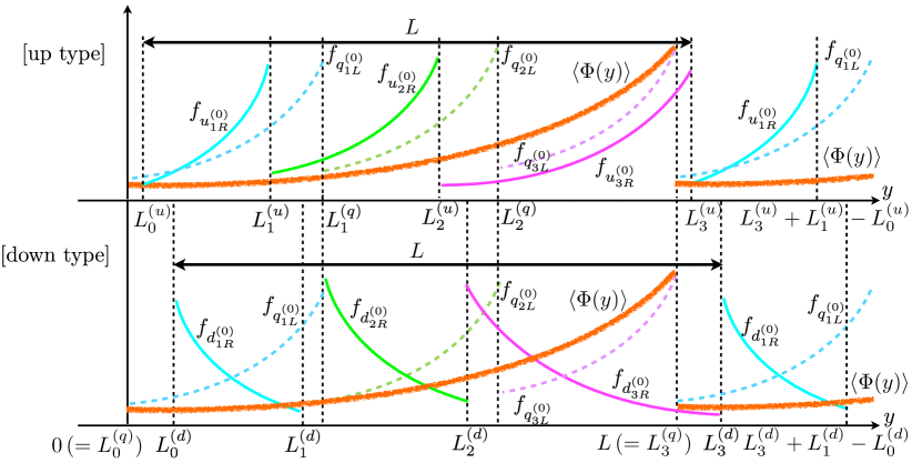
Figure 1: The wave function profiles of the quarks and the VEV of $\Phi(y)$ are schematically depicted. Here we take $L_{0}^{(q)}=L_{0}^{(\Phi)}=0$. Note that all the profiles have the periodicity along $y$ with the same period $L$. Differently from the model on an interval in Ref. [46], we can find the $(1,3)$ elements of the mass matrices due to the periodicity along the $y$ direction.

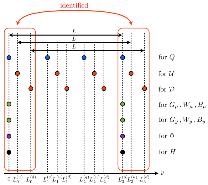
Figure 2: This is an overview of our system with point interactions. The red (blue) circular spots show the Dirichlet BC for left- (right-)handed part at the corresponding boundary points, respectively. The green, purple, and black circular spots represent the ordinary periodic in Eq. (3.19), the Robin BCs in Eq. (3.16), and the twisted BCs in Eq. (2.2), respectively. It is noted that we adopt the assumption in Eq. (4.3).

In the previous section, we introduced the twisted BC for the $SU(2)_{W}$ doublet $H$ and generated the EWSB by the $y$-position-dependent complex VEV in Eq. (2.13) in the case of $M^{2}-(\theta/L)^{2}>0$. We expect that this VEV also works as the source of the $CP$ phase of the CKM matrix, but here an important issue, which we should think about carefully, exists.

If all the profiles of the three-generation quarks are flat, an effective phase appears after integration over $y$ just as an overall factor, which can be removed by $U(1)$ rephasing and never works as a physical $CP$ phase. To circumvent this difficulty, profiles of the quarks are required to be localized. On the other hand, field localization (in extra dimensions) is known as an effective way of explaining the quark mass hierarchy and pattern of flavor mixing. In this section, we consider a model with point interactions as an illustrative example. Point interaction can be considered as zero-thickness brane and we can arrange it anywhere in the bulk space of $S^{1}$.

At the location of a point interaction, we can consider five-dimensional (5D) gauge-invariant boundary conditions, for which the variety is rich compared with the case of $Z_{2}$ orbifolding. After we introduce three point interactions for a 5D fermion, its zero-mode profile gets to be chiral, split and localized. This situation is just what we want. We emphasize that flavor mixing is naturally realized as overlapping of localized quark profiles. In the model, an additional gauge singlet scalar is required for generating the large mass hierarchy of the quarks. Its (almost) exponential shape in the VEV is also generated by a suitable boundary condition at the corresponding point interactions.

This basic idea is found in Ref. [46]. Nevertheless, there are two different points between the models in this paper and in Ref. [46]:

• In the previous model [46], the Higgs VEV cannot possess a nontrivial complex phase, and a $CP$ phase in the CKM matrix has not been realized. On the other hand, the VEV in our present model has a $y$-position-dependent complex phase, which will produce a $CP$ phase of the CKM matrix.

• In the previous model [46], the extra dimension has been taken to be an interval, where the twisted BC in Eq. (2.2) cannot be realized. In the present model, we set the extra dimension to be a circle $S^{1}$, for which the geometry is compatible with the twisted BC (2.2).

In the following part, we briefly explain how to construct our model. The 5D action for fermions is given by

$$S =\int d^{4}x\int_{0}^{L}dy\Bigg{\{}\Big{[}\overline{Q}\left(i\partial_{M}\Gamma^{M}+M_{Q}\right)Q+\overline{\mathcal{U}}\left(i\partial_{M}\Gamma^{M}+M_{\mathcal{U}}\right)\mathcal{U}$$

$$\phantom{=\int d^{4}x\int_{0}^{L_{3}}\Bigg{\{}\ \,}+\overline{\mathcal{D}}\left(i\partial_{M}\Gamma^{M}+M_{\mathcal{D}}\right)\mathcal{D}\Big{]}\Bigg{\}},$$ (3.1)

where we introduce an $SU(2)_{W}$ doublet ($Q$), an up-quark singlet ($\mathcal{U}$), and a down-type singlet ($\mathcal{D}$) with the corresponding bulk masses ($M_{Q},M_{\mathcal{U}},M_{\mathcal{D}}$). We note that our model contains only one generation for 5D quarks but each 5D quark produces three generations of the 4D quarks, as we will see below.

We adopt the following BCs for $Q,\mathcal{U},\mathcal{D}$ with an infinitesimal positive constant $\varepsilon$ [46]:

$$Q_{R} =0\qquad\text{at}\quad y=L_{0}^{(q)}+\varepsilon,\,L_{1}^{(q)}\pm\varepsilon,\,L_{2}^{(q)}\pm\varepsilon,\,L_{3}^{(q)}-\varepsilon,$$ (3.2)

$$\mathcal{U}_{L} =0\qquad\text{at}\quad y=L_{0}^{(u)}+\varepsilon,\,L_{1}^{(u)}\pm\varepsilon,\,L_{2}^{(u)}\pm\varepsilon,\,L_{3}^{(u)}-\varepsilon,$$ (3.3)

$$\mathcal{D}_{L} =0\qquad\text{at}\quad y=L_{0}^{(d)}+\varepsilon,\,L_{1}^{(d)}\pm\varepsilon,\,L_{2}^{(d)}\pm\varepsilon,\,L_{3}^{(d)}-\varepsilon,$$ (3.4)

where $\Psi_{R}$ and $\Psi_{L}$ denote the eigenstates of $\gamma^{5}$, i.e., $\Psi_{R}\equiv\frac{1+\gamma^{5}}{2}\Psi$ and $\Psi_{L}\equiv\frac{1-\gamma^{5}}{2}\Psi$. Here $L^{(i)}_{j}$ for $i=q,u,d$ and $j=0,1,2,3$ means the positions of point interactions for the 5D fermions. See Figs. 1 and 2 for details. A crucial consequence of the above BCs is that there appear threefold degenerated left- (right-)handed zero modes in the mode expansions of $Q$ ($\mathcal{U},\mathcal{D}$) and that they form the three generations of the quarks. The details have been given in Ref. [46]. We will not repeat the discussions here.

The fields $Q,\mathcal{U},\mathcal{D}$ with the BCs in Eqs (3.2)–(3.4) are KK decomposed as follows:

$$Q(x,y)=\begin{pmatrix}U(x,y)\\ D(x,y)\end{pmatrix} =\begin{pmatrix}\sum_{i=1}^{3}u^{(0)}_{iL}(x)f_{q^{(0)}_{iL}}(y)\\ \sum_{i=1}^{3}d^{(0)}_{iL}(x)f_{q^{(0)}_{iL}}(y)\end{pmatrix}+(\text{KK modes}),$$ (3.5)

$$\mathcal{U}(x,y) =\sum_{i=1}^{3}u^{(0)}_{iR}(x)f_{u^{(0)}_{iR}}(y)+(\text{KK modes}),$$ (3.6)

$$\mathcal{D}(x,y) =\sum_{i=1}^{3}d^{(0)}_{iR}(x)f_{d^{(0)}_{iR}}(y)+(\text{KK modes}).$$ (3.7)

Here the zero-mode functions are obtained in the following forms:

$$f_{q^{(0)}_{iL}}(y) =\mathcal{N}_{i}^{(q)}e^{M_{Q}(y-L_{i-1}^{(q)})}\Big{[}\theta(y-L_{i-1}^{(q)})\theta(L_{i}^{(q)}-y)\Big{]} \text{in\ }[L_{0}^{(q)},L_{3}^{(q)}],$$ (3.8)

$$f_{u^{(0)}_{iR}}(y) =\mathcal{N}_{i}^{(u)}e^{-M_{\mathcal{U}}(y-L_{i-1}^{(u)})}\Big{[}\theta(y-L_{i-1}^{(u)})\theta(L_{i}^{(u)}-y)\Big{]} \text{in\ }[L_{0}^{(u)},L_{3}^{(u)}],$$ (3.9)

$$f_{d^{(0)}_{iR}}(y) =\mathcal{N}_{i}^{(d)}e^{-M_{\mathcal{D}}(y-L_{i-1}^{(d)})}\Big{[}\theta(y-L_{i-1}^{(d)})\theta(L_{i}^{(d)}-y)\Big{]} \text{in\ }[L_{0}^{(d)},L_{3}^{(d)}],$$ (3.10)

where

$$\Delta L^{(l)}_{i} =L^{(l)}_{i}-L^{(l)}_{i-1}\qquad(\text{for }i=1,2,3;\ l=q,u,d),$$ (3.11)

$$\mathcal{N}_{i}^{(q)}=\sqrt{\frac{2M_{Q}}{e^{2M_{Q}\Delta L_{i}^{(q)}}-1}},\quad\mathcal{N}_{i}^{(u)}=\sqrt{\frac{2M_{\mathcal{U}}}{1-e^{-2M_{\mathcal{U}}\Delta L_{i}^{(u)}}}},\quad\mathcal{N}_{i}^{(d)}=\sqrt{\frac{2M_{\mathcal{D}}}{1-e^{-2M_{\mathcal{D}}\Delta L_{i}^{(d)}}}}.$$ (3.12)

$\mathcal{N}_{i}^{(q)},\mathcal{N}_{i}^{(u)},\mathcal{N}_{i}^{(d)}$ are the wave function normalization factors for $f_{q^{(0)}_{iL}},f_{u^{(0)}_{iL}},f_{d^{(0)}_{iL}}$, respectively.

Since the length of the total system is universal, $L^{(l)}_{3}-L^{(l)}_{0}\ (l=q,u,d)$ should be equal to the circumference of $S^{1}$, i.e.

$$L:=L^{(q)}_{3}-L^{(q)}_{0}=L^{(u)}_{3}-L^{(u)}_{0}=L^{(d)}_{3}-L^{(d)}_{0}.$$ (3.13)

Note that all the mode functions in Eqs. (3.8)–(3.10) (and a form of a singlet VEV in Eq. (3.17)) are periodic with the common period $L$, whereas we do not indicate that thing explicitly in Eqs. (3.8)–(3.10).

In this model, the large mass hierarchy is naturally explained with the Yukawa sector

$$S_{\mathcal{Y}}=\int d^{4}x\int_{0}^{{L}}dy\bigg{\{}\Phi\Big{[}-\mathcal{Y}^{(u)}\overline{Q}(i\sigma_{2}H^{\ast})\mathcal{U}-\mathcal{Y}^{(d)}\overline{Q}H\mathcal{D}\Big{]}+\text{h.c.}\bigg{\}},$$ (3.14)

where $\mathcal{Y}^{(u)}/\mathcal{Y}^{(d)}$ is the Yukawa coupling for up-/down-type quark; $H$ and $\Phi$ are an $SU(2)_{W}$ scalar doublet and a singlet. It should be noted that although the Yukawa couplings $\mathcal{Y}^{(u)}$ and $\mathcal{Y}^{(d)}$ can be complex, they cannot be an origin of the $CP$ phase of the CKM matrix because our model contains only a single quark generation so that the number of the 5D Yukawa couplings is not enough to produce a $CP$ phase in the CKM matrix. An outline of our system is depicted in Fig. 1. Note that the five terms of $\overline{Q}(i\sigma_{2}H^{\ast})\mathcal{U},\overline{Q}H\mathcal{D},\Phi\overline{Q}Q,\Phi\overline{\mathcal{U}}\mathcal{U},\Phi\overline{\mathcal{D}}\mathcal{D}$ with the Pauli matrix $\sigma_{2}$ are excluded by introducing a discrete symmetry $H\rightarrow-H,\Phi\rightarrow-\Phi$. $\Phi$ is a gauge singlet and there is no problem with gauge universality violation.

The 5D action and the BCs for $\Phi$ are assumed to be of the form [46, 50]

$$S_{\Phi}=\int d^{4}x\int_{0}^{{L}}dy\bigg{\{}{\Phi^{\dagger}\left(\partial_{M}\partial^{M}-{M_{\Phi}}^{2}\right)\Phi-\frac{\lambda_{\Phi}}{2}\left(\Phi^{\dagger}\Phi\right)^{2}}\bigg{\}},$$ (3.15)

$$\Phi+L_{+}\partial_{y}\Phi =0\qquad\text{at}\quad y=L_{0}^{(\Phi)}+\varepsilon,$$

$$\Phi-L_{-}\partial_{y}\Phi =0\qquad\text{at}\quad y=L_{3}^{(\Phi)}-\varepsilon,$$ (3.16)

where $M_{\Phi}$ ($\lambda_{\Phi}$) is the bulk mass (quartic coupling) of the scalar singlet $\Phi$ and $L_{\pm}$ can take values in the range of $-\infty\leq L_{\pm}\leq\infty$ and $L_{0}^{(\Phi)}$ and $L_{3}^{(\Phi)}$ indicate the locations of the two “end points” of the singlet.

The VEV of $\Phi$ with the BCs, named Robin BCs, in Eq. (3.16) is expressed in terms of Jacobi’s elliptic functions in general and its phase structure has been discussed in Ref [50]. We adopt a specific form in the region $[L_{0}^{(\Phi)}+\varepsilon,L_{3}^{(\Phi)}-\varepsilon]$ [46],

$$\left\langle\Phi(y)\right\rangle=\left[{\frac{M_{\Phi}}{\sqrt{\lambda_{\Phi}}}}\left\{\sqrt{1+X}-1\right\}^{1/2}\right]\times\frac{1}{\text{cn}\left({M_{\Phi}}\left\{1+X\right\}^{1/4}(y-y_{0}),\sqrt{\frac{1}{2}\left(1+\frac{1}{\sqrt{1+X}}\right)}\right)},$$ (3.17)

with

$$X:={\frac{4\lambda_{\Phi}|Q|}{M^{4}_{\Phi}}}.$$ (3.18)

Here $y_{0}$ and $Q$ are parameters which appear after integration on $y$ and we focus on the choice of $Q<0$. We note that the values of $y_{0}$ and $Q$ are automatically determined after choosing those of $L_{\pm}$. As shown in Ref. [46], we get the form of $\left\langle\Phi(y)\right\rangle$ to be an (almost) exponential function of $y$ by choosing suitable parameter configurations. Although there is a discontinuity in the wave function profile of $\langle\Phi\rangle$ between $y=L_{0}^{(\Phi)}+\varepsilon$ and $y=L_{3}^{(\Phi)}-\varepsilon$ in Eqs. (3.16), this type of BC is derived from the variational principle on $S^{1}$ and leads to no inconsistency [50].

The BCs for the 5D $SU(3)_{C},SU(2)_{W},U(1)_{Y}$ gauge bosons $G_{M},W_{M},B_{M}$ are selected as

$${G_{M}|_{y=0}=G_{M}|_{y=L},\quad\partial_{y}G_{M}|_{y=0}=\partial_{y}G_{M}|_{y=L},}$$ (3.19)

where we only show the $G_{M}$’s case. In this configuration, we obtain the standard model gauge bosons in zero modes. Based on the discussion in Sec. 2, we conclude that the W and Z bosons become massive and their masses are suitably created through “our” Higgs mechanism as $m_{W}\simeq 81\,\text{GeV},m_{Z}\simeq 90\,\text{GeV}$. The overview of the BCs is summarized in Fig. 2. We mention that, on $S^{1}$ geometry, $G^{(0)}_{y}$, $W^{(0)}_{y}$, and $B^{(0)}_{y}$ would exist as massless 4D scalars at the tree level, but they will become massive via quantum corrections and are expected to be uplifted to near KK states. We will discuss those modes in another paper. We should note that in our model on $S^{1}$ with point interactions, the 5D gauge symmetries are intact under the BCs summarized in Fig. 2. Hence the unitarity in the scattering processes of massive particles are ensured in our model.

4 $CP$ phase in the CKM matrix

In this section, we verify that our mechanism can actually produce a nontrivial $CP$ phase in the CKM matrix. We further would like to find a set of parameter configurations in which the quark mass hierarchy and the structure of the CKM matrix are derived naturally. In the following analysis, we rescale all the dimensional valuables by the $S^{1}$ circumference $L$ to make them dimensionless and the rescaled valuables are indicated with the tilde $\tilde{{}}$ .

We set the parameters concerning the scalar singlet $\Phi$ as

$${\tilde{M}_{\Phi}}=8.67,\quad\tilde{y}_{0}=-0.1,\quad{\tilde{\lambda}_{\Phi}}=0.001,\quad|\tilde{Q}|=0.001,$$ (4.1)

where the VEV profile becomes an (almost) exponential function of $y$, which is suitable for generating the large mass hierarchy. In this case, the values of $L_{\pm}$ in Eq. (3.16) correspond to

$$\frac{1}{\tilde{L}_{+}}=-6.07,\quad\frac{1}{\tilde{L}_{-}}=8.69,$$ (4.2)

where the broken phase is realized [46].

$M_{ij}^{(u)}$	$a$	$b$	$M_{ij}^{(d)}$	$a$	$b$
$M_{11}^{(u)}$	$L_{0}^{(u)}$	$L_{1}^{(u)}$	$M_{11}^{(d)}$	$L_{0}^{(d)}$	$L_{1}^{(d)}$
$M_{22}^{(u)}$	$L_{1}^{(q)}$	$L_{2}^{(u)}$	$M_{22}^{(d)}$	$L_{1}^{(q)}$	$L_{2}^{(d)}$
$M_{33}^{(u)}$	$L_{2}^{(q)}$	$L$	$M_{33}^{(d)}$	$L_{2}^{(q)}$	$L$
$M_{12}^{(u)}$	$L_{1}^{(u)}$	$L_{1}^{(q)}$	$M_{12}^{(d)}$	$L_{1}^{(d)}$	$L_{1}^{(q)}$
$M_{23}^{(u)}$	$L_{2}^{(u)}$	$L_{2}^{(q)}$	$M_{23}^{(d)}$	$L_{2}^{(d)}$	$L_{2}^{(q)}$
$M_{31}^{(u)}$	$L$	$L+L_{0}^{(u)}$	$M_{31}^{(d)}$	$L$	$L+L_{0}^{(d)}$

Table 1: The summary table for the overlap integrals in Eq. (4.6).

As in the previous analysis [46], the signs of the fermion bulk masses are assigned as $M_{Q}>0,M_{\mathcal{U}}<0,M_{\mathcal{D}}>0$ to make much larger overlapping in the up-quark sector than in down ones for top mass. Here we assume the positions of the two end points of both the quark doublet and the scalar singlet are the same

$$L_{0}^{(q)}=L_{0}^{(\Phi)}=0,\quad L_{3}^{(q)}=L_{3}^{(\Phi)}=L,$$ (4.3)

where we set $L_{0}^{(q)}$ and $L_{0}^{(\Phi)}$ as zero. In addition, we also assume that the orders of the positions of point interactions are settled as

$$0<L_{0}^{(u)}<L_{1}^{(u)}<L_{1}^{(q)}<L_{2}^{(u)}<L_{2}^{(q)}<L<L_{3}^{(u)},$$

$$0<L_{0}^{(d)}<L_{1}^{(d)}<L_{1}^{(q)}<L_{2}^{(d)}<L_{2}^{(q)}<L<L_{3}^{(d)}.$$ (4.4)

Here our up-quark mass matrix ${\mathcal{M}}^{(u)}$ and that of down ones ${\mathcal{M}}^{(d)}$ take the forms

$$\mathcal{M}^{(u)}=\begin{bmatrix}M^{(u)}_{11}&M^{(u)}_{12}&M^{(u)}_{13}\\ 0&M^{(u)}_{22}&M^{(u)}_{21}\\ 0&0&M^{(u)}_{33}\end{bmatrix},\quad\mathcal{M}^{(d)}=\begin{bmatrix}M^{(d)}_{11}&M^{(d)}_{12}&M^{(d)}_{13}\\ 0&M^{(d)}_{22}&M^{(d)}_{21}\\ 0&0&M^{(d)}_{33}\end{bmatrix},$$ (4.5)

where the row (column) index of the mass matrices shows the generations of the left- (right-)handed fermions, respectively. Differently from the model on an interval in Ref. [46], the $(1,3)$ elements of the mass matrices are allowed geometrically due to the periodicity along the $y$ direction. The general form of the nonzero matrix elements of ${\mathcal{M}}^{(u)}$ and ${\mathcal{M}}^{(d)}$ can be expressed as

$$M^{(\kappa)}_{ij}={\mathcal{Y}}^{(\kappa)}\int_{a}^{b}\!\!dyf_{q^{(0)}_{iL}}(y)f_{\kappa^{(0)}_{jR}}(y)\langle\Phi(y)\rangle{\langle H(y)\rangle},$$ (4.6)

where $\kappa$ indicates the up/down type of quark and the concrete information is stored in Table 1.

4.1 Quark masses and mixing parameters

The parameters which we use for calculation are

$$\begin{array}[]{llll}\tilde{L}_{0}^{(q)}=0,&\tilde{L}_{1}^{(q)}={0.30},&\tilde{L}_{2}^{(q)}={0.660},&\tilde{L}_{3}^{(q)}=1,\\ \tilde{L}_{0}^{(u)}={0.024},&\tilde{L}_{1}^{(u)}={0.026},&\tilde{L}_{2}^{(u)}={0.52},&\tilde{L}_{3}^{(u)}={1.024},\\ \tilde{L}_{0}^{(d)}={0.07},&\tilde{L}_{1}^{(d)}={0.18},&\tilde{L}_{2}^{(d)}={0.646},&\tilde{L}_{3}^{(d)}={1.07},\\ \tilde{M}_{Q}={6},&\tilde{M}_{\mathcal{U}}={-6},&\tilde{M}_{\mathcal{D}}={5},&\theta={3},\end{array}$$ (4.7)

where the twist angle $\theta$ is a dimensionless value and should be within the range $-\pi<\theta\leq\pi$. We note that $\tilde{L}_{3}^{(q)}$, $\tilde{L}_{3}^{(u)}$, and $\tilde{L}_{3}^{(d)}$ are considered to be not independent degree of freedom, for which the values are automatically determined after we choose the other positions of the point interactions. In Appendix A, we will comment on the orders of significant digits of the input parameters in Eq. (4.7). We should note that in our system, the EWSB is only realized on the condition of ${M}^{2}-\left(\frac{\theta}{L}\right)^{2}>0$ as in Eqs. (2.13). Recently, the ATLAS and CMS experiments have announced that the physical Higgs mass is around $126\,\text{GeV}$ over $5\sigma$ confidence level [62, 63]. $\tilde{\lambda}$ is $0.262$ irrespective of the value of $L$, while $\tilde{M}$ is slightly dependent on the value of $L$ as $3.01303$ $(3.00052)$ in the case of $M_{\text{KK}}=2\,\text{TeV}$ ($M_{\text{KK}}=10\,\text{TeV}$), where $M_{\text{KK}}$ is a typical scale of the KK mode and defined as $2\pi/L$. Here some tuning is required to obtain the suitable values realizing the EWSB.

After the diagonalization of the two mass matrices, the quark masses are evaluated as

$$\begin{array}[]{lll}m_{\text{up}}={2.5}\,\text{MeV},&m_{\text{charm}}={1.339}\,\text{GeV},&m_{\text{top}}={173.3}\,\text{GeV},\\ m_{\text{down}}={4.8}\,\text{MeV},&m_{\text{strange}}={104}\,\text{MeV},&m_{\text{bottom}}={4.183}\,\text{GeV},\\ \vspace{-4mm}\\ \displaystyle\frac{m_{\text{up}}}{m_{\text{up}}|_{\text{exp.}}}={1.07},&\displaystyle\frac{m_{\text{charm}}}{m_{\text{charm}}|_{\text{exp.}}}={1.05},&\displaystyle\frac{m_{\text{top}}}{m_{\text{top}}|_{\text{exp.}}}=1.00,\\ \vspace{-4mm}\\ \displaystyle\frac{m_{\text{down}}}{m_{\text{down}}|_{\text{exp.}}}={0.993},&\displaystyle\frac{m_{\text{strange}}}{m_{\text{strange}}|_{\text{exp.}}}={1.10},&\displaystyle\frac{m_{\text{bottom}}}{m_{\text{bottom}}|_{\text{exp.}}}=1.00,\end{array}$$ (4.8)

and the absolute values of the CKM matrix elements are given as

$$|V_{\text{CKM}}|=\begin{bmatrix}{0.971}&{0.238}&{0.00377}\\ {0.237}&{0.971}&{0.0403}\\ {0.00887}&{0.0395}&0.999\end{bmatrix},\quad\left|\frac{V_{\text{CKM}}}{V_{\text{CKM}}|_{\text{exp.}}}\right|=\begin{bmatrix}0.997&1.06&{1.07}\\ 1.06&0.998&{0.978}\\ {1.02}&{0.978}&1.00\end{bmatrix}.$$ (4.9)

4.2 $CP$ phase

The Jarlskog parameter $J$ containing information about the $CP$ phase is defined by

$$\text{Im}\left[(V_{\text{CKM}})_{ij}(V_{\text{CKM}})_{kl}(V_{\text{CKM}}^{\ast})_{il}(V_{\text{CKM}}^{\ast})_{kj}\right]=J\sum_{m,n=1}^{3}\epsilon_{ikm}\epsilon_{jln}$$ (4.10)

with the completely antisymmetric tensor $\epsilon$, and is invariant under the $U(1)$ unphysical rephasing operations of six types of quarks [64, 65]. This value is easily estimated as

$$J={3.23}\times 10^{-5},\quad\frac{J}{J|_{\text{exp.}}}={1.09},$$ (4.11)

where we also provide the differences from the latest experimental values in Ref. [66]. All the deviations from the latest experimental values are within about $10\%$, and we can conclude that the situation of the SM is suitably generated. In Appendix A, we discuss distribution patterns of quark mass-matrix elements and required orders in tuning the input parameters with the results for realizing the accuracy.

5 Summary and discussion

In this paper, we have proposed a new mechanism for generating a $CP$ phase via a Higgs VEV originating from the geometry of an extra dimension. A twisted BC for the Higgs doublet has been found to lead to an extra-dimension coordinate-dependent phase in the Higgs VEV, which contains a nontrivial $CP$ phase degree of freedom. This mechanism is useful for generating a $CP$ phase to a single generation extra-dimensional field theory incorporating with a generation production mechanism. The electroweak symmetry breaking is also generated dynamically due to the twisted boundary condition with the suitable W- and Z-boson masses.

As an illustrative example, we applied our mechanism to a five-dimensional gauge theory on a circle with point interactions [46]. Point interactions, which are additional boundary points with respect to the extra dimension, are responsible for producing the three generations while the model consists of a single-generation fermion and make the quark profiles be localized. Since each element of the mass matrices picks up a different phase through the overlap integrals, there is some possibility of realizing a nontrivial $CP$ phase. After numerical calculations, we found that a nontrivial $CP$ phase appears with good precision, maintaining the property of the original model in which the generations, the quark mass hierarchy and the CKM matrix appear from the geometry of the extra dimension. Certainly, our new mechanism for generating a $CP$ phase via Higgs VEV works.

A key point of our mechanism is that we can generate both the EWSB and a $CP$ phase simultaneously as a complex Higgs VEV. To make our $CP$-violation mechanism work correctly, quark profiles should be split and localized. In this situation, flavor mixing and mass hierarchy of the quarks are also naturally activated. We would like to emphasize that in the model adopting our mechanism, all the concepts of quark flavor in the SM, namely EWSB, the number of generations, flavor mixing, mass hierarchy, and $CP$ violation, are interlinked closely.

One of the most important remaining tasks is to construct a model which brings both the quarks and the leptons into perspective. Using our mechanism, not only the quark sector but also the lepton sector can acquire a nontrivial $CP$ phase. Since the origin of the $CP$ phase is common, we can predict the value of the $CP$ phase of the lepton sector after fitting the value of the $CP$ phase in the quark sector. The result will be reported elsewhere. Accommodation of our mechanism to another single generation model is also an important task.

Another crucial topic is the stability of the system. Our system is possibly threatened with instability. Some mechanisms will be required to stabilize the moduli representing the positions of point interactions (branes). In a multiply connected space of $S^{1}$, there is another origin of gauge symmetry breaking, i.e., the Hosotani mechanism [70, 71]. Since further gauge symmetry breaking causes a problem in the model, we need to insure that the Hosotani mechanism does not occur. To this end, we might introduce additional 5D matter to prevent zero modes of $y$ components of gauge fields from acquiring nonvanishing VEVs. We will leave those issues in future work.

Appendix

Appendix A Considering input-parameter dependence

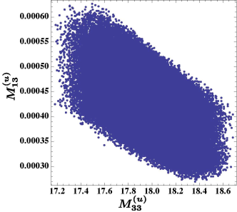
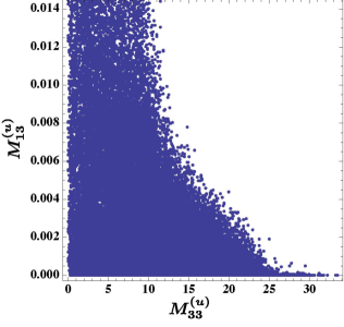
Figure 3: The left scatter plot shows the distribution of $M_{33}^{(u)}-M_{13}^{(u)}$ when we choose 100,000 points randomly around the configuration in Eq.(4.7) within $\pm 10\%$ being consistent with the order in Eq. (4.4). The right one represents the same thing when we pick up 100,000 points randomly only with following the order in Eq. (4.4).

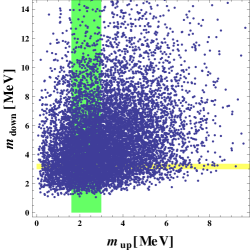
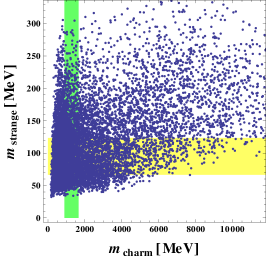
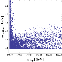
Figure 4: From left to right, distributions of $m_{\text{up}}-m_{\text{down}}$, $m_{\text{charm}}-m_{\text{strange}}$ and $m_{\text{top}}-m_{\text{bottom}}$ with 10,000 random points within $\pm 20\%$ parameter deviations from the central values in Eq. (4.7 following the order in Eq. (4.4). The green (yellow) band in the left and center plots represents $\pm 30\%$ range from the central values in Eq. (4.7). In the right plot, we skip depicting the bands because all the shown ranges are covered by them.

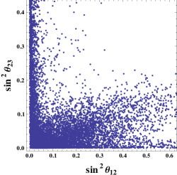
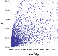
Figure 5: From left to right, distributions of $\sin^{2}{\theta_{12}}-\sin^{2}{\theta_{23}}$ and $\sin^{2}{\theta_{13}}-J$ with 10,000 random points within $\pm 20\%$ parameter deviations from the central values in Eq. (4.7) following the order in Eq. (4.4). The allowed region is just near the point $(0,0)$ in both the plots.

In this appendix, we discuss distribution patterns of quark mass-matrix elements and required orders in tuning the input parameters with the results given in Sec. 4.1 and 4.2.

We first focus on the matrices in Eq. (4.5). In our model, the geometry of the extra dimension strongly restricts the form of the matrices. In fact, we cannot fill all the elements of the mass matrices and at least three of the nine elements for each mass matrix have to be zero, as shown in Eq. (4.5). This property is contrasted with that of the standard model, where all the mass matrix elements are free parameters. This fact means that possible patterns of mass matrices are constrained by the shape of the geometry of our model.

Furthermore, it turns out that the values of the nonzero elements in the mass matrices (4.5) cannot be controlled freely. To see this, we investigated correlations of matrix elements. In the left figure of Fig. 3, we chose 100,000 points randomly around the configuration in Eq.(4.7) within $\pm 10\%$ being consistent with the order in Eq. (4.4) and depicted the resultant values as two scatter plots ($M_{33}^{(u)}-M_{13}^{(u)}$). The right figure of Fig. 3 shows the same thing when we pick up 100,000 points randomly only with following the order in Eq. (4.4).

It follows from Fig. 3 that we find no random distribution in the $M^{(u)}_{33}-M^{(u)}_{13}$ plane and a strong correlation between $M^{(u)}_{13}$ and $M^{(u)}_{33}$. We further see the property that the typical value of $M^{(u)}_{13}$ is much smaller than that of $M^{(u)}_{33}$. In the quark sector, the mixing angles are known to be small, so that off-diagonal elements of the mass matrices will be preferred to be subleading compared with the diagonal ones with suitable magnitudes. Our geometry realizes this point naturally via its geometry.

From the above observations, we may conclude that the quark mass matrices in our model are considerably restricted from the geometry of the extra dimension, and hence that it is nontrivial to reproduce the quark-related properties of the standard model, although we have 16 input parameters for quark profiles, where 13 parameters are independent, to explain the 10 standard model parameters (6 quarks masses and 4 CKM parameters).

As another consideration, we investigate the resultant quark masses and CKM matrix elements when we change the input parameters around the central values in Eq. (4.7) and then find that the quark masses and CKM matrix elements are very sensitive to some of the input parameters.

To show the sensitivity of the input parameters, we first alter all the parameters randomly within $10\%$, $1\%$, $0.1\%$, and $0.01\%$, respectively, obeying the order in Eq. (4.4), and calculate the masses and the elements. When we proceed with the above procedure 100,000 times in each case, 11, 11,039, 81,955, and 100,000 points survive after putting the cut where all the resultants are within $15\%$. These results indicate that parameter tuning less than $1\%$ is required as our inputs are so in Eq. (4.7). The scatter plots in Figs. 4 and 5 represent the distributions of the physical parameters with 10,000 random points within $\pm 20\%$ around the central values, where the CKM angles and the Jarlskog parameter are apt to getting away from the required range easily, for which the experimental central values are $\sin^{2}{\theta_{12}}\sim 0.05$, $\sin^{2}{\theta_{23}}\sim 0.002$, $\sin^{2}{\theta_{13}}\sim 0.00001$, and $J\sim 0.00003$, respectively. This issue is explained by the fact that off-diagonal elements of the CKM matrix are closely related to those of the up- and down-quark mass matrices, which at least parts of them are, sensitive to perturbation of the input parameters. We can also find the tendency that bottom and top masses are not away from the central values by the perturbation.

On the other hand, we try to alter an input parameter separately. In each case, points of the numbers in Table 2 pass the cut which rejects the possibilities that at least one resultant value is out of the $\pm 15\%$ deviation range from the central value in Eq. (4.7). According to the result, we understand that quark masses and mixing angles are sensitive to the positions of point interactions, while those are insensitive to (absolute values of) the bulk masses and the twisted angle. Then we can conclude that parameter tuning in $M_{Q}$, $M_{\mathcal{U}}$, $M_{\mathcal{D}}$, and $\theta$ in Eq. (4.7) is not always necessary.

Finally, we briefly comment on the required orders of significant digits in the input parameters. As we have discussed before based on Table 2, the system is insensitive to $M_{Q}$, $M_{\mathcal{U}}$, $M_{\mathcal{D}}$, and $\theta$ around the central region of the parameters, and then single digits are sufficient for them. On the other hand, for $L_{2}^{(q)}$ and $L_{2}^{(d)}$, as also expressed in Table 2, triple digits are required because of their great sensitivity. For the other values, tuning up to double digits is enough for our purpose since they are less sensitive than $L_{2}^{(q)}$ and $L_{2}^{(d)}$ as shown in Table 2.

parameter	$L_{1}^{(q)}$	$L_{2}^{(q)}$	$L_{0}^{(u)}$	$L_{1}^{(u)}$	$L_{2}^{(u)}$	$L_{0}^{(d)}$	$L_{1}^{(d)}$	$L_{2}^{(d)}$	$M_{Q}$	$M_{\mathcal{U}}$	$M_{\mathcal{D}}$	$\theta$
$\#$ of surviving points	105	11	46	85	42	270	172	10	679	730	372	971

Table 2: Numbers of surviving points out of 1,000 ones after the cut where all the physical resultants are within $\pm 15\%$ with changing an input parameter within $\pm 10\%$ from the central values in Eq. (4.7) individually.

References

- [1] M. Kobayashi and T. Maskawa, “CP Violation in the Renormalizable Theory of Weak Interaction,” Prog.Theor.Phys. 49 (1973) 652–657.
- [2] N. Arkani-Hamed, S. Dimopoulos, G. R. Dvali, and J. March-Russell, “Neutrino masses from large extra dimensions,” Phys.Rev. D65 (2001) 024032, arXiv:hep-ph/9811448 [hep-ph].
- [3] N. Arkani-Hamed and M. Schmaltz, “Hierarchies without symmetries from extra dimensions,” Phys.Rev. D61 (2000) 033005, arXiv:hep-ph/9903417 [hep-ph].
- [4] G. Dvali and A. Y. Smirnov, “Probing large extra dimensions with neutrinos,” Nucl.Phys. B563 (1999) 63–81, arXiv:hep-ph/9904211 [hep-ph].
- [5] K. Yoshioka, “On fermion mass hierarchy with extra dimensions,” Mod.Phys.Lett. A15 (2000) 29–40, arXiv:hep-ph/9904433 [hep-ph].
- [6] R. Mohapatra, S. Nandi, and A. Perez-Lorenzana, “Neutrino masses and oscillations in models with large extra dimensions,” Phys.Lett. B466 (1999) 115–121, arXiv:hep-ph/9907520 [hep-ph].
- [7] Y. Grossman and M. Neubert, “Neutrino masses and mixings in nonfactorizable geometry,” Phys.Lett. B474 (2000) 361–371, arXiv:hep-ph/9912408 [hep-ph].
- [8] G. R. Dvali and M. A. Shifman, “Families as neighbors in extra dimension,” Phys.Lett. B475 (2000) 295–302, arXiv:hep-ph/0001072 [hep-ph].
- [9] T. Gherghetta and A. Pomarol, “Bulk fields and supersymmetry in a slice of AdS,” Nucl.Phys. B586 (2000) 141–162, arXiv:hep-ph/0003129 [hep-ph].
- [10] S. J. Huber and Q. Shafi, “Fermion masses, mixings and proton decay in a Randall-Sundrum model,” Phys.Lett. B498 (2001) 256–262, arXiv:hep-ph/0010195 [hep-ph].
- [11] M. V. Libanov and S. V. Troitsky, “Three fermionic generations on a topological defect in extra dimensions,” Nucl.Phys. B599 (2001) 319–333, arXiv:hep-ph/0011095 [hep-ph].
- [12] J. M. Frere, M. V. Libanov, and S. V. Troitsky, “Three generations on a local vortex in extra dimensions,” Phys.Lett. B512 (2001) 169–173, arXiv:hep-ph/0012306 [hep-ph].
- [13] A. Neronov, “Fermion masses and quantum numbers from extra dimensions,” Phys.Rev. D65 (2002) 044004, arXiv:gr-qc/0106092 [gr-qc].
- [14] J. M. Frere, M. V. Libanov, and S. V. Troitsky, “Neutrino masses with a single generation in the bulk,” JHEP 0111 (2001) 025, arXiv:hep-ph/0110045 [hep-ph].
- [15] D. E. Kaplan and T. M. P. Tait, “New tools for fermion masses from extra dimensions,” JHEP 0111 (2001) 051, arXiv:hep-ph/0110126 [hep-ph].
- [16] S. L. Parameswaran, S. Randjbar-Daemi, and A. Salvio, “Gauge Fields, Fermions and Mass Gaps in 6D Brane Worlds,” Nucl.Phys. B767 (2007) 54–81, arXiv:hep-th/0608074 [hep-th].
- [17] M. Gogberashvili, P. Midodashvili, and D. Singleton, “Fermion Generations from ’Apple-Shaped’ Extra Dimensions,” JHEP 0708 (2007) 033, arXiv:0706.0676 [hep-th].
- [18] D. B. Kaplan and S. Sun, “Spacetime as a topological insulator: Mechanism for the origin of the fermion generations,” Phys.Rev.Lett. 108 (2012) 181807, arXiv:1112.0302 [hep-ph].
- [19] G. Burdman and Y. Nomura, “Unification of Higgs and gauge fields in five-dimensions,” Nucl.Phys. B656 (2003) 3–22, arXiv:hep-ph/0210257 [hep-ph].
- [20] Y. Adachi, N. Kurahashi, N. Maru, and K. Tanabe, “CP Violation due to Flavor Mixing in Gauge-Higgs Unification,” arXiv:1201.2290 [hep-ph].
- [21] C. S. Lim, N. Maru, and K. Nishiwaki, “CP Violation due to Compactification,” Phys.Rev. D81 (2010) 076006, arXiv:0910.2314 [hep-ph].
- [22] M. Sakamoto, M. Tachibana, and K. Takenaga, “Spontaneously broken translational invariance of compactified space,” Phys.Lett. B457 (1999) 33–38, arXiv:hep-th/9902069 [hep-th].
- [23] M. Sakamoto, M. Tachibana, and K. Takenaga, “Spontaneous supersymmetry breaking from extra dimensions,” Phys.Lett. B458 (1999) 231–236, arXiv:hep-th/9902070 [hep-th].
- [24] M. Sakamoto, M. Tachibana, and K. Takenaga, “A New mechanism of spontaneous SUSY breaking,” Prog.Theor.Phys. 104 (2000) 633–676, arXiv:hep-th/9912229 [hep-th].
- [25] K. Ohnishi and M. Sakamoto, “Novel phase structure of twisted model on ,” Phys.Lett. B486 (2000) 179–185, arXiv:hep-th/0005017 [hep-th].
- [26] H. Hatanaka, S. Matsumoto, K. Ohnishi, and M. Sakamoto, “Vacuum structure of twisted scalar field theories on ,” Phys.Rev. D63 (2001) 105003, arXiv:hep-th/0010283 [hep-th].
- [27] S. Matsumoto, M. Sakamoto, and S. Tanimura, “Spontaneous breaking of the rotational symmetry induced by monopoles in extra dimensions,” Phys.Lett. B518 (2001) 163–170, arXiv:hep-th/0105196 [hep-th].
- [28] M. Sakamoto and S. Tanimura, “Spontaneous breaking of the C, P, and rotational symmetries by topological defects in extra two dimensions,” Phys.Rev. D65 (2002) 065004, arXiv:hep-th/0108208 [hep-th].
- [29] F. Coradeschi, S. De Curtis, D. Dominici, and J. R. Pelaez, “Modified spontaneous symmetry breaking pattern by brane-bulk interaction terms,” JHEP 0804 (2008) 048, arXiv:0712.0537 [hep-th].
- [30] C. Burgess, C. de Rham, and L. van Nierop, “The Hierarchy Problem and the Self-Localized Higgs,” JHEP 0808 (2008) 061, arXiv:0802.4221 [hep-ph].
- [31] N. Haba, K.-y. Oda, and R. Takahashi, “Top Yukawa Deviation in Extra Dimension,” Nucl.Phys. B821 (2009) 74–128, arXiv:0904.3813 [hep-ph].
- [32] H. Hatanaka, M. Sakamoto, M. Tachibana, and K. Takenaga, “Many brane extension of the Randall-Sundrum solution,” Prog.Theor.Phys. 102 (1999) 1213–1218, arXiv:hep-th/9909076 [hep-th].
- [33] T. Nagasawa, M. Sakamoto, and K. Takenaga, “Supersymmetry in quantum mechanics with point interactions,” Phys.Lett. B562 (2003) 358–364, arXiv:hep-th/0212192 [hep-th].
- [34] T. Nagasawa, M. Sakamoto, and K. Takenaga, “Supersymmetry and discrete transformations on with point singularities,” Phys.Lett. B583 (2004) 357–363, arXiv:hep-th/0311043 [hep-th].
- [35] T. Nagasawa, M. Sakamoto, and K. Takenaga, “Extended supersymmetry and its reduction on a circle with point singularities,” J.Phys. A38 (2005) 8053–8082, arXiv:hep-th/0505132 [hep-th].
- [36] T. Nagasawa, S. Ohya, K. Sakamoto, M. Sakamoto, and K. Sekiya, “Hierarchy of QM SUSYs on a Bounded Domain,” J.Phys. A42 (2009) 265203, arXiv:0812.4659 [hep-th].
- [37] T. Flacke, A. Menon, and D. J. Phalen, “Non-minimal universal extra dimensions,” Phys.Rev. D79 (2009) 056009, arXiv:0811.1598 [hep-ph].
- [38] A. Datta, U. K. Dey, A. Shaw, and A. Raychaudhuri, “Universal Extra-Dimensional models with boundary localized kinetic terms: Probing at the LHC,” arXiv:1205.4334 [hep-ph].
- [39] A. Datta, K. Nishiwaki, and S. Niyogi, “Non-minimal Universal Extra Dimensions: The strongly interacting sector at the Large Hadron Collider,” JHEP 1211 (2012) 154, arXiv:1206.3987 [hep-ph].
- [40] T. Flacke, A. Menon, and Z. Sullivan, “Constraints on UED from W’ searches,” Phys.Rev. D86 (2012) 093006, arXiv:1207.4472 [hep-ph].
- [41] F. J. Petriello, “Kaluza-Klein effects on Higgs physics in universal extra dimensions,” JHEP 0205 (2002) 003, arXiv:hep-ph/0204067 [hep-ph].
- [42] K. Nishiwaki, “Higgs production and decay processes via loop diagrams in various 6D Universal Extra Dimension Models at LHC,” JHEP 1205 (2012) 111, arXiv:1101.0649 [hep-ph].
- [43] K. Nishiwaki, K.-y. Oda, N. Okuda, and R. Watanabe, “A bound on Universal Extra Dimension Models from up to of LHC Data at 7TeV,” Phys.Lett. B707 (2012) 506–511, arXiv:1108.1764 [hep-ph].
- [44] T. Kakuda, K. Nishiwaki, K.-y. Oda, N. Okuda, and R. Watanabe, “Higgs at ILC in Universal Extra Dimensions in Light of Recent LHC Data,” arXiv:1202.6231 [hep-ph].
- [45] G. Belanger, A. Belyaev, M. Brown, M. Kakizaki, and A. Pukhov, “Testing Minimal Universal Extra Dimensions Using Higgs Boson Searches at the LHC,” Phys.Rev. D87 (2013) 016008, arXiv:1207.0798 [hep-ph].
- [46] Y. Fujimoto, T. Nagasawa, K. Nishiwaki, and M. Sakamoto, “Quark mass hierarchy and mixing via geometry of extra dimension with point interactions,” PTEP 2013 (2013) 023B07, arXiv:1209.5150 [hep-ph].
- [47] D. Cremades, L. Ibanez, and F. Marchesano, “Computing Yukawa couplings from magnetized extra dimensions,” JHEP 0405 (2004) 079, arXiv:hep-th/0404229 [hep-th].
- [48] Y. Fujimoto, T. Kobayashi, T. Miura, K. Nishiwaki, and M. Sakamoto, “Shifted orbifold models with magnetic flux,” Phys.Rev. D87 (2013) 086001, arXiv:1302.5768 [hep-th].
- [49] T.-h. Abe, Y. Fujimoto, T. Kobayashi, T. Miura, K. Nishiwaki, et al., “ twisted orbifold models with magnetic flux,” arXiv:1309.4925 [hep-th].
- [50] Y. Fujimoto, T. Nagasawa, S. Ohya, and M. Sakamoto, “Phase Structure of Gauge Theories on an Interval,” Prog.Theor.Phys. 126 (2011) 841–854, arXiv:1108.1976 [hep-th].
- [51] C. S. Lim, T. Nagasawa, M. Sakamoto, and H. Sonoda, “Supersymmetry in gauge theories with extra dimensions,” Phys.Rev. D72 (2005) 064006, arXiv:hep-th/0502022 [hep-th].
- [52] C. S. Lim, T. Nagasawa, S. Ohya, K. Sakamoto, and M. Sakamoto, “Supersymmetry in 5d gravity,” Phys.Rev. D77 (2008) 045020, arXiv:0710.0170 [hep-th].
- [53] C. S. Lim, T. Nagasawa, S. Ohya, K. Sakamoto, and M. Sakamoto, “Gauge-Fixing and Residual Symmetries in Gauge/Gravity Theories with Extra Dimensions,” Phys.Rev. D77 (2008) 065009, arXiv:0801.0845 [hep-th].
- [54] R. S. Chivukula, D. A. Dicus, and H.-J. He, “Unitarity of compactified five-dimensional Yang-Mills theory,” Phys.Lett. B525 (2002) 175–182, arXiv:hep-ph/0111016 [hep-ph].
- [55] Y. Abe, N. Haba, Y. Higashide, K. Kobayashi, and M. Matsunaga, “Unitarity in gauge symmetry breaking on orbifold,” Prog.Theor.Phys. 109 (2003) 831–842, arXiv:hep-th/0302115 [hep-th].
- [56] R. S. Chivukula, D. A. Dicus, H.-J. He, and S. Nandi, “Unitarity of the higher dimensional standard model,” Phys.Lett. B562 (2003) 109–117, arXiv:hep-ph/0302263 [hep-ph].
- [57] C. Csaki, C. Grojean, H. Murayama, L. Pilo, and J. Terning, “Gauge theories on an interval: Unitarity without a Higgs boson,” Phys.Rev. D69 (2004) 055006, arXiv:hep-ph/0305237 [hep-ph].
- [58] T. Ohl and C. Schwinn, “Unitarity, BRST symmetry and ward identities in orbifold gauge theories,” Phys.Rev. D70 (2004) 045019, arXiv:hep-ph/0312263 [hep-ph].
- [59] Y. Abe, N. Haba, K. Hayakawa, Y. Matsumoto, M. Matsunaga, et al., “4-D equivalence theorem and gauge symmetry on orbifold,” Prog.Theor.Phys. 113 (2005) 199–213, arXiv:hep-th/0402146 [hep-th].
- [60] N. Sakai and N. Uekusa, “Selecting gauge theories on an interval by 5D gauge transformations,” Prog.Theor.Phys. 118 (2007) 315–335, arXiv:hep-th/0604121 [hep-th].
- [61] K. Nishiwaki and K.-y. Oda, “Unitarity in Dirichlet Higgs Model,” Eur.Phys.J. C71 (2011) 1786, arXiv:1011.0405 [hep-ph].
- [62] ATLAS Collaboration, G. Aad et al., “Observation of a new particle in the search for the Standard Model Higgs boson with the ATLAS detector at the LHC,” Phys.Lett. B716 (2012) 1–29, arXiv:1207.7214 [hep-ex].
- [63] CMS Collaboration, S. Chatrchyan et al., “Observation of a new boson at a mass of 125 GeV with the CMS experiment at the LHC,” Phys.Lett. B716 (2012) 30–61, arXiv:1207.7235 [hep-ex].
- [64] C. Jarlskog, “Commutator of the Quark Mass Matrices in the Standard Electroweak Model and a Measure of Maximal CP Nonconservation,” Phys.Rev.Lett. 55 (1985) 1039.
- [65] C. Jarlskog, “A Basis Independent Formulation of the Connection Between Quark Mass Matrices, CP Violation and Experiment,” Z.Phys. C29 (1985) 491–497.
- [66] Particle Data Group Collaboration, J. Beringer et al., “Review of Particle Physics (RPP),” Phys.Rev. D86 (2012) 010001.
- [67] L. C. de Albuquerque and R. M. Cavalcanti, “Casimir effect for the scalar field under Robin boundary conditions: A Functional integral approach,” J.Phys. A37 (2004) 7039–7050, arXiv:hep-th/0311052 [hep-th].
- [68] Z. Bajnok, L. Palla, and G. Takacs, “Casimir force between planes as a boundary finite size effect,” Phys.Rev. D73 (2006) 065001, arXiv:hep-th/0506089 [hep-th].
- [69] M. Pawellek, “Quantum mass correction for the twisted kink,” J.Math.Phys. 42 (2009) 045404, arXiv:0802.0710 [hep-th].
- [70] Y. Hosotani, “Dynamical Mass Generation by Compact Extra Dimensions,” Phys.Lett. B126 (1983) 309.
- [71] Y. Hosotani, “Dynamics of Nonintegrable Phases and Gauge Symmetry Breaking,” Annals Phys. 190 (1989) 233.