Dimer XXZ Spin Ladders: Phase diagram and a Non-Trivial Antiferromagnetic Phase

Abstract

We study the dimer $XXZ$ spin model on two-leg ladders with isotropic Heisenberg interactions on the rung and anisotropic $XXZ$ interactions along the rail in an external field. Combining both analytical and numerical methods, we set up the ground state phase diagram and investigate the quantum phase transitions and the properties of rich phases, including the full polarized, singlet dimer, Luttinger liquid, triplon solid, and a non-trivial antiferromagnetic phases with gap. The analytical analyses based on solvable effective Hamiltonians are presented for clear view of the phases and transitions. Quantum Monte Carlo and exact diagonalization methods are employed on finite system to verify the exact nature of the phases and transitions. Of all the phases, we pay a special attention to the gapped antiferromagnetic phase, which is disclosed to be a non-trivial one that exhibits the time-reversal symmetry. We also discuss how our findings could be detected in experiment in the light of ultracold atoms technology advances.

1 Introduction

Ladders (or ladders-like) systems are of great interest in condensed matter physics. On one hand, spin ladders materials with intriguing magnetic properties have been found or synthesized [1, 2]. On the other hand, due to the advances of cold atom technology, optical ladders might be provided as one of the simplest accessible objects that exhibit fascinating properties of quantum matters [3, 4, 5, 8, 7, 9, 6, 10]. Apparently, real compounds are not so flexible as the cold atoms in optical lattices in exploring the underlying mechanism of theoretical models. Progresses in these two fields could interplay and lead to a promising boom of new findings.

In this work, we investigate a two-leg spin ladders in the strong anisotropic limit. We construct the ground state phase diagram and investigate the properties of rich phases, including the full polarized (FP), singlet dimer (SD), Luttinger liquid (LL), triplon solid (TS), and non-trivial antiferromagnet (non-trivial AF) ones. We set up the low-energy effective models for describing different phases within the frame of bond operator theory. Numerical methods including exact diagonalization (ED) and quantum Monte Carlo (QMC) are employed to verify our new findings. We also discuss how our interesting results could be related to experiment.

2 The model

The model we are concerned with is the dimer $XXZ$ spin-1/2 model on two-leg ladders

$$H = \sum_{j}\sum_{l=1,2}\left[J^{x}\left(S_{l,j}^{x}S_{l,j+1}^{x}+S_{l,j}^{y}S_{l,j+1}^{y}\right)+J^{z}S_{l,j}^{z}S_{l,j+1}^{z}-hS_{l,j}^{z}\right]$$ (1)

$$+\sum_{j}K\mathbf{S}_{1,j}\cdot\mathbf{S}_{2,j}.$$

where $S_{l,j}^{\alpha}$ denotes the $S=1/2$ spin operator of $\alpha$ ($\alpha=x,y,z$) component at site $j$ ($j=1,2,...,L$) of $l$-th ($l=1,2$) leg. $J^{x},J^{z}$ are the interactions strength along rail in transverse and longitude directions respectively, $K$ is the Heisenberg interaction strength along rung and will be set as the energy unit, $h$ denotes the Zeeman field. For convenience, we consider the case of $J^{x}>0$ and $J^{z}>0$, and a bipartite lattice without frustration, i.e. $L$ is even when periodic boundary condition is imposed. We will focus on the strong anisotropic cases, e.g. $J^{x}\rightarrow 0$ and $J^{z}\neq 0$, which are not readily to be found in real compounds. Recent progress in the technology of cold atoms are encouraging [9]. The above model can be translated to an identical hardcore bosonic $t$-$V$ model by a Matsubara-Matsuda mapping [11]. Although some experiment on hardcore bosons have been realized [12], but the interaction terms in this model need more sophisticated methods to realize [5, 9]. One may consider a ladder-shaped optical lattice formed by standing wave lasers [13]. The superexchange mechanism could be mimicked by controlled tunneling of cold bosonic or fermionic atoms with two internal states, such as ⁸⁷Rb in $|\uparrow\rangle=b_{\uparrow}^{{\dagger}}|0\rangle=|F=1,m_{F}=1\rangle$ or $|\downarrow\rangle=b_{\downarrow}^{{\dagger}}|0\rangle=|F=1,m_{F}=-1\rangle$, where $|0\rangle$ is a vacuum. So that we can define a spin on a site in a bilinear form $S^{\alpha}=\frac{1}{2}b^{{\dagger}}\sigma^{\alpha}b$, where $\sigma^{\alpha},(\alpha=x,y,z)$, is a pauli matrix and $b^{{\dagger}}=(b_{\uparrow}^{{\dagger}},b_{\downarrow}^{{\dagger}})$. In the Mott insulating phase, the above model could be realized with almost arbitrary model parameters [8, 9].

Before solving the model, we introduce a bond operator representation that will be very useful for elaborating the phenomena we found in this system. There are four states on each rung, one singlet and three triplets,

$$|s\rangle_{j} = \frac{1}{\sqrt{2}}(|\uparrow\downarrow\rangle_{j}-\left|\downarrow\uparrow\right\rangle_{j}),$$

$$|t_{+}\rangle_{j} = |\uparrow\uparrow\rangle_{j},$$

$$|t_{0}\rangle_{j} = \frac{1}{\sqrt{2}}(|\uparrow\downarrow\rangle_{j}+\left|\downarrow\uparrow\right\rangle_{j}),$$

$$|t_{-}\rangle_{j} = |\downarrow\downarrow\rangle_{j}.$$

It is natural to introduce the bond operators $s_{j}^{{\dagger}}$, $t_{+,j}^{{\dagger}}$, $t_{0,j}^{{\dagger}}$, $t_{-,j}^{{\dagger}}$, which create the singlet state and triplet states at $j$-th rung with the constraint, $s_{j}^{{\dagger}}s_{j}+t_{+,j}^{{\dagger}}t_{+,j}+t_{0,j}^{{\dagger}}t_{0,j}+t_{-,j}^{{\dagger}}t_{-,j}=1$. Then the original Hamiltonian Eq.(1) can be rewritten in terms of these bond operators as

$$H = \frac{K}{4}\sum_{j}(-3s_{j}^{{\dagger}}s_{j}+t_{+,j}^{{\dagger}}t_{+,j}+t_{0,j}^{{\dagger}}t_{0,j}+t_{-,j}^{{\dagger}}t_{-,j})+$$ (2)

$$\frac{J^{x}}{2}\sum_{j}[-s_{j}^{{\dagger}}s_{j+1}^{{\dagger}}(t_{+,j}t_{-,j+1}+t_{-,j}t_{+,j+1})+s_{j}^{{\dagger}}s_{j+1}(t_{+,j}t_{+,j+1}^{{\dagger}}+t_{-,j}t_{-,j+1}^{{\dagger}})+$$

$$t_{0,j}t_{0,j+1}(t_{+,j}^{{\dagger}}t_{-,j+1}^{{\dagger}}+t_{-,j}^{{\dagger}}t_{+,j}^{{\dagger}})+t_{0,j}t_{0,j+1}^{{\dagger}}(t_{+,j}^{{\dagger}}t_{+,j+1}+t_{-,j}^{{\dagger}}t_{-,j+1})+h.c]+$$

$$\frac{J^{z}}{2}\sum_{j}[(s_{j}^{{\dagger}}s_{j+1}^{{\dagger}}t_{0,j}t_{0,j+1}+s_{j}^{{\dagger}}s_{j+1}t_{0,j}t_{0,j+1}^{{\dagger}}+h.c)+$$

$$(n_{+,j}-n_{-,j})(n_{+,j+1}-n_{-,j+1})]-h\sum_{j}(n_{+,j}-n_{-,j}),$$

where, $n_{\pm,j}=t_{\pm,j}^{{\dagger}}t_{\pm,j}$ are the particle number operators of $t_{\pm,j}$.

3 Phase diagram and properties of the phases

We have employed both stochastic series expansion (SSE) quantum Monte Carlo (QMC) [14, 15] and exact diagonalization methods to investigate numerically the system’s low energy properties. Analytical methods have also been applied, including the bond-operator mean-field (BOMF) theory and bosonization method for a comparison and comprehension of the underline physics. In this work, the SSE QMC simulation is performed on a ladder of length up to $L=160$. The temperature is taken as $T=3/L$ and periodic boundary condition is imposed. Thus the lowest temperature $T=0.01875$ is reached, which is sufficient to obtain the ground state observables. We present two slices of phase diagrams to exemplify our results: (i) $J^{x}=0$ (Figure 1); (ii) $J^{x}=0.35$ (Figure 2). The properties of the ground states and the low energy excitations are elaborated as follows.

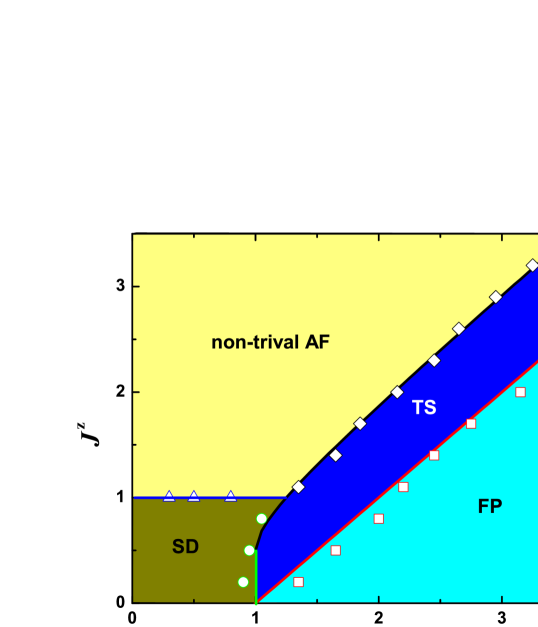
Figure 1: (Color online) The phase diagram with $J^{x}=0$. The solid lines and scattering lines come from bond operator theory and quantum Monte Carlo, respectively. The phase diagram contains an antiferromagnet (AF), a singlet dimer (SD), a triplon solid (TS) and fully polarized state (FP).

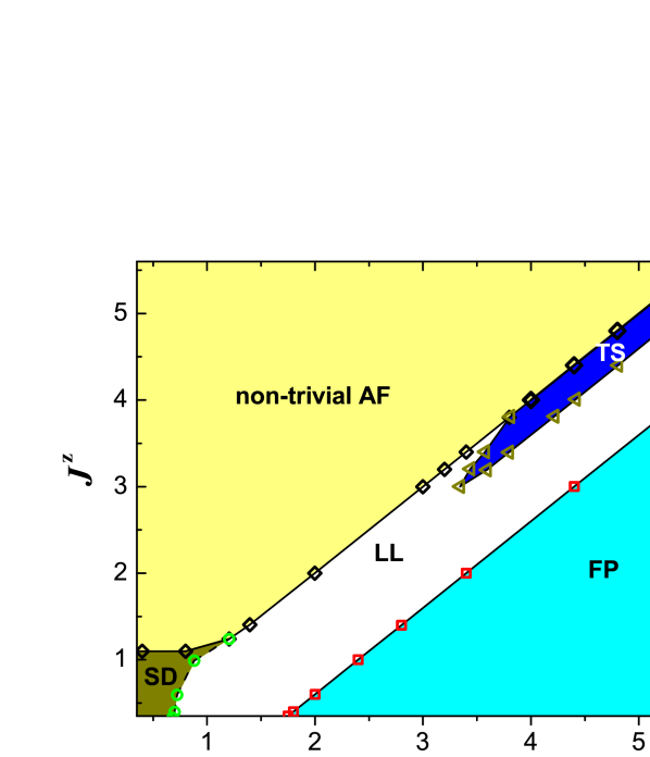
Figure 2: (Color online) Ground state phase diagram with $J^{x}=0.35$. The scatter lines (Black) are QMC results. There are four orders which are antiferromagnetic (AF), full polarized (FP), and Luttinger liquid (LL).

3.1 Full polarized and singlet dimer phases

First, let us see two simplest limits. The first is the full polarized (FP) state in large enough field $h$. The second occurs at $J^{x}=J^{z}=0$, where the Hamiltonian (1) reduces to an array of disjoint dimers. In the second limit, the ground state and excitations are determined by individual dimers. The energies of singlet and triplets are $E(s_{j})=-3K/4$, $E(t_{+,j})=K/4-h$, $E(t_{0,j})=K/4$, $E(t_{-,j})=K/4+h$. When $h=0$, the ground state is an array of singlets (we call it singlet dimer (SD) phase) with an excitation gap $\Delta_{1}=K$. With the applied field $h$ increasing, the system’s ground state experiences a transition from SD to FP state at $h=\Delta_{1}$.

3.2 Triplon solid

If we fix $J^{x}=0$ and raise $J^{z}>0$ ($<1$), a triplon solid (TS) phase intervenes between SD and FP phases (Figure 1). The TS state is a paving of singlets and triplets on the ladders alternatively. To detect the TS order in a general case, one can define a triplon creation operator $d_{i}^{{\dagger}}$ acting in spin’s Hilbert space

$$d_{j}^{{\dagger}}=\frac{1}{\sqrt{2}}(S_{1,j}^{+}-S_{2,j}^{+}).$$ (3)

We have $d_{j}^{{\dagger}}|t_{-}\rangle_{j}=|s\rangle_{j}$, $d_{j}^{{\dagger}}|s\rangle_{j}=|t_{+}\rangle_{j}$, and $d_{j}^{{\dagger}}|t_{+}\rangle_{j}=0$ . It is worth noting that $d_{j}^{{\dagger}}$ is not a perfect hardcore boson [16]. But with appropriate model parameters, the hardcore condition could be well fulfilled. The diagonal real space correlation function of triplon is defined as

$$C^{zz}(r)=\frac{1}{L}\sum_{j}\langle t_{+,j}^{{\dagger}}t_{+,j}t_{+,j+r}^{{\dagger}}t_{+,j+r}\rangle,$$ (4)

where the thermodynamic limit $L\rightarrow\infty$ is taken. The static structure factor for detecting TS order is given by

$$S(Q)=\frac{1}{L}\sum_{r}C^{zz}(r)e^{\mathbf{i}Qr}.$$ (5)

From the point of view of renormalization, the $|t_{0}\rangle_{j}$ and $|t_{-}\rangle_{j}$ states could be projected out from Hilbert space in a moderate strong external field, which breaks the time-reversal symmetry (TRS). Thus we get a reduced constraint $s_{j}^{{\dagger}}s_{j}+t_{+,j}^{{\dagger}}t_{+,j}=1$, so that the Hamiltonian (2) at low energy sector can be replaced by

$$H_{1}=\frac{J^{z}}{2}\sum_{j}\tau_{j}^{z}\tau_{j+1}^{z}-\left(h-K-\frac{J^{z}}{2}\right)\sum_{j}\tau_{j}^{z}+L\left(\frac{J^{z}}{8}-\frac{K}{4}-\frac{h}{2}\right),$$ (6)

where we have defined the pseudo-spin operators in a Schwinger boson representation, $\tau_{j}^{{\dagger}}=t_{+,j}^{{\dagger}}s_{j},\tau_{j}^{-}=t_{+,j}s_{j}^{{\dagger}},\tau_{j}^{z}=(t_{+,j}^{{\dagger}}t_{+,j}-s_{j}^{{\dagger}}s_{j})/2$. The effective Hamiltonian (6) is nothing but a ”classical Ising model in a field”. The TS phase is a consequence of the first antiferromagnetic interaction term. If the second term prevails the first one, SD and FP phases could be reached if $\left(h-K-\frac{J^{z}}{2}\right)<0$ and $\left(h-K-\frac{J^{z}}{2}\right)>0$ respectively. We also get the phase boundaries by comparing the ground state energies of the three states: (i) $h=K$ for the boundary between SD and TS and (ii) $J^{z}=h-K$ between TS and FP. It is worth to point out that the effective Hamiltonian (6) also gives a good description for TS and FP phase in the phase diagram where $J^{z}>1$. The consistency between the analytical and numerical results are quite well, as shown in Figure 3.

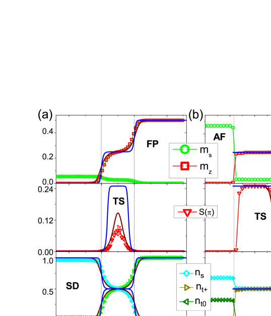
Figure 3: (Color online) The order parameters defined by Eq.(5) and (18) and the densities of state $|s\rangle,|t_{+}\rangle,|t_{0}\rangle$ per rung. The selected parameters are $J^{x}=0,J^{z}=0.5$ in (a) and $J^{x}=0,J^{z}=1.5$ in (b). The scattered lines represent QMC results with $L=100$. The wine-colored solid lines are results obtained from bond operator theory with $L=100$ (blue lines are for $L=300$).

3.3 Luttinger liquid

If $J^{x}\neq 0$, the area of TS phase shrinks to the top right corner of the phase diagram (Figure 2) and there emerges a vast gapless phase called Luttinger liquid (LL). In isotropic case, i.e., $J^{x}=J^{z}$, there have been a large amount of literatures devoted to the study of the ground state and low excitations [17, 18, 19]. Here we focus on the anisotropic case, $J^{z}\neq J^{x}$, and answer the question whether there is still a region described by LL, which, to our knowledge, is not been discussed before. We give a positive answer here.

Interestingly, the low energy properties in the LL phase are also governed by the states $|s\rangle_{j}$ and $|t_{+}\rangle_{j}$. But the effective Hamiltonian includes a part of ”quantum fluctuations” besides the ”classical” part, $H_{1}$,

$$H_{2}=H_{1}+\sum_{j}[\frac{J^{x}}{2}(\tau_{j}^{+}\tau_{j+1}^{-}+h.c)].$$ (7)

This model is exactly the form of the $XXZ$ chain whose properties are well known owing to many reliable methods, such as Bethe Ansatz and bosonization. We know that its ground state is antiferromagnet or LL when $J^{z}/J^{x}>2$ or $J^{z}/J^{x}<2$ respectively [20]. In LL, both diagonal and off-diagonal triplon correlations are important. The former is defined in (5). The latter can be defined as

$$C^{+-}(r)=\frac{1}{L}\sum_{j}\langle d_{j}^{{\dagger}}d_{j+r}\rangle.$$ (8)

From the effective model (7), we can get the equal-time spin correlation by the standard Abelian bosonization techniques [21],

$$C^{zz}(r)=\langle\tau_{j+r}^{z}\tau_{j}^{z}\rangle=m_{z}^{2}-\frac{c_{1}}{r^{2}}+\frac{c_{2}}{r^{2K_{L}}}\cos(2\pi m_{z}r),$$ (9)

$$C^{+-}(r)=\langle\tau_{j+r}^{+}\tau_{j}^{-}\rangle=c_{3}\frac{(-1)^{r}}{r^{1/2K_{L}}}-c_{4}\frac{(-1)^{r}}{r^{2K_{L}+1/2K_{L}}}\cos(2\pi m_{z}r),$$ (10)

where $r$ denotes the lattice distance, $c_{1},c_{2},c_{3},c_{4}$ are constants, $m_{z}=(1/2N)\sum_{j}\langle(S_{1,j}^{z}+S_{2,j}^{z})\rangle$ is the uniform magnetization, $K_{L}$ is the so-called LL parameter with typical value less than $0.5$ that governs the spin correlations at long wavelength limit. For a comparison, we perform the QMC simulation on the original Hamiltonian (1). We found the spin ladder is sensitive to the value of $J^{x}$ in TS region. However, comparing with spin $XXZ$ chain, the TS and LL still exist in the phase diagram of the spin ladder only with quantitative changes of phase boundaries. The densities of four rung states $|s\rangle,|n_{t+}\rangle,|n_{t0}\rangle,|n_{t-}\rangle$ shown in Figure 4(b) confirm the goodness of the effective model (7). From the nodes of structure factor $S(\pi)$ in Figure 4(a), we can see a clear phase transition from TS to LL. The long range diagonal order in TS also could be seen in the correlation function $C^{zz}(r)$ of Figure 4(d). In Figure 4(c) we show the power law decay behavior of correlation $C^{+-}(r)$ in LL region, which coincides with the relation (10) perfectly.

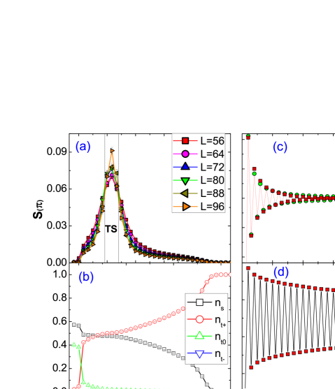
Figure 4: (Color online) (a) The structure factor $S(\pi)$ in $h=3.8$ obtained by QMC in different lattice sizes. (b) The densities of four states in each rung. (c) The correlation function $C^{+-}(r)$ where the square scattered line is obtained from QMC and the circular scattered line comes from fitting Eq.(10). (d) The correlation function $C^{zz}(r)$ with long range order in $h=3.3$. Here, the selected parameters are $J^{x}=0.35,J^{z}=3.0$.

3.4 Non-trivial antiferromagnetic phase

Now we turn to the last phase. First, we focus on the thermodynamic limit, and the case of $J^{x}=0$ (see Figure 1), since the qualitative properties do not change if $J^{x}$ is not large enough. We show the ground state phase is a gapped Mott insulator of triplon that can be understood quite good by an effective Ising model in a transverse field (T-Ising model). Then we will work on finite system to figure out the low excitations of this phase. We will show the lowest two states for finite systems are nearly degenerate and tend to be maximally entangled with $J^{z}$ increasing.

3.4.1 Two channels

When $h$ is small and $J^{z}$ is large enough, the low energy sector of the system splits into two channels. The first one (channel A) is a classical Ising Hamiltonian

$$H_{A}=2J^{z}\sum_{j}\eta_{j}^{z}\eta_{j+1}^{z}-2h\sum_{j}\eta_{j}^{z}+\frac{LK}{4},$$ (11)

with $\eta_{j}^{z}=\frac{1}{2}(t_{+,j}^{{\dagger}}t_{+,j}-t_{-,j}^{{\dagger}}t_{-,j})$ and constraint $t_{+,j}^{{\dagger}}t_{+,j}+t_{-,j}^{{\dagger}}t_{-,j}=1$. When $h=0$, the gound state is an alternative paving of $|t_{+}\rangle_{j}$ and $|t_{-}\rangle_{j}$ states along the ladders. Its lowest energy per rung reads

$$E_{0,A}/L=\frac{K}{4}-\frac{J^{z}}{2}.$$ (12)

The second one (channel B) is obtained by introducing a set of pseudo-spin operators in another Schwinger boson representation, $\lambda_{j}^{+}=s_{j}^{{\dagger}}t_{0,j}$, $\lambda_{j}^{-}=s_{j}t_{0,j}^{{\dagger}}$, $\lambda_{j}^{z}=(s_{j}^{{\dagger}}s_{j}-t_{0,j}^{{\dagger}}t_{0,j})/2$, with constraint $s_{j}^{{\dagger}}s_{j}+t_{0,j}^{{\dagger}}t_{0,j}=1$, which reads

$$H_{B}=\sum_{j}[2J^{z}\lambda_{j}^{x}\lambda_{j+1}^{x}-K\lambda_{j}^{z}-K/4].$$ (13)

This is exactly the T-Ising model, whose properties are also well-known. One can solve it exactly by applying the Jordan-Wigner transformation [22], and get the lowest energy per rung,

$$E_{0,B}/L=-\frac{K}{4}-\frac{J^{z}(J^{z}+K)}{\pi}E\left(\frac{4J^{z}K}{(J^{z}+K)^{2}}\right),$$ (14)

where $E(x)$ is the complete elliptic integral of the second kind. Because the field $h$ is coupled with $t_{i,+}$ and $t_{i,-}$, it does not appear in channel B. In fact, this is the reason why the phase boundary between SD and AF phases is a straight line (see Figure 1 and 2) that almost does not change with the field increasing for a given $J^{x}$ until runs into another phase. In the following, combining numerical approaches, we emphasize several important consequences of the above effective Hamiltonians. It is easy to see that the difference of the lowest energies between channels A and B is

$$\Delta=E_{0,A}/L-E_{0,B}/L>K/2.$$ (15)

So we see that channel B truly reflects the ground state of the original ladders system. In the whole parameter region, channel B gives quite good description of the ground state energy of original system. The goodness of effective $H_{B}$ for the ground state has been confirmed by QMC simulations on the original ladders system shown in Figure 3, 4, and 5.

3.4.2 Quantum phase transition in thermodynamic limit

In thermodynamic limit and when $J^{z}>K$, the effective Hamiltonian $H_{B}$ exhibits an AF phase with double degeneracy,

$$|\psi_{1}^{AF}\rangle = \prod_{j}\otimes\left(|s\rangle_{j}+(-1)^{j}|t_{0}\rangle_{j}\right),$$ (16)

$$|\psi_{2}^{AF}\rangle = \prod_{j}\otimes\left(|s\rangle_{j}-(-1)^{j}|t_{0}\rangle_{j}\right).$$ (17)

This result needs an assumption of spontaneous symmetry breaking nevertheless. We will address this issue later. The staggered magnetization of this phase can be detected by the order parameter

$$m_{s}=\frac{1}{2L}\sum_{i}(-1)^{i}\langle(S_{1,j}^{z}-S_{2,j}^{z})\rangle.$$ (18)

There is a quantum phase transition between the SD and AF phases at the gapless point $J^{z}=K$, which can be worked out from the divergence point of the second-order derivative of $E_{0,B}$ on $J^{z}$, as well as the first-order derivative of the weight of singlets

$$n_{s}\equiv\frac{1}{L}\sum_{j}\langle s_{j}^{{\dagger}}s_{j}\rangle=\frac{1}{2\pi}\int_{-\pi}^{\pi}dk\frac{(J^{z}\sin k)^{2}}{2\omega(k)\left(\omega(k)+J^{z}\cos k-K\right)},$$ (19)

where

$$\omega(k)=\sqrt{(J^{z}\cos k-K)^{2}+(J^{z}\sin k)^{2}}$$ (20)

is the lowest excitation spectrum of $H_{B}$. The staggered magnetization $m_{s}$ is deduced from the correlation function $\langle\lambda_{i}^{x}\lambda_{j}^{x}\rangle$ formally, which is too tedious to be presented here. The smooth curve in Figure 5(a) shows $m_{s}$ that is obtained by the correlation function with $\max|i-j|=160$. Comparing it with QMC results, we confirm the validity of the effective Hamiltonian $H_{B}$. The phase transition between those two states is of second order, which can be seen from the staggered magnetic susceptibility $\chi_{s}$ shown in Figure 5(b).

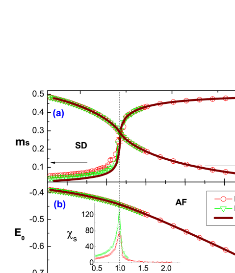
Figure 5: (Color online) (a) The staggered magnetization and the density of singlet state per rung. (b) The energy per site and the inserted one is staggered magnetic susceptibility. Here the scattered lines are obtained from QMC, the solid line are analytic results of effective Hamiltonian (13). The QMC is simulated in a ladder with $J^{x}=0$, $h=0.5$.

3.4.3 Exact diagonalization of finite systems

Is the effective Hamiltonian $H_{B}$ good enough for low excitations? How do the translational and TRS breaking happen in the AF phase for the original ladders system? To answer these questions, we performed an exact diagonalization on the original system up to $L=10$ (i.e. $20$ sites) to reveal the aspect of the original system that may be ignored. We found, although the effective $H_{B}$ reflects the ground state of the original system perfectly, the low excitations above the ground state is largely restricted by channel A. The excitation spectrum (20) of channel B gives an energy gap above its ground state,

$$\Delta_{gap}^{B}=\left|J^{z}-K\right|.$$ (21)

But the true gap of the original system should not exceed $\Delta$ (see (15)), so in large $J_{z}$ we have

$$\Delta_{gap}=\min(\Delta,\Delta_{gap}^{B}).$$ (22)

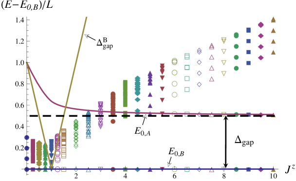
Figure 6: (Color online) Discrete energy levels for a ladder with length $L=10$ (labelled by colored markers) obtained by exact diagonalization and analytical results for a ladder with $L\rightarrow\infty$ (shown by lines) obtained by effective theories. The dashed line represents the true gap at large $J_{z}$ limit. Here $J^{x}=0$ and $K=1$ are taken. Please see more details in the text.

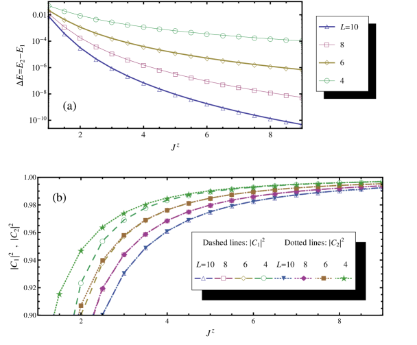
Figure 7: (Color online) (a) The energy difference, $\Delta E=E_{2}-E_{1}$, of the lowest two states, $\left|\phi_{1}\right\rangle$ and $\left|\phi_{2}\right\rangle$. (b) The percentages, $|C_{1}|^{2}$ and $|C_{2}|^{2}$, of dominant parts in the lowest two states. Please see more in the text.

The numerical result for $J^{x}=0$ is exemplified in Figure 6. We see the excitations of the ladder system is much different from the effective $H_{B}$. In large $J^{z}$, we observe no extra energy levels lying between $E_{0,A}$ and $E_{0,B}$, which ensures a true gap greater than $K/2$. Another observation is the lowest two levels of finite systems are not exactly degenerate and not even the ones with AF order, $|\psi_{1}^{AF}\rangle$ and $|\psi_{2}^{AF}\rangle$. Instead, they are

$$\left|\phi_{1}\right\rangle = \frac{C_{1}}{\sqrt{2}}\left(|\psi_{1}^{AF}\rangle+|\psi_{2}^{AF}\rangle\right)+res.,$$ (23)

$$\left|\phi_{2}\right\rangle = \frac{C_{2}}{\sqrt{2}}\left(|\psi_{1}^{AF}\rangle-|\psi_{2}^{AF}\rangle\right)+res.,$$ (24)

with dominant parts prevail the residuals. The numerical results are shown in Figure 7. We observed that $\left|\phi_{1}\right\rangle$ has slightly lower energy than $\left|\phi_{2}\right\rangle$, but their energy difference $\Delta E=E_{2}-E_{1}$ rapidly reduces to zero with $J_{z}$ increasing. And, at the same time, the two states approach the so-called GHZ states [23] asymptotically,

$$\left|\phi_{1}\right\rangle \approx \frac{1}{\sqrt{2}}\left(|\psi_{1}^{AF}\rangle+|\psi_{2}^{AF}\rangle\right),$$ (25)

$$\left|\phi_{2}\right\rangle \approx \frac{1}{\sqrt{2}}\left(|\psi_{1}^{AF}\rangle-|\psi_{2}^{AF}\rangle\right).$$ (26)

The result implies the entangled GHZ states could be purified if we increase $J^{z}$ adiabatically for finite system. For long enough system, spontaneous symmetry breaking may occur and the entanglement will vanish. Nonetheless, the two GHZ states do not exhibit a non-zero order parameter $m_{s}$, while they do have the same antiferromagnetic spin correlation functions as $|\psi_{1}^{AF}\rangle$ and $|\psi_{2}^{AF}\rangle$. That is the reason why we name it a non-trivial AF phase. One can check that $\left|\phi_{1}\right\rangle$ and $\left|\phi_{2}\right\rangle$ are eigenstates of the time reversal operator

$$\Theta=\prod\limits_{j,l}\otimes\left(-\mathbf{i}\sigma_{l,j}^{y}\right)\kappa,$$ (27)

where $\kappa$ is the complex conjugation, if noticing that

$$\Theta s_{j}^{{\dagger}}\Theta^{{\dagger}} = s_{j}^{{\dagger}},$$ (28)

$$\Theta t_{0,j}^{{\dagger}}\Theta^{{\dagger}} = -t_{0,j}^{{\dagger}}.$$ (29)

Thus $\left|\phi_{1}\right\rangle$ and $\left|\phi_{2}\right\rangle$ preserve the exact TRS as the same as the original Hamiltonian (1). From the point of view of the effective $H_{B}$, the assumption of spontaneous symmetry breaking in thermodynamic limit is based an unpredictable disturbance from environment [22]. But here we have one favorable factor to avoid this - the destructive field should couple to local variables, $\lambda_{j}^{x}=(s_{j}^{{\dagger}}t_{0,j}+s_{j}t_{0,j}^{{\dagger}})/2$, delicately since the system with true gap is antiferromangetic. Thus we think there is the chance to realize such entangled states that do not break the TRS.

4 Discussion

The dimer $XXZ$ spin system discussed in this paper might be realized in a Mott insulating phase of cold bosonic atoms in near future [8, 9]. We can estimate the typical energy scales. For ⁸⁷Rb atoms with a lattice constant $\pi/k_{x}\simeq 2\pi/k_{y}\sim 426$ nm and about $10^{5}$ atoms in a Bose-Einstein condensate, we can chose $t^{2}/(\hbar U)\sim 0.1$ kHz (corresponding to a time scale of 10 ms) with a conservative choice of $U\sim$ $2$ kHz and $(t/U)^{2}\sim 1/20$, where $t$ is the hopping strength of cold atoms between two nearest neighbor minimums of laser potential and $U$ is on site interaction originating from the $s$ wave scattering. These energy scales are clearly compatible with current experiments [4] and make the system in a Mott insulating area. In experiment, the density of condensates in momentum space $\langle\tilde{n}_{\pi}\rangle$ can be measured by noise correlations which can be linked to spin-spin correlations [24, 25, 26]. We can use Bragg scattering of light, which gives rise to the spin structure factor, to detect $S(\pi)$ [27]. An alternative technique for imaging spin states in optical lattices has been put forward [28]. Thus, all the phases discussed in this paper are detectable in experiment.

5 Summary

In summary, combining analytical and numerical methods, we have investigated the ground state phase diagrams and low excitations of the dimer $XXZ$ spin ladder system. We show that most features of the phases could be understood within the frame of bond operator theory and have proven it by using quantum Monte Carlo method. We present the rich ground state phase diagram which can be detected in optical lattice by future experiment.

6 Acknowledgments

This work was supported by the NSFC under grants No. 11074177, SRF for ROCS SEM (20111139-10-2)

References

References

- [1] Dagotto E and Rice T M 1996 Science 271 5249
- [2] Bouillot P et al 2011 Phys. Rev. B 83 054407, and references therein.
- [3] Jaksch D, Bruder C, Cirac J I, Gardiner C W and Zoller P 1998 Phys. Rev. Lett. 81 3108
- [4] Greiner M et al 2002 Nature (London) 415 39
- [5] Duan L M, Demler E and Lukin M D 2003 Phys. Rev. Lett. 91 090402
- [6] Sebby-Strabley J, Anderlini M, Jessen P S and Porto J V 2006 Phys. Rev. A 73 033605
- [7] Fölling S et al 2007 Nature (London) 448 1029
- [8] Trotzky S et al 2008 Science 319 295
- [9] Chen Y A, Nascimbéne S, Aidelsburger M, Atala M, Trotzky S and Bloch I 2011 Phys. Rev. Lett. 107 210405
- [10] Crépin F, Laflorencie N, Roux G and Simon P 2011 Phys. Rev. B 84 054517
- [11] Masubara T and Matsuda H 1956 Prog. Theor. Phys. 16 569
- [12] Paredes B, Widera A, Murg V, Mandel O, Fölling S, Cirac I, Shlyapnikov G V, Hänsch T W and Bloch I 2004 Nature (London) 429 277
- [13] He P B, Sun Q, Li P, Shen S Q and Liu W M 2007 Phys. Rev. A 76 043618
- [14] Sandvik A W 1999 Phys. Rev. B 59 R14157
- [15] Syljuasen O F and Sandvik A W 2002 Phys. Rev. E 66 046701
- [16] Ng K K and Lee T K 2006 Phys. Rev. B 73 014433
- [17] Furusaki A and Zhang S C 1999 Phys. Rev. B 60 1175
- [18] Laflorencie N and Mila F 2007 Phys. Rev. Lett. 99 027202
- [19] Giamarchi T and Tsvelik A M 1999 Phys. Rev. B 59 11398
- [20] Yang C N and Yang C P 1966 PR 150 321
- [21] Hikihara T and Furusaki A 2001 Phys. Rev. B 63 134438
- [22] Kitaev A and Laumann C arXiv:0904.2771
- [23] Greenberger D M, Horne M and Zeilinger A 1990 Am. J. Phys. 58 1131
- [24] Altman E, Demler E and Lukin M D 2004 Phys. Rev. A 70 013603
- [25] Fölling S et al 2005 Nature (London) 434 481
- [26] Scarola V W et al 2006 Phys. Rev. A 73 051601(R)
- [27] Corcovilos T A et al 2010 Phys. Rev. A 81 013415
- [28] Douglas J and Burnett K 2010 Phys. Rev. A 82 033434