Methods for Analyzing Resonances in Atomic Scattering
Taha Sochi  and P.J. Storey
University College London, Department of Physics and Astronomy, Gower Street, London, WC1E 6BT

Abstract

Resonances, which are also described as autoionizing or quasi-bound states, play an important role in the scattering of atoms and ions with electrons. The current article is an overview of the main methods, including a recently-proposed one, that are used to find and analyze resonances.

Keywords: atomic scattering; resonance; autoionizing states; quasi-bound states; R-matrix; K-matrix method; QB method; time-delay method.

1 Introduction

In atomic scattering, resonance occurs when a colliding continuum electron is captured by an ion to form a doubly excited state. The resonant state is normally short lived and hence it is permanently stabilized either by a radiative decay of the captured electron or an electron in the parent to a true bound state of the excited core ion or by autoionization to the continuum with the ejection of an electron. In most cases the stabilization occurs through the second route, i.e. by autoionization rather than radiative decay. These excited autoionizing systems leave a distinctive signature in the cross sections for electron scattering processes. The Auger effect is one of the early examples of the resonance effects that have been discovered and extensively investigated [1, 2, 3]. The reader is advised to consult other references in the literature of atomic physics (e.g. [1, 4]) for a general historical background.

Symmetric and asymmetric line shapes have been proposed to model resonance profiles for different situations; these profiles include Lorentz, Shore and Fano, as given in Table 1. Resonance characteristics; such as their position on the energy axis, area under profile and full width at half maximum; are usually obtained by fitting the profile of the autoionizing state to a fitting model such as Lorentz. These characteristics have physical significance; for example the width of a resonance quantifies the strength of the interaction with the continuum and hence autoionization probability and lifetime, while the contribution of a resonance to a photoionization cross section, quantified by the area beneath it, is related to the probability of radiative decay [5, 4, 6, 7, 8].

Table 1: The commonly-used resonance line profiles where $\sigma$ is the photoionization cross section, $A$ is a proportionality factor with the dimension of area, $\Delta_{E}$ is the full width at half maximum, $E$ is the energy, $E_{r}$ is the resonance position on the energy line, $p=\frac{2\left(E-E_{r}\right)}{\Delta_{E}}$, $\alpha$ and $\beta$ are parameters related to the dipole and Coulomb matrix elements, and $k$ is the Fano asymmetry factor.

Profile	Equation
Lorentz	$\sigma=A\frac{\Delta_{E}^{2}/4}{\left(E-E_{r}\right)^{2}+\Delta_{E}^{2}/4}$
Shore	$\sigma=A\frac{\alpha p+\beta}{p^{2}+1}$
Fano	$\sigma=A\frac{\left(k+p\right)^{2}}{p^{2}+1}$

2 Methods for Investigating Resonances

There are several methods for finding and analyzing resonances. In the following sections we outline three of these methods which are all based on the use of the reactance K-matrix of the R-matrix theory for atomic and molecular scattering calculations. The advantage of this common approach, which employs the close coupling approximation, is that resonance effects are naturally delineated, since the interaction between bound and free states is incorporated in the scattering treatment.

2.1 QB Method

A common approach for finding and analyzing resonances is to apply a fitting procedure to the reactance matrix, K, or its eigenphase as a function of energy in the neighborhood of an autoionizing state. However, fitting the K-matrix itself is complicated because the reactance matrix has a pole at the energy position of the autoionizing state. An easier alternative is to fit the arc-tangent of the reactance matrix. The latter approach was employed by Bartschat and Burke [2] in their fitting code RESFIT.

The eigenphase sum is defined by

$$\delta=\sum_{i=1}^{N}\arctan\Lambda_{i}$$ (1)

where $\Lambda_{i}$ is an eigenvalue of the K-matrix and the sum runs over all open channels interacting with the autoionizing state. The eigenphase sum is normally fitted to a Breit-Wigner form

$$\delta=\overline{\delta}+\arctan\left(\frac{\Delta_{r}}{2\left(E_{r}-E\right)}\right)$$ (2)

where $\overline{\delta}$ is the sum of the background eigenphase and $\Delta_{r}$ is the resonance width. This approach was used by Tennyson and Noble [9] in their fitting code RESON [10].

In theory, an autoionizing state exhibits itself as a sharp increase by $\pi$ radians in the eigenphase sum as a function of energy superimposed on a slowly-varying background. However, due to the finite width of resonances and the background variation over their profile, the increase may not be by $\pi$ precisely in the actual calculations. A more practical approach then is to identify the position of the resonance from the energy location where the increase in the eigenphase sum is at its highest rate by having a maximum gradient with respect to the scattering energy, i.e. $\left(d\delta/dE\right)_{max}$ [9, 11, 12].

The QB method of Quigley and Berrington [11] is a computational technique for finding and analyzing autoionizing states that arise in atomic and molecular scattering processes using eigenphase fitting. The essence of this method is to apply a fitting procedure to the reactance matrix eigenphase near the resonance position using the analytic properties of the R-matrix theory. The merit of the QB method over other eigenphase fitting procedures is that it utilizes the analytical properties of the R-matrix method to determine the variation of the reactance matrix with respect to the scattering energy analytically. This analytical approach can avoid possible weaknesses, linked to the calculations of K-matrix poles and arc-tangents, when numerical procedures are employed instead. The derivative of the reactance matrix with respect to the scattering energy in the neighborhood of a resonance can then be used in the fitting procedure to identify the energy position and width of the resonance.

The QB method begins by defining two matrices, Q and B, in terms of asymptotic solutions, the R-matrix and energy derivatives, such that

$$\frac{d{\bf{K}}}{dE}={\bf{B}}^{-1}{\bf{Q}}$$ (3)

The gradients of the eigenphases of the K-matrix with respect to energy can then be calculated. This is followed by identifying the resonance position, $E_{r}$, from the point of maximum gradient at the energy mesh, and the resonance width, $\Delta_{r}$, which is linked to the eigenphase gradient at the resonance position, $\delta^{{}^{\prime}}(E_{r})$, by the relation

$$\Delta_{r}=\frac{2}{\delta^{{}^{\prime}}(E_{r})}$$ (4)

This equation may be used to calculate the widths of a number of resonances in a first approximation. A background correction due to overlapping profiles can then be introduced on these widths individually to obtain a better estimate.

The QB method was implemented in the STGQB code of Quigley and coworkers [13] as an extension to the R-matrix code. It should be remarked that Busby et al [12] have used a similar method for finding and analyzing resonances graphically by their VisRes program.

2.2 Time-Delay Method

The Time-Delay method of Stibbe and Tennyson [14] is based on the time-delay theory of Smith [15] where use is made of the lifetime eigenvalues to locate the resonance position and identify its width. According to this theory, the time-delay matrix M is defined in terms of the scattering matrix S by

$${\bf{M}}=-\textrm{i}\,\hbar\,{\bf{S}}^{*}\frac{d{\bf{S}}}{dE}$$ (5)

where i is the imaginary unit, $\hbar$ ($=h/2\pi$) is the reduced Planck’s constant, and ${\bf{S}}^{*}$ is the complex conjugate of ${\bf{S}}$. It has been demonstrated by Smith [15] that the eigenvalues of M represent the collision lifetimes and the largest of these eigenvalues corresponds to the longest time-delay of the scattered particle. For a resonance, the time-delay has a Lorentzian profile with a maximum precisely at the resonance position. By computing the energy-dependent time-delay from the reactance matrix, and fitting it to a Lorentzian peak shape, the resonance position can be located and its width is identified.

This method, as implemented in the TIMEDEL program of Stibbe and Tennyson [14], uses the reactance K-matrix as an input, either from a readily-available archived scattering calculations or from dynamically-performed computations on an adjustable mesh. The S-matrix is then formed using the relation

$${\bf{S}}=\frac{{\bf{I}}+\textrm{i}{\bf{K}}}{{\bf{I}}-\textrm{i}{\bf{K}}}$$ (6)

where ${\bf{I}}$ is the identity matrix. The time-delay M-matrix is then calculated from Equation 5, with numerical evaluation of the S-matrix derivative, and diagonalized to find the eigenvalues and hence obtain the longest time-delay of the incident particle. Approximate resonance positions are then identified from the energy locations of the maxima in the time-delay profile, and the widths are estimated from the Lorentzian fit. On testing the degree of overlapping of neighboring resonances, TIMEDEL decides if the resonances should be fitted jointly or separately.

2.3 K-Matrix Method

Sochi [8] and Sochi & Storey [7] studied the properties of autoionizing states of the C²⁺+e^- system at energies close to the ionization limit. In this, and other Be-like systems, there is only one open channel per angular momentum symmetry and the K-matrix is a real scalar. This simplification makes it possible to directly analyze the poles in K to derive resonance properties as outlined below.

According to the collision theory of Smith [15], M-matrix is related to S-matrix by Equation 5. Now, a single-channel K-matrix with a pole at energy $E_{0}$ superimposed on a background $K_{{}_{o}}$ can be approximated by

$$K_{i}=K_{{}_{o}}+\frac{\rm{g}}{E_{i}-E_{0}}$$ (7)

where $K_{i}$ is the value of the K-matrix at energy $E_{i}$ and $\rm{g}$ is a physical parameter with dimension of energy. In Appendix A it is demonstrated that in the case of single-channel scattering the M-matrix is real with a value given by

$$M=\frac{-2\rm{g}}{(1+K_{{}_{o}}^{2})(E-E_{0})^{2}+2K_{{}_{o}}\rm{g}(E-E_{0})+\rm{g}^{2}}$$ (8)

Using the fact demonstrated by Smith [15] that the lifetime of the state is the expectation value of $M$, it can be shown from Equation 8 that the position of the resonance peak $E_{r}$ is given by

$$E_{r}=E_{0}-\frac{K_{{}_{o}}\rm{g}}{1+K_{{}_{o}}^{2}}$$ (9)

while the full width at half maximum $\Delta_{E}$ is given by

$$\Delta_{E}=\frac{|2\rm{g}|}{1+K_{{}_{o}}^{2}}$$ (10)

Complete derivation of the K-matrix method is given in Appendix A.

The two parameters of primary interest are the resonance energy position $E_{r}$, and the resonance width $\Delta_{r}$ which equals the full width at half maximum $\Delta_{E}$. However, for an energy point $E_{i}$ with a K-matrix value $K_{i}$, Equation 7 has three unknowns, $K_{{}_{o}}$, $\rm{g}$ and $E_{0}$, which are needed to find $E_{r}$ and $\Delta_{r}$. Hence, three energy points in the immediate neighborhood of $E_{0}$ are required to identify these unknowns. As the K-matrix changes sign at the pole, the neighborhood of $E_{0}$ is located by testing the K-matrix value at each point of the energy mesh for a sign change or a discontinuity evidenced by a sharp change in the gradient.

In practical terms, the method of locating the K-matrix poles is as follows. The asymptotic routine STGF [16, 17, 18] in the R-matrix package was modified by the authors to test for a sign change in the value of K as it is calculated, initially using a coarse energy mesh. If a sign change is detected, the new STGF routine goes back in the energy mesh and defines a new fine mesh over very limited energy range that includes the sign-change position and outputs the energy points of the fine mesh and the corresponding K-matrix values to be used for finding the resonance parameters.

The modified STGF also writes the K-matrix values to a file. In case a sign change is not detected, a separate code reads the K-matrix and tests the slope for a sudden change where poles could exist. If such a change is detected a new finer energy mesh around the suspected pole is prepared for a new STGF run. The process is repeated until a sign change is seen in the K-matrix at which point the resonance parameters are computed.

Table 2: The two C ii resonances used for demonstrating the K-matrix poles in Figures 1 and 2. The columns from left to right are: configuration, level, experimental energy in wavenumbers (cm^-1) relative to the ground state, experimental energy in Rydberg relative to the C^{2+ 1}S${}^{\rm{e}}_{{}_{0}}$ limit, theoretical energy in Rydberg from K-matrix calculations relative to the C^{2+ 1}S${}^{\rm{e}}_{{}_{0}}$ limit, full width at half maximum from K-matrix in Rydberg, theoretical energy in Rydberg from QB calculations relative to the C^{2+ 1}S${}^{\rm{e}}_{{}_{0}}$ limit, and full width at half maximum from QB in Rydberg. The experimental data are obtained from the National Institute of Standards and Technology (NIST).

Config.	Lev.	NEEW	NEER	TERK	FWHMK	TERQ	FWHMQ
1s22s2p(3Po)4d	4F${}^{\rm{o}}_{{}_{7/2}}$	219590.76	0.208918	0.209174	5.96E-09	0.209174	5.96E-09
1s22s2p(3Po)4d	4P${}^{\rm{o}}_{{}_{3/2}}$	220832.15	0.220230	0.220680	5.32E-10	0.220680	5.32E-10

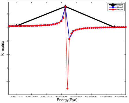
Figure 1: K-matrix as a function of energy for the first resonance in Table 2, using three meshes, a coarse mesh, Mesh1, and two finer meshes, Mesh2 and Mesh3. The K-matrix sign change occurs only with Mesh2 and Mesh3.

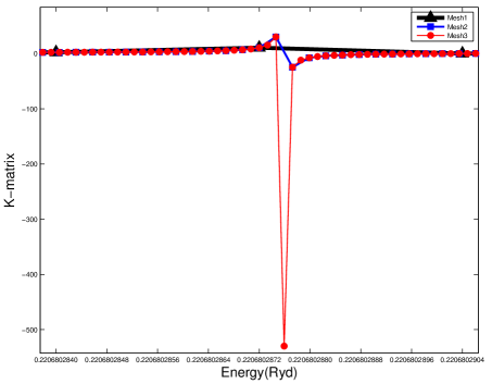
Figure 2: K-matrix as a function of energy for the second resonance in Table 2 using three meshes, a coarse mesh, Mesh1, and two finer meshes, Mesh2 and Mesh3. The K-matrix sign change occurs only with Mesh2 and Mesh3.

The process is demonstrated in Figures 1 and 2 which are based on two examples from the C ii resonances [7] (refer to Table 2 for details). As seen in these figures, the local change in the magnitude of the gradient in the coarse mesh (Mesh1) indicated the possible presence of a pole. The two figures also show that the two finer meshes, Mesh2 with about 10 times more points, and Mesh3 with about 20 times more points, have succeeded in finding the pole through the detection of sign change in the K-matrix although the K-matrix profile is better delineated by Mesh3. For very narrow resonances care must be taken to not compute the K-matrix too close to the pole as numerical noise can cause instability in the derived resonance parameters.

A comparison between the K-matrix and QB on the C ii resonances [8] demonstrated that these methods produce virtually identical results. However, the K-matrix is computationally superior in terms of the required computational resources, mainly CPU time. Moreover, it is more powerful in detecting very narrow resonances which QB cannot find. Nevertheless, the QB method is more general as it deals with multi-channel resonances, as well as single-channel resonances, while the K-matrix method in its current formulation is restricted to single-channel resonances.

3 Conclusions

The resonance phenomenon plays very important role in the atomic scattering processes and subsequent transitions. Several methods based on different theoretical backgrounds have been proposed and used to find resonances and identify their parameters. In this article, we outlined three methods for finding and analyzing resonances, including the recently developed K-matrix method, which is highly efficient for investigating single-channel resonances near the ionization threshold.

4 Appendix A: Using Lifetime Matrix to Investigate Single-Channel Resonances

In this Appendix we present the K-matrix method which is based on using the lifetime matrix ${\bf{M}}$ expressed in terms of the reactance matrix ${\bf{K}}$ to investigate single-channel resonances.

In the case of single-channel states, M, S and K are one-element matrices. To indicate this fact we annotate them with $M$, $S$ and $K$. From Equations 5 and 6, the following relation can be derived

$$M=\frac{2}{1+K^{2}}\frac{dK}{dE}$$ (11)

It is noteworthy that since $K$ is real, $M$ is real as it should be.

Smith [15] has demonstrated that the expectation value of $M$ is the lifetime of the state, $\tau$. Now if we consider a K-matrix with a pole superimposed on a background $K_{{}_{o}}$

$$K=K_{{}_{o}}+\frac{\rm{g}}{E-E_{0}}$$ (12)

then from Equation 11 we find

$$M(E) = \frac{-2\rm{g}}{(1+K^{2})(E-E_{0})^{2}}$$ (13)

$$= \frac{-2\rm{g}}{(1+K_{{}_{o}}^{2})(E-E_{0})^{2}+2K_{{}_{o}}\rm{g}(E-E_{0})+\rm{g}^{2}}$$

The maximum value of $M(E)$ occurs when the denominator has a minimum, that is when

$$E=E_{0}-\frac{K_{{}_{o}}\rm{g}}{1+K_{{}_{o}}^{2}}$$ (14)

and hence

$$M_{max}=-\frac{2(1+K_{{}_{o}}^{2})}{\rm{g}}$$ (15)

This reveals that by including a non-vanishing background the peak of $M$ is shifted relative to the pole position, $E=E_{0}$, and the peak value is modified. If we now calculate the full width at half maximum, $\Delta_{E}$, by locating the energies where $M=\frac{1}{2}M_{max}$ from solving the quadratic

$$(1+K_{{}_{o}}^{2})(E-E_{0})^{2}+2K_{{}_{o}}\rm{g}(E-E_{0})-\frac{\rm{g}^{2}(1-K_{{}_{o}}^{2})}{(1+K_{{}_{o}}^{2})}=0$$ (16)

we find

$$\Delta_{E}=\frac{|2\rm{g}|}{1+K_{{}_{o}}^{2}}$$ (17)

The two main parameters in the investigation of autoionizing states are the resonance energy position $E_{r}$ and its width $\Delta_{r}$. For an energy point $E_{i}$ with a K-matrix value $K_{i}$, Equation 12 contains three unknowns, $K_{{}_{o}}$, $\rm{g}$ and $E_{0}$ which are required to obtain $E_{r}$ and $\Delta_{r}$, and hence three energy points at the close proximity of $E_{0}$ are required to identify the unknowns. Since the K-matrix changes sign at the pole, the neighborhood of $E_{0}$ is detected by inspecting the K-matrix at each point on the energy mesh for sign reversal and hence the three points are obtained accordingly. Now, if we take the three consecutive values of $K$

$$K_{i}=K_{{}_{o}}+\frac{\rm{g}}{E_{i}-E_{0}}\verb| |(i=1,2,3)$$ (18)

and define

$$\Delta E_{jk}=E_{j}-E_{k}\verb| |\&\verb| |\Delta K_{jk}=K_{j}-K_{k},$$ (19)

then with some algebraic manipulation we find for $E_{0}$, $\rm{g}$ and $K_{{}_{o}}$,

$$\boxed{E_{0}=\frac{E_{1}\Delta K_{12}\Delta E_{32}-E_{3}\Delta K_{23}\Delta E_{21}}{\Delta K_{12}\Delta E_{32}-\Delta K_{23}\Delta E_{21}}}$$ (20)

$$\boxed{\rm{g}=\frac{\Delta K_{12}\Delta E_{10}\Delta E_{20}}{\Delta E_{21}}}$$ (21)

and

$$\boxed{K_{{}_{o}}=K_{1}-\frac{\rm{g}}{\Delta E_{10}}}$$ (22)

Finally, $E_{r}$ and $\Delta_{r}$ can be computed from Equation 14 and Equation 17 respectively. Full details are given in [8].

References

- [1] Burke P.G. Resonances in electron scattering and photon absorption. Advances in Physics, 14(56):521–567, 1965.
- [2] Bartschat K.; Burke P.G. Resfit - A multichannel resonance fitting program. Computer Physics Communications, 41(1):75–84, 1986.
- [3] Storey P.J.; Sochi T. Electron temperatures and free-electron energy distributions of nebulae from C ii dielectronic recombination lines. Monthly Notices of the Royal Astronomical Society, 430(1):599–610, 2013.
- [4] Drake G.W.F., editor. Springer Handbook of Atomic, Molecular, and Optical Physics. Springer Science+Business Media, Inc., 1st edition, 2006.
- [5] Storey P.J. Recombination coefficients for O ii lines at nebular temperatures and densities. Astronomy and Astrophysics, 282(3):999–1013, 1994.
- [6] Sochi T. Emissivity: A program for atomic transition calculations. Communications in Computational Physics, 7(5):1118–1130, 2010.
- [7] Sochi T.; Storey P.J. Dielectronic Recombination Lines of C+. Atomic Data and Nuclear Data Tables (Accepted), 2013.
- [8] Sochi T. Atomic and Molecular Aspects of Astronomical Spectra. PhD thesis, University College London, 2012.
- [9] Tennyson J.; Noble C.J. RESON - A program for the detection and fitting of Breit-Wigner resonances. Computer Physics Communications, 33(4):421–424, 1984.
- [10] Stibbe D.T.; Tennyson J. Time-delay matrix analysis of resonances in electron scattering: e-–H2 and H. Journal of Physics B, 29:4267–4283, 1996.
- [11] Quigley L.; Berrington K.A. The QB method: analysing resonances using R-matrix theory. Applications to C+, He and Li. Journal of Physics B, 29(20):4529–4542, 1996.
- [12] Busby D.W.; Burke P.G.; Burke V.M.; Noble C.J.; Scott N.S. VisRes: A GRACE tool for displaying and analysing resonances. Computer Physics Communications, 114(1-3):243–270, 1998.
- [13] Quigley L.; Berrington K.A.; Pelan J. The QB program: Analysing resonances using R-matrix theory. Computer Physics Communications, 114(1-3):225–235, 1998.
- [14] Stibbe D.T.; Tennyson J. TIMEDEL: A program for the detection and parameterization of resonances using the time-delay matrix. Computer Physics Communications, 114(1-3):236–242, 1998.
- [15] Smith F.T. Lifetime Matrix in Collision Theory. Physical Review, 118(1):349–356, 1960.
- [16] Berrington K.A.; Eissner W.B.; Saraph H.E.; Seaton M.J.; Storey P.J. A comparison of close-coupling calculations using UCL and QUB codes. Computer Physics Communications, 44(1-2):105–119, 1987.
- [17] Berrington K.A.; Eissner W.B.; Norrington P.H. RMATRX1: Belfast atomic R-matrix codes. Computer Physics Communications, 92(2):290–420, 1995.
-
[18]
Badnell N.R.
RMATRX-I writeup on the world wide web. URL:
http://amdpp.phys.strath.ac.uk/UK_RmaX/codes/serial/WRITEUP. 2013.