Higgs/Electroweak in the SM and the MSSM

Abstract

This lecture discusses the Higgs boson sectors of the SM and the MSSM, in particular in view of the recently discovered particle at $\sim 125.5\,\,\mathrm{GeV}$. It also covers their connection to electroweak precision physics and the implications for the consistency tests of the respective model.

1 Introduction

A major goal of the particle physics program at the high energy frontier, currently being pursued at the CERN Large Hadron Collider (LHC), is to unravel the nature of electroweak symmetry breaking (EWSB). While the existence of the massive electroweak gauge bosons ($W^{\pm},Z$), together with the successful description of their behavior by non-abelian gauge theory, requires some form of EWSB to be present in nature, the underlying dynamics remained unknown for several decades. An appealing theoretical suggestion for such dynamics is the Higgs mechanism higgs-mechanism , which implies the existence of one or more Higgs bosons (depending on the specific model considered). Therefore, the search for a Higgs boson was considered a major cornerstone in the physics program of the LHC.

The spectacular discovery of a Higgs-like particle with a mass around $M_{H}\simeq 125.5\,\,\mathrm{GeV}$, which has been announced by ATLAS ATLASdiscovery and CMS CMSdiscovery , marks a milestone of an effort that has been ongoing for almost half a century and opens up a new era of particle physics. Both ATLAS and CMS reported a clear excess in the two photon channel, as well as in the $ZZ^{(*)}$ channel. the discovery is further corroborated, though not with high significance, by the $WW^{(*)}$ channel and by the final Tevatron results TevHiggsfinal . The combined sensitivity in each of the LHC experiments reaches more than $5\,\sigma$.

Many theoretical models employing the Higgs mechanism in order to account for electroweak symmetry breaking have been studied in the literature, of which the most popular ones are the Standard Model (SM) sm and the Minimal Supersymmetric Standard Model (MSSM) mssm . The newly discovered particle can be interpreted as the SM Higgs boson. The MSSM has a richer Higgs sector, containing two neutral ${\cal CP}$-even, one neutral ${\cal CP}$-odd and two charged Higgs bosons. The newly discovered particle can also be interpreted as the light or the the heavy ${\cal CP}$-even state Mh125 . Among alternative theoretical models beyond the SM and the MSSM, the most prominent are the Two Higgs Doublet Model (THDM) thdm , non-minimal supersymmetric extensions of the SM (e.g. extensions of the MSSM by an extra singlet superfield NMSSM-etc ), little Higgs models lhm and models with more than three spatial dimensions edm .

We will discuss the Higgs boson sector in the SM and the MSSM. This includes their agreement with the recently discovered particle around $\sim 125.5\,\,\mathrm{GeV}$, their connection to electroweak precision physics and the searches for the supersymmetric (SUSY) Higgs bosons at the LHC. While the LHC, after the discovery of a Higgs-like boson, will be able to measure some of its properties, a “cleaner” experimental environment, such as at the ILC, will be needed to measure all the Higgs boson characteristics lhcilc ; lhc2fc ; lhc2tsp .

2 The SM and the Higgs

2.1 Higgs: Why and How?

We start with looking at one of the most simple Lagrangians, the one of QED:

$${\cal L}_{\rm QED} =-\frac{1}{4}F_{\mu\nu}F^{\mu\nu}+\bar{\psi}(i\gamma^{\mu}D_{\mu}-m)\psi~{}.$$ (1)

Here $D_{\mu}$ denotes the covariant derivative

$$D_{\mu} =\partial_{\mu}+i\,e\,A_{\mu}~{}.$$ (2)

$\psi$ is the electron spinor, and $A_{\mu}$ is the photon vector field. the QED Lagrangian is invariant under the local $U(1)$ gauge symmetry,

$$\psi \to e^{-i\alpha(x)}\psi~{},$$ (3)

$$A_{\mu} \to A_{\mu}+\frac{1}{e}\partial_{\mu}\alpha(x)~{}.$$ (4)

Introducing a mass term for the photon,

$${\cal L}_{\rm photon~{}mass} =\tfrac{1}{2}m_{A}^{2}A_{\mu}A^{\mu}~{},$$ (5)

however, is not gauge-invariant. Applying Eq. (4) yields

$$\tfrac{1}{2}m_{A}^{2}A_{\mu}A^{\mu} \to\tfrac{1}{2}m_{A}^{2}\left[A_{\mu}A^{\mu}+\frac{2}{e}A^{\mu}\partial_{\mu}\alpha+\frac{1}{e^{2}}\partial_{\mu}\alpha\,\partial^{\mu}\alpha\right]~{}.$$ (6)

A way out is the Higgs mechanism higgs-mechanism . The simplest implementation uses one elementary complex scalar Higgs field $\Phi$ that has a vacuum expectation value $v$ (vev) that is constant in space and time. The Lagrangian of the new Higgs field reads

$${\cal L}_{\Phi} ={\cal L}_{\Phi,{\rm kin}}+{\cal L}_{\Phi,{\rm pot}}$$ (7)

with

$${\cal L}_{\Phi,{\rm kin}} =(D_{\mu}\Phi)^{*}\,(D^{\mu}\Phi)~{},$$ (8)

$$-{\cal L}_{\Phi,{\rm pot}} =V(\Phi)=\mu^{2}|\Phi|^{2}+\lambda|\Phi|^{4}~{}.$$ (9)

Here $\lambda$ has to be chosen positive to have a potential bounded from below. $\mu^{2}$ can be either positive or negative, where we will see that $\mu^{2}<0$ yields the desired vev, as will be shown below. The complex scalar field $\Phi$ can be parametrized by two real scalar fields $\phi$ and $\eta$,

$$\Phi(x) =\frac{1}{\sqrt{2}}\phi(x)e^{i\eta(x)}~{},$$ (10)

yielding

$$V(\phi) =\frac{\mu^{2}}{2}\phi^{2}+\frac{\lambda}{4}\phi^{4}~{}.$$ (11)

Minimizing the potential one finds

$$\frac{{\rm d}V}{{\rm d}\phi}_{\big{|}\phi=\phi_{0}} =\mu^{2}\phi_{0}+\lambda\phi_{0}^{3}\stackrel{{\scriptstyle!}}{{=}}0~{}.$$ (12)

Only for $\mu^{2}<0$ this yields the desired non-trivial solution

$$\phi_{0} =\sqrt{\frac{-\mu^{2}}{\lambda}}\left(=\langle\phi\rangle=:v\right)~{}.$$ (13)

The picture simplifies more by going to the “unitary gauge”, $\alpha(x)=-\eta(x)/v$, which yields a real-valued $\Phi$ everywhere. The kinetic term now reads

$$(D_{\mu}\Phi)^{*}\,(D^{\mu}\Phi) \to\tfrac{1}{2}(\partial_{\mu}\phi)^{2}+\tfrac{1}{2}e^{2}q^{2}\phi^{2}A_{\mu}A^{\mu}~{},$$ (14)

where $q$ is the charge of the Higgs field, which can now be expanded around its vev,

$$\phi(x) =v\;+\;H(x)~{}.$$ (15)

The remaining degree of freedom, $H(x)$, is a real scalar boson, the Higgs boson. the Higgs boson mass and self-interactions are obtained by inserting Eq. (15) into the Lagrangian (neglecting a constant term),

$$-{\cal L}_{\rm Higgs} =\tfrac{1}{2}m_{H}^{2}H^{2}+\frac{\kappa}{3!}H^{3}+\frac{\xi}{4!}H^{4}~{},$$ (16)

with

$$m_{H}^{2}=2\lambda v^{2},\quad\kappa=3\frac{m_{H}^{2}}{v},\quad\xi=3\frac{m_{H}^{2}}{v^{2}}~{}.$$ (17)

Similarly, Eq. (15) can be inserted in Eq. (14), yielding (neglecting the kinetic term for $\phi$),

$${\cal L}_{\rm Higgs-photon} =\tfrac{1}{2}m_{A}^{2}A_{\mu}A^{\mu}+e^{2}q^{2}vHA_{\mu}A^{\mu}+\tfrac{1}{2}e^{2}q^{2}H^{2}A_{\mu}A^{\mu}$$ (18)

where the second and third term describe the interaction between the photon and one or two Higgs bosons, respectively, and the first term is the photon mass,

$$m_{A}^{2} =e^{2}q^{2}v^{2}~{}.$$ (19)

Another important feature can be observed: the coupling of the photon to the Higgs is proportional to its own mass squared.

Similarly a gauge invariant Lagrangian can be defined to give mass to the chiral fermion $\psi=(\psi_{L},\psi_{R})^{T}$,

$${\cal L}_{\rm fermion~{}mass} =y_{\psi}\psi_{L}^{\dagger}\,\Phi\,\psi_{R}+{\rm c.c.}~{},$$ (20)

where $y_{\psi}$ denotes the dimensionless Yukawa coupling. Inserting $\Phi(x)=(v+H(x))/\sqrt{2}$ one finds

$${\cal L}_{\rm fermion~{}mass} =m_{\psi}\psi_{L}^{\dagger}\psi_{R}+\frac{m_{\psi}}{v}H\,\psi_{L}^{\dagger}\psi_{R}+{\rm c.c.}~{},$$ (21)

with

$$m_{\psi} =y_{\psi}\frac{v}{\sqrt{2}}~{}.$$ (22)

Again the important feature can be observed: by construction the coupling of the fermion to the Higgs boson is proportional to its own mass $m_{\psi}$.

The “creation” of a mass term can be viewed from a different angle. the interaction of the gauge field or the fermion field with the scalar background field, i.e. the vev, shifts the masses of these fields from zero to non-zero values. This is shown graphically in Fig. 1 for the gauge boson (a) and the fermion (b) field.

Figure 1: Generation of a gauge boson mass (a) and a fermion mass (b) via the interaction with the vev of the Higgs field.

The shift in the propagators reads (with $p$ being the external momentum and $g=eq$ in Eq. (19)):

$$(a)\; \frac{1}{p^{2}}\;\to\;\frac{1}{p^{2}}+\sum_{k=1}^{\infty}\frac{1}{p^{2}}\left[\left(\frac{gv}{2}\right)\frac{1}{p^{2}}\right]^{k} =\frac{1}{p^{2}-m_{V}^{2}}{\rm~{}with~{}}m_{V}^{2}=g^{2}\frac{v^{2}}{4}~{},$$ (23)

$$(b)\; \frac{1}{\makebox[0.86108pt][l]{$p$}/}\;\to\;\frac{1}{\makebox[0.86108pt][l]{$p$}/}+\sum_{k=1}^{\infty}\frac{1}{\makebox[0.86108pt][l]{$p$}/}\left[\left(\frac{y_{\psi}v}{2}\right)\frac{1}{\makebox[0.86108pt][l]{$p$}/}\right]^{k} =\frac{1}{\makebox[0.86108pt][l]{$p$}/-m_{\psi}}{\rm~{}with~{}}m_{\psi}=y_{\psi}\frac{v}{\sqrt{2}}~{}.$$ (24)

2.2 SM Higgs Theory

We now turn to the electroweak sector of the SM, which is described by the gauge symmetry $SU(2)_{L}\times U(1)_{Y}$. the bosonic part of the Lagrangian is given by

$${\cal L}_{\rm bos} =-\frac{1}{4}B_{\mu\nu}B^{\mu\nu}-\frac{1}{4}W_{\mu\nu}^{a}W^{\mu\nu}_{a}+|D_{\mu}\Phi|^{2}-V(\Phi),$$ (25)

$$V(\Phi) =\mu^{2}|\Phi|^{2}+\lambda|\Phi|^{4}~{}.$$ (26)

$\Phi$ is a complex scalar doublet with charges $(2,1)$ under the SM gauge groups,

$$\Phi =\left(\begin{array}[]{c}\phi^{+}\\ \phi^{0}\end{array}\right)~{},$$ (29)

and the electric charge is given by $Q=T^{3}+\tfrac{1}{2}Y$, where $T^{3}$ the third component of the weak isospin. We furthermore have

$$D_{\mu} =\partial_{\mu}+ig\frac{\tau^{a}}{2}W_{\mu\,a}+ig^{\prime}\frac{Y}{2}B_{\mu}~{},$$ (30)

$$B_{\mu\nu} =\partial_{\mu}B_{\nu}-\partial_{\nu}B_{\mu}~{},$$ (31)

$$W_{\mu\nu}^{a} =\partial_{\mu}W_{\nu}^{a}-\partial_{\nu}W_{\mu}^{a}-gf^{abc}W_{\mu\,b}W_{\nu\,c}~{}.$$ (32)

$g$ and $g^{\prime}$ are the $SU(2)_{L}$ and $U(1)_{Y}$ gauge couplings, respectively, $\tau^{a}$ are the Pauli matrices, and $f^{abc}$ are the $SU(2)$ structure constants.

Choosing $\mu^{2}<0$ the minimum of the Higgs potential is found at

$$\langle\Phi\rangle =\frac{1}{\sqrt{2}}\left(\begin{array}[]{c}0\\ v\end{array}\right)\quad{\rm with}\quad v:=\sqrt{\frac{-\mu^{2}}{\lambda}}~{}.$$ (35)

$\Phi(x)$ can now be expressed through the vev, the Higgs boson and three Goldstone bosons $\phi_{1,2,3}$,

$$\Phi(x) =\frac{1}{\sqrt{2}}\left(\begin{array}[]{c}\phi_{1}(x)+i\phi_{2}(x)\\ v+H(x)+i\phi_{3}(x)\end{array}\right)~{}.$$ (38)

Diagonalizing the mass matrices of the gauge bosons, one finds that the three massless Goldstone bosons are absorbed as longitudinal components of the three massive gauge bosons, $W_{\mu}^{\pm},Z_{\mu}$, while the photon $A_{\mu}$ remains massless,

$$W_{\mu}^{\pm} =\frac{1}{\sqrt{2}}\left(W_{\mu}^{1}\mp iW_{\mu}^{2}\right)~{},$$ (39)

$$Z_{\mu} =c_{\mathrm{w}}W_{\mu}^{3}-s_{\mathrm{w}}B_{\mu}~{},$$ (40)

$$A_{\mu} =s_{\mathrm{w}}W_{\mu}^{3}+c_{\mathrm{w}}B_{\mu}~{}.$$ (41)

Here we have introduced the weak mixing angle $\theta_{W}=\arctan(g^{\prime}/g)$, and $s_{\mathrm{w}}:=\sin\theta_{W}$, $c_{\mathrm{w}}:=\cos\theta_{W}$. the Higgs-gauge boson interaction Lagrangian reads,

$${\cal L}_{\rm Higgs-gauge} =\left[M_{W}^{2}W_{\mu}^{+}W^{-\,\mu}+\tfrac{1}{2}M_{Z}^{2}Z_{\mu}Z^{\mu}\right]\left(1+\frac{H}{v}\right)^{2}$$

$$\quad-\tfrac{1}{2}M_{H}^{2}H^{2}-\frac{\kappa}{3!}H^{3}-\frac{\xi}{4!}H^{4}~{},$$ (42)

with

$$M_{W} =\tfrac{1}{2}gv,\quad M_{Z}=\tfrac{1}{2}\sqrt{g^{2}+g^{\prime 2}}\;v,$$ (43)

$$(M_{H}^{\mathrm{SM}}:=)\;M_{H} =\sqrt{2\lambda}\;v,\quad\kappa=3\frac{M_{H}^{2}}{v},\quad\xi=3\frac{M_{H}^{2}}{v^{2}}~{}.$$ (44)

From the measurement of the gauge boson masses and couplings one finds $v\approx 246\,\,\mathrm{GeV}$. Furthermore the two massive gauge boson masses are related via

$$\frac{M_{W}}{M_{Z}} =\frac{g}{\sqrt{g^{2}+g^{\prime 2}}}\;=\;c_{\mathrm{w}}~{}.$$ (45)

We now turn to the fermion masses, where we take the top- and bottom-quark masses as a representative example. the Higgs-fermion interaction Lagrangian reads

$${\cal L}_{\rm Higgs-fermion} =y_{b}Q_{L}^{\dagger}\,\Phi\,b_{R}\;+\;y_{t}Q_{L}^{\dagger}\,\Phi_{c}\,t_{R}+{\rm~{}h.c.}$$ (46)

$Q_{L}=(t_{L},b_{L})^{T}$ is the left-handed $SU(2)_{L}$ doublet. Going to the “unitary gauge” the Higgs field can be expressed as

$$\Phi(x) =\frac{1}{\sqrt{2}}\left(\begin{array}[]{c}0\\ v+H(x)\end{array}\right)~{},$$ (49)

and it is obvious that this doublet can give masses only to the bottom(-type) fermion(s). A way out is the definition of

$$\Phi_{c} =i\sigma^{2}\Phi^{*}\;=\;\frac{1}{\sqrt{2}}\left(\begin{array}[]{c}v+H(x)\\ 0\end{array}\right)~{},$$ (52)

which is employed to generate the top(-type) mass(es) in Eq. (46). Inserting Eqs. (49), (52) into Eq. (46) yields

$${\cal L}_{\rm Higgs-fermion} =m_{b}\bar{b}b\left(1+\frac{H}{v}\right)+m_{t}\bar{t}t\left(1+\frac{H}{v}\right)$$ (53)

where we have used $\bar{\psi}\psi=\psi_{L}^{\dagger}\psi_{R}+\psi_{R}^{\dagger}\psi_{L}$ and $m_{b}=y_{b}v/\sqrt{2}$, $m_{t}=y_{t}v/\sqrt{2}$.

The mass of the SM Higgs boson, $M_{H}^{\mathrm{SM}}$ is in principle a free parameter in the model. However, it is possible to derive bounds on $M_{H}^{\mathrm{SM}}$ derived from theoretical considerations RGEla1 ; RGEla2 ; RGEla3 and from experimental precision data. Here we review the first approach, while the latter one is followed in Sect. 2.5.

Evaluating loop diagrams as shown in the middle and right of Fig. 2 yields the renormalization group equation (RGE) for $\lambda$,

$$\frac{{\rm d}\lambda}{{\rm d}t} =\frac{3}{8\pi^{2}}\left[\lambda^{2}+\lambda y_{t}^{2}-y_{t}^{4}+\frac{1}{16}\left(2g^{4}+(g^{2}+g^{\prime 2})^{2}\right)\right]~{},$$ (54)

with $t=\log(Q^{2}/v^{2})$, where $Q$ is the energy scale.

Figure 2: Diagrams contributing to the evolution of the Higgs self-interaction $\lambda$ at the tree level (left) and at the one-loop level (middle and right).

For large $M_{H}^{2}\propto\lambda$ Eq. (54) reduces to

$$\frac{{\rm d}\lambda}{{\rm d}t} =\frac{3}{8\pi^{2}}\lambda^{2}$$ (55)

$$\Rightarrow\quad\lambda(Q^{2}) =\frac{\lambda(v^{2})}{1-\frac{3\lambda(v^{2})}{8\pi^{2}}\log\left(\frac{Q^{2}}{v^{2}}\right)}~{}.$$ (56)

For $\frac{3\lambda(v^{2})}{8\pi^{2}}\log\left(\frac{Q^{2}}{v^{2}}\right)=1$ one finds that $\lambda$ diverges (it runs into the “Landau pole”). Requiring $\lambda(\Lambda)<\infty$ yields an upper bound on $M_{H}^{2}$ depending up to which scale $\Lambda$ the Landau pole should be avoided,

$$\lambda(\Lambda)<\infty\;\Rightarrow\;M_{H}^{2}\leq\frac{8\pi^{2}v^{2}}{3\log\left(\frac{\Lambda^{2}}{v^{2}}\right)}~{}.$$ (57)

For small $M_{H}^{2}\propto\lambda$, on the other hand, Eq. (54) reduces to

$$\frac{{\rm d}\lambda}{{\rm d}t} =\frac{3}{8\pi^{2}}\left[-y_{t}^{4}+\frac{1}{16}\left(2g^{4}+(g^{2}+g^{\prime 2})^{2}\right)\right]$$ (58)

$$\Rightarrow\quad\lambda(Q^{2}) =\lambda(v^{2})\frac{3}{8\pi^{2}}\left[-y_{t}^{4}+\frac{1}{16}\left(2g^{4}+(g^{2}+g^{\prime 2})^{2}\right)\right]\log\left(\frac{Q^{2}}{v^{2}}\right)~{}.$$ (59)

Demanding $V(v)<V(0)$, corresponding to $\lambda(\Lambda)>0$ one finds a lower bound on $M_{H}^{2}$ depending on $\Lambda$,

$$\lambda(\Lambda)>0\;\Rightarrow\;M_{H}^{2}\;>\;\frac{v^{2}}{4\pi^{2}}\left[-y_{t}^{4}+\frac{1}{16}\left(2g^{4}+(g^{2}+g^{\prime 2})^{2}\right)\right]\log\left(\frac{\Lambda^{2}}{v^{2}}\right)~{}.$$ (60)

The combination of the upper bound in Eq. (57) and the lower bound in Eq. (60) on $M_{H}$ is shown in Fig. 3. Requiring the validity of the SM up to the GUT scale yields a limit on the SM Higgs boson mass of $130\,\,\mathrm{GeV}\;\raisebox{-3.00003pt}{$\stackrel{{\scriptstyle\displaystyle<}}{{\sim}}$}\;M_{H}^{\mathrm{SM}}\;\raisebox{-3.00003pt}{$\stackrel{{\scriptstyle\displaystyle<}}{{\sim}}$}\;180\,\,\mathrm{GeV}$.

Figure 3: Bounds on the mass of the Higgs boson in the SM. $\Lambda$ denotes the energy scale up to which the model is valid RGEla1 ; RGEla2 ; RGEla3 .

2.3 Predictions for a SM Higgs-boson at the LHC

In order to efficiently search for the SM Higgs boson at the LHC precise predictions for the production cross sections and the decay branching ratios are necessary. To provide most up-to-date predictions in 2010 the “LHC Higgs Cross Section Working Group” lhchxswg was founded. Two of the main results are shown in Fig. 4, see Refs. YR1 ; YR2 for an extensive list of references. the left plot shows the SM theory predictions for the main production cross sections, where the colored bands indicate the theoretical uncertainties. (The same set of results is also available for $\sqrt{s}=8\,\,\mathrm{TeV}$.) The right plot shows the branching ratios (BRs), again with the colored band indicating the theory uncertainty (see Ref. BR for more details). Results of this type are constantly updated and refined by the Working Group.

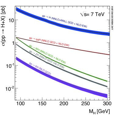
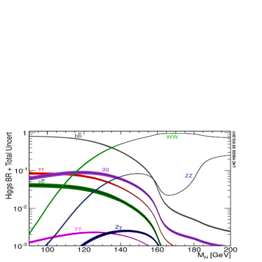
Figure 4: Predictions for SM Higgs boson cross sections at the LHC with $\sqrt{s}=7\,\,\mathrm{TeV}$ (left) and the decay branching ratios (right) YR1 ; YR2 . The central lines show the predictions, while the colored bands indicate the theoretical uncertainty.

2.4 Discovery of an SM Higgs-like particle at the LHC

On 4th of July 2012 both ATLAS ATLASdiscovery and CMS CMSdiscovery announced the discovery of a new boson with a mass of $\sim 125.5\,\,\mathrm{GeV}$. This discovery marks a milestone of an effort that has been ongoing for almost half a century and opens up a new era of particle physics. In Fig. 5 one can see the $p_{0}$ values of the search for the SM Higgs boson (with all search channels combined) as presented by ATLAS (left) and CMS (right) in July 2012. the $p_{0}$ value gives the probability that the experimental results observed can be caused by background only, i.e. in this case assuming the absense of a Higgs boson at each given mass. While the $p_{0}$ values are close to $\sim 0.5$ for nearly all hypothetical Higgs boson masses (as would be expected for the absense of a Higgs boson), both experiments show a very low $p_{0}$ value of $p_{0}\sim 10^{-6}$ around $M_{H}\sim 125.5\,\,\mathrm{GeV}$. This corresponds to a discovery of a new particle at the $5\,\sigma$ level by each experiment individually.

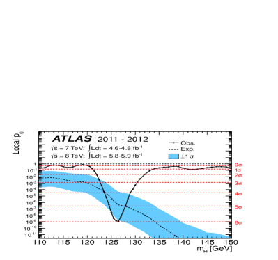
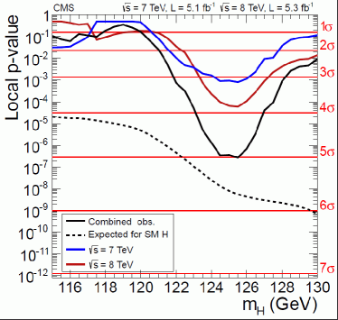
Figure 5: $p_{0}$ values in the SM Higgs boson search (all channels combined) as presented by ATLAS (left) ATLASdiscovery and CMS (right) CMSdiscovery on 4th of July 2012.

Another step in the analysis is a comparison of the measurement of production cross sectinos times branching ratios with the respective SM prediction, see Sect. 2.3. Two examples, using LHC data of about $5\mbox{fb}^{-1}$ at $7\,\,\mathrm{TeV}$ and about $12\mbox{fb}^{-1}$ at $8\,\,\mathrm{TeV}$ are shown in Fig. 6. Here ATLAS ATLAS_5p12ifb (left) and CMS CMS_5p12ifb (right) compare their experimental results with the SM prediction in various channels. It can be seen that all channels are, within the theoretical and experimental uncertainties, in agreement with the SM. However, it must be kept in mind that a measurement of the total width and thus of individual couplings is not possible at the LHC (see, e.g., Ref. lhc2tsp and references therein). Consequently, care must be taken in any coupling analysis. Recommendations of how these evaluations should be done using data from 2012 were given by the LHC Higgs Cross Section Working Group HiggsRecommendation .

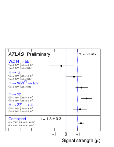
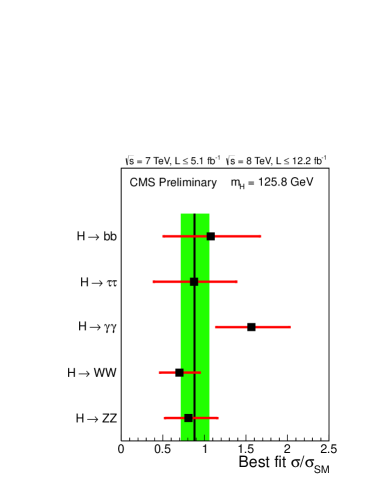
Figure 6: Comparison of the measurement of production cross sectinos times branching ratios with the respective SM prediction from ATLAS ATLAS_5p12ifb (left) and CMS CMS_5p12ifb (right).

2.5 Electroweak precision observables

Within the SM the electroweak precision observables (EWPO) have been used in particular to constrain the SM Higgs-boson mass $M_{H}^{\mathrm{SM}}$, before the discovery of the new boson at $\sim 125.5\,\,\mathrm{GeV}$. Originally the EWPO comprise over thousand measurements of “realistic observables” (with partially correlated uncertainties) such as cross sections, asymmetries, branching ratios etc. This huge set is reduced to 17 so-called “pseudo observables” by the LEP LEPEWWG and Tevatron TEVEWWG Electroweak working groups. The “pseudo observables” (again called EWPO in the following) comprise the $W$ boson mass $M_{W}$, the width of the $W$ boson, $\Gamma_{W}$, as well as various $Z$ pole observables: the effective weak mixing angle, $\sin^{2}\theta_{\mathrm{eff}}$, $Z$ decay widths to SM fermions, $\Gamma(Z\to f\bar{f})$, the invisible and total width, $\Gamma_{\rm inv}$ and $\Gamma_{Z}$, forward-backward and left-right asymmetries, $A_{\rm FB}^{f}$ and $A_{\rm LR}^{f}$, and the total hadronic cross section, $\sigma^{0}_{\rm had}$. The $Z$ pole results including their combination are final lepewwg . Experimental progress in recent years from the Tevatron comes for $M_{W}$ and $m_{t}$. (Also the error combination for $M_{W}$ and $\Gamma_{W}$ from the four LEP experiments has not been finalized yet due to not-yet-final analyses on the color-reconnection effects.)

The EWPO that give the strongest constraints on $M_{H}^{\mathrm{SM}}$ are $M_{W}$, $A_{\rm FB}^{b}$ and $A_{\rm LR}^{e}$. the value of $\sin^{2}\theta_{\mathrm{eff}}$ is extracted from a combination of various $A_{\rm FB}^{f}$ and $A_{\rm LR}^{f}$, where $A_{\rm FB}^{b}$ and $A_{\rm LR}^{e}$ give the dominant contribution.

The one-loop contributions to $M_{W}$ can be decomposed as follows sirlin ,

$$M_{W}^{2}\left(1-\frac{M_{W}^{2}}{M_{Z}^{2}}\right) =\frac{\pi\alpha}{\sqrt{2}G_{F}}\left(1+\Delta r\right),$$ (61)

$$\Delta r_{1-{\rm loop}} =\Delta\alpha-\frac{c_{\mathrm{w}}^{2}}{s_{\mathrm{w}}^{2}}\Delta\rho+\Delta r_{\rm rem}(M_{H}^{\mathrm{SM}}).$$ (62)

The first term, $\Delta\alpha$ contains large logarithmic contributions as $\log(M_{Z}/m_{f})$ and amounts $\sim 6\%$. the second term contains the $\rho$ parameter rho , being $\Delta\rho\sim m_{t}^{2}$. This term amounts $\sim 3.3\%$. The quantity $\Delta\rho$,

$$\Delta\rho =\frac{\Sigma^{Z}(0)}{M_{Z}^{2}}-\frac{\Sigma^{W}(0)}{M_{W}^{2}},$$ (63)

parameterizes the leading universal corrections to the electroweak precision observables induced by the mass splitting between fields in an isospin doublet. $\Sigma^{Z,W}(0)$ denote the transverse parts of the unrenormalized $Z$ and $W$ boson self-energies at zero momentum transfer, respectively. The final term in Eq. (62) is $\Delta r_{\rm rem}\sim\log(M_{H}^{\mathrm{SM}}/M_{W})$, and with a size of $\sim 1\%$ correction yields the constraints on $M_{H}^{\mathrm{SM}}$. the fact that the leading correction involving $M_{H}^{\mathrm{SM}}$ is logarithmic also applies to the other EWPO. Starting from two-loop order, also terms $\sim(M_{H}^{\mathrm{SM}}/M_{W})^{2}$ appear. the SM prediction of $M_{W}$ as a function of $m_{t}$ for the range $M_{H}^{\mathrm{SM}}=114\,\,\mathrm{GeV}\ldots 1000\,\,\mathrm{GeV}$ is shown as the dark shaded (green) band in Fig. 7 LEPEWWG , where an “intermediate region” of $M_{H}^{\mathrm{SM}}\sim 130\ldots 600\,\,\mathrm{GeV}$ as excluded by LHC SM Higgs searches is shown in yellow. the upper edge with $M_{H}^{\mathrm{SM}}=114\,\,\mathrm{GeV}$ corresponds to the (previous) lower limit on $M_{H}^{\mathrm{SM}}$ obtained at LEP LEPHiggsSM . the prediction is compared with the direct experimental result LEPEWWG ; mt1732 ,

$$M_{W}^{\rm exp} =80.385\pm 0.015\,\,\mathrm{GeV}~{},$$ (64)

$$m_{t}^{\rm exp} =173.2\pm 0.9\,\,\mathrm{GeV}~{},$$ (65)

shown as the solid (blue) ellipse (at the 68% CL) and with the indirect results for $M_{W}$ and $m_{t}$ as obtained from EWPO (dotted/red ellipse). The direct and indirect determination have significant overlap, representing a non-trivial success for the SM. Interpreting the newly discovered boson with a mass of $\sim 125.5\,\,\mathrm{GeV}$ as the SM Higgs boson, the plot shows agreement at the outer edge of the 68% CL ellipse. However, it should be noted that the experimental value of $M_{W}$ is somewhat higher than the region allowed by the LEP Higgs bounds: $M_{H}^{\mathrm{SM}}\approx 60\,\,\mathrm{GeV}$ is preferred as a central value by the measurement of $M_{W}$ and $m_{t}$.

  

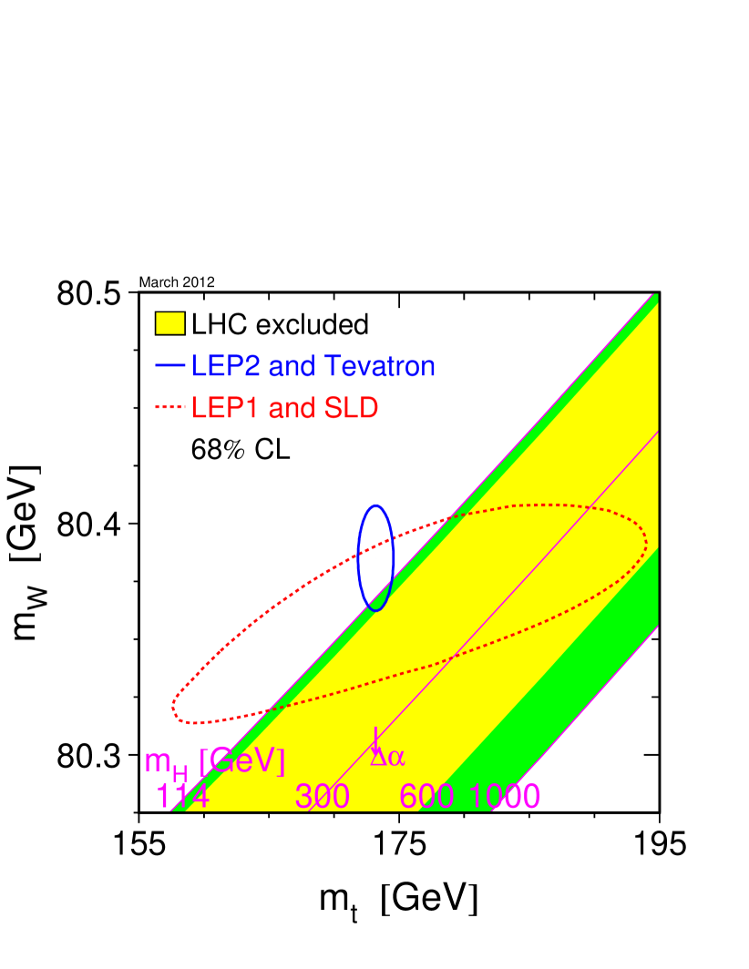
Figure 7: Prediction for $M_{W}$ in the SM as a function of $m_{t}$ for the range $M_{H}^{\mathrm{SM}}=114\,\,\mathrm{GeV}\ldots 1000\,\,\mathrm{GeV}$ LEPEWWG . The yellow area for the range $M_{H}^{\mathrm{SM}}\sim 130\ldots 600\,\,\mathrm{GeV}$ is exlcuded by LHC searches for the SM Higgs boson. The prediction is compared with the present experimental results for $M_{W}$ and $m_{t}$ (at the 68% CL) as well as with the indirect constraints obtained from EWPO.

The effective weak mixing angle is evaluated from various asymmetries and other EWPO as shown in Fig. 8 gruenewald07 (no update taking into account more recent $m_{t}$ measurements of this type of plot is availble). the average determination yields $\sin^{2}\theta_{\mathrm{eff}}=0.23153\pm 0.00016$ with a $\chi^{2}/{\rm d.o.f}$ of $11.8/5$, corresponding to a probability of $3.7\%$ gruenewald07 . the large $\chi^{2}$ is driven by the two single most precise measurements, $A_{\rm LR}^{e}$ by SLD and $A_{\rm FB}^{b}$ by LEP, where the earlier (latter) one prefers a value of $M_{H}^{\mathrm{SM}}\sim 32(437)\,\,\mathrm{GeV}$ gruenewaldpriv . The two measurements differ by more than $3\,\sigma$. The averaged value of $\sin^{2}\theta_{\mathrm{eff}}$, as shown in Fig. 8, prefers $M_{H}^{\mathrm{SM}}\sim 110\,\,\mathrm{GeV}$ gruenewaldpriv .

  

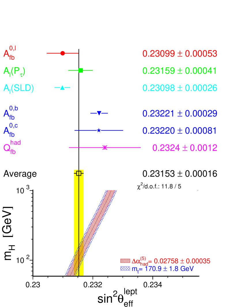
Figure 8: Prediction for $\sin^{2}\theta_{\mathrm{eff}}$ in the SM as a function of $M_{H}^{\mathrm{SM}}$ for $m_{t}=170.9\pm 1.8\,\,\mathrm{GeV}$ and $\Delta\alpha_{\rm had}^{5}=0.02758\pm 0.00035$ gruenewald07 . The prediction is compared with the present experimental results for $\sin^{2}\theta_{\mathrm{eff}}$ as averaged over several individual measurements.

The indirect $M_{H}^{\mathrm{SM}}$ determination for several individual EWPO is given in Fig. 9. Shown in the left plot are the central values of $M_{H}^{\mathrm{SM}}$ and the one $\sigma$ errors LEPEWWG . The dark shaded (green) vertical band indicates the combination of the various single measurements in the $1\,\sigma$ range. the vertical line shows the lower LEP bound for $M_{H}^{\mathrm{SM}}$ LEPHiggsSM . It can be seen that $M_{W}$, $A_{\rm LR}^{e}$ and $A_{\rm FB}^{b}$ give the most precise indirect $M_{H}^{\mathrm{SM}}$ determination, where only the latter one pulls the preferred $M_{H}^{\mathrm{SM}}$ value up, yielding a averaged value of LEPEWWG

$$M_{H}^{\mathrm{SM}}=94^{+29}_{-24}\,\,\mathrm{GeV}~{},$$ (66)

which would be in agreement with the discovery of a new boson at $\sim 125.5\,\,\mathrm{GeV}$. However, it is only the measurement of $A_{\rm FB}^{b}$ that yields the agreement of the SM with the new discovery.

The right plot in Fig. 9 shows similar results obtained by the GFitter group gfitter . Here also the experimental result for the SM Higgs seach is shown, indicating an approximate agreement of the indirect determination of $M_{H}^{\mathrm{SM}}$ with the experimental value.

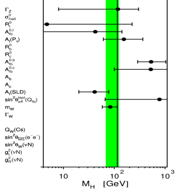
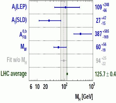
Figure 9: Indirect constrains on $M_{H}^{\mathrm{SM}}$ from various EWPO. Left: shown are the central values and the one $\sigma$ errors LEPEWWG . The dark shaded (green) vertical band indicates the combination of the various single measurements in the $1\,\sigma$ range. the vertical line shows the lower bound of $M_{H}^{\mathrm{SM}}\geq 114.4\,\,\mathrm{GeV}$ obtained at LEP LEPHiggsSM . Right: similar analysis by the GFitter group gfitter .

In Fig. 10 LEPEWWG we show the result for the global fit to $M_{H}^{\mathrm{SM}}$ including all EWPO, but not including the direct search bounds from LEP, the Tevatron and the LHC. $\Delta\chi^{2}$ is shown as a function of $M_{H}^{\mathrm{SM}}$, yielding Eq. (66) as best fit with an upper limit of $152\,\,\mathrm{GeV}$ at 95% CL. The theory (intrinsic) uncertainty in the SM calculations (as evaluated with TOPAZ0 topaz0 and ZFITTER zfitter ) are represented by the thickness of the blue band. the width of the parabola itself, on the other hand, is determined by the experimental precision of the measurements of the EWPO and the input parameters. Indicated as yellow areas are the $M_{H}^{\mathrm{SM}}$ values that are excluded by LEP and LHC searches, leaving only a small window of $M_{H}^{\mathrm{SM}}\sim 114\ldots 130\,\,\mathrm{GeV}$ open (reflecting that the plot was produced in March 2012). This window shrinks further taking into account the latest data from ATLAS ATLAS_5p12ifb and CMS CMS_5p12ifb . This plot demonstrates that a $\chi^{2}$ penalty of $\sim 1$ has to be paid to have $M_{H}^{\mathrm{SM}}\sim 125.5\,\,\mathrm{GeV}$ wrt. to the best fit value.

  

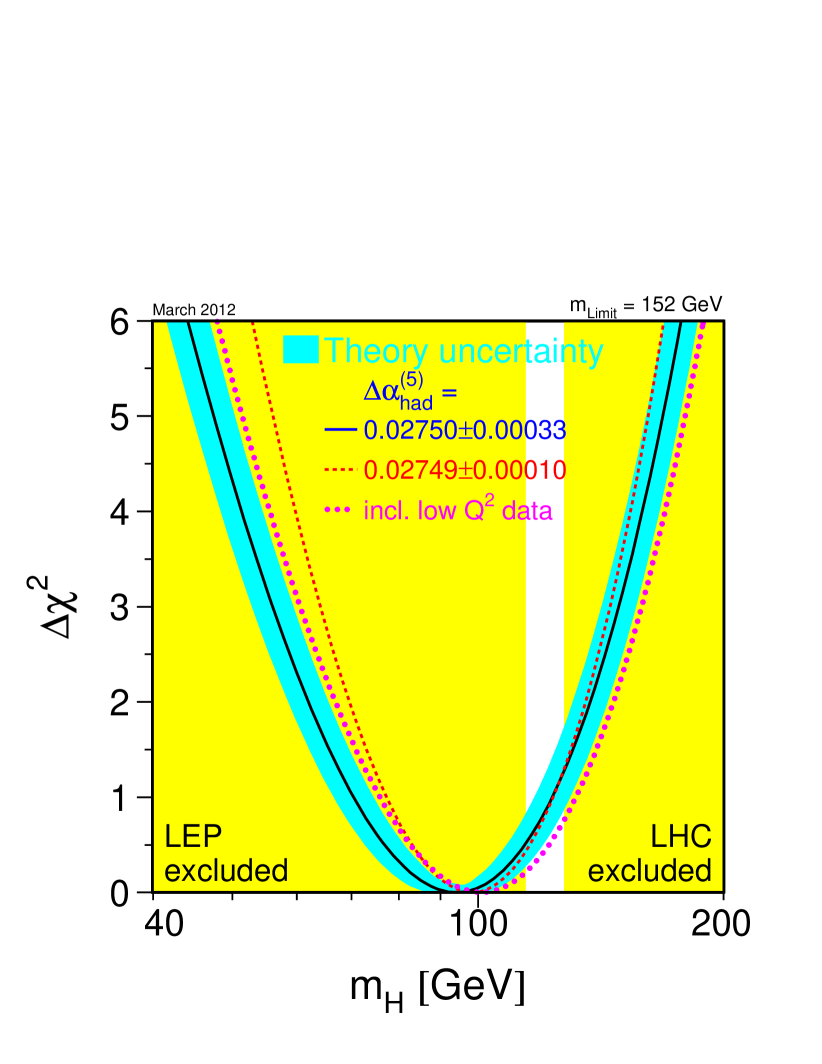
Figure 10: $\Delta\chi^{2}$ curve derived from all EWPO measured at LEP, SLD, CDF and D0, as a function of $M_{H}^{\mathrm{SM}}$, assuming the SM to be the correct theory of nature, and not including the direct bounds on $M_{H}^{\mathrm{SM}}$ LEPEWWG .

The current experimental uncertainties for the most relevant quantities, $\sin^{2}\theta_{\mathrm{eff}}$, $M_{W}$ and $m_{t}$ can be substantially improved at the ILC and in particular with the GigaZ option blueband ; gigaz ; moenig ; mwgigaz ; mtdet . It is expected that the leptonic weak effective mixing angle can be determined to $1.3\times 10^{-5}$, for the $W$ boson mass a precision of $7\,\,\mathrm{MeV}$ is expected, while for the top quark mass $0.1\,\,\mathrm{GeV}$ are anticipated from a precise determination of a well defined threshold mass. These improved accuracies will result in a substantially higher relative precision in the indirect determination of $M_{H}^{\mathrm{SM}}$, where with the GigaZ precision $\delta M_{H}^{\mathrm{SM}}/M_{H}^{\mathrm{SM}}\approx 16\%$ can be expected gruenewald07 . the comparison of the indirect $M_{H}^{\mathrm{SM}}$ determination with the direct measurement at the LHC atlas ; cms and the ILC Snowmass05Higgs ,

$$\delta M_{H}^{\mathrm{SM}}\mbox{}^{\rm,exp,LHC} \approx 200\,\,\mathrm{MeV},$$ (67)

$$\delta M_{H}^{\mathrm{SM}}\mbox{}^{\rm,exp,ILC} \approx 50\,\,\mathrm{MeV},$$ (68)

will constitute an important and profound consistency check of the model. This comparison will shed light on the basic theoretical components for generating the masses of the fundamental particles. On the other hand, an observed inconsistency would be a clear indication for the existence of a new physics scale.

3 The Higgs in Supersymmetry

3.1 Why SUSY?

Theories based on Supersymmetry (SUSY) mssm are widely considered as the theoretically most appealing extension of the SM. They are consistent with the approximate unification of the gauge coupling constants at the GUT scale and provide a way to cancel the quadratic divergences in the Higgs sector hence stabilizing the huge hierarchy between the GUT and the Fermi scales. Furthermore, in SUSY theories the breaking of the electroweak symmetry is naturally induced at the Fermi scale, and the lightest supersymmetric particle can be neutral, weakly interacting and absolutely stable, providing therefore a natural solution for the dark matter problem.

The Minimal Supersymmetric Standard Model (MSSM) constitutes, hence its name, the minimal supersymmetric extension of the SM. the number of SUSY generators is $N=1$, the smallest possible value. In order to keep anomaly cancellation, contrary to the SM a second Higgs doublet is needed glawei . All SM multiplets, including the two Higgs doublets, are extended to supersymmetric multiplets, resulting in scalar partners for quarks and leptons (“squarks” and “sleptons”) and fermionic partners for the SM gauge boson and the Higgs bosons (“gauginos”, “higgsinos” and “gluinos”). So far, the direct search for SUSY particles has not been successful. One can only set lower bounds of ${\cal O}(100\,\,\mathrm{GeV})$ to ${\cal O}(1000\,\,\mathrm{GeV})$ on their masses HCP2012 .

3.2 The MSSM Higgs sector

An excellent review on this subject is given in Ref. awb2 .

The Higgs boson sector at tree-level

Contrary to the Standard Model (SM), in the MSSM two Higgs doublets are required. The Higgs potential hhg

$$V =m_{1}^{2}|{\cal H}_{1}|^{2}+m_{2}^{2}|{\cal H}_{2}|^{2}-m_{12}^{2}(\epsilon_{ab}{\cal H}_{1}^{a}{\cal H}_{2}^{b}+\mbox{h.c.})$$

$$+\frac{1}{8}(g^{2}+g^{\prime 2})\left[|{\cal H}_{1}|^{2}-|{\cal H}_{2}|^{2}\right]^{2}+\frac{1}{2}g^{2}|{\cal H}_{1}^{{\dagger}}{\cal H}_{2}|^{2}~{},$$ (69)

contains $m_{1},m_{2},m_{12}$ as soft SUSY breaking parameters; $g,g^{\prime}$ are the $SU(2)$ and $U(1)$ gauge couplings, and $\epsilon_{12}=-1$.

The doublet fields ${\cal H}_{1}$ and ${\cal H}_{2}$ are decomposed in the following way:

$${\cal H}_{1} =\left(\begin{array}[]{c}{\cal H}_{1}^{0}\\[2.15277pt] {\cal H}_{1}^{-}\end{array}\right)\;=\;\left(\begin{array}[]{c}v_{1}+\frac{1}{\sqrt{2}}(\phi_{1}^{0}-i\chi_{1}^{0})\\[2.15277pt] -\phi_{1}^{-}\end{array}\right)~{},$$ (74)

$${\cal H}_{2} =\left(\begin{array}[]{c}{\cal H}_{2}^{+}\\[2.15277pt] {\cal H}_{2}^{0}\end{array}\right)\;=\;\left(\begin{array}[]{c}\phi_{2}^{+}\\[2.15277pt] v_{2}+\frac{1}{\sqrt{2}}(\phi_{2}^{0}+i\chi_{2}^{0})\end{array}\right)~{}.$$ (79)

${\cal H}_{1}$ gives mass to the down-type fermions, while ${\cal H}_{2}$ gives masses to the up-type fermions. The potential (69) can be described with the help of two independent parameters (besides $g$ and $g^{\prime}$): $\tan\beta=v_{2}/v_{1}$ and $M_{A}^{2}=-m_{12}^{2}(\tan\beta+\cot\beta)$, where $M_{A}$ is the mass of the ${\cal CP}$-odd Higgs boson $A$.

Which values can be expected for $\tan\beta$? One natural choice would be $\tan\beta\approx 1$, i.e. both vevs are about the same. On the other hand, one can argue that $v_{2}$ is responsible for the top quark mass, while $v_{1}$ gives rise to the bottom quark mass. Assuming that their mass differences comes largely from the vevs, while their Yukawa couplings could be about the same. the natural value for $\tan\beta$ would then be $\tan\beta\approx m_{t}/m_{b}$. Consequently, one can expect

$$1\;\raisebox{-3.00003pt}{$\stackrel{{\scriptstyle\displaystyle<}}{{\sim}}$}\;\tan\beta\;\raisebox{-3.00003pt}{$\stackrel{{\scriptstyle\displaystyle<}}{{\sim}}$}\;50~{}.$$ (80)

The diagonalization of the bilinear part of the Higgs potential, i.e. of the Higgs mass matrices, is performed via the orthogonal transformations

$$\left(\begin{array}[]{c}H^{0}\\[2.15277pt] h^{0}\end{array}\right) =\left(\begin{array}[]{cc}\cos\alpha&\sin\alpha\\[2.15277pt] -\sin\alpha&\cos\alpha\end{array}\right)\left(\begin{array}[]{c}\phi_{1}^{0}\\[2.15277pt] \phi_{2}^{0}~{},\end{array}\right)$$ (87)

$$\left(\begin{array}[]{c}G^{0}\\[2.15277pt] A^{0}\end{array}\right) =\left(\begin{array}[]{cc}\cos\beta&\sin\beta\\[2.15277pt] -\sin\beta&\cos\beta\end{array}\right)\left(\begin{array}[]{c}\chi_{1}^{0}\\[2.15277pt] \chi_{2}^{0}\end{array}\right)~{},$$ (94)

$$\left(\begin{array}[]{c}G^{\pm}\\[2.15277pt] H^{\pm}\end{array}\right) =\left(\begin{array}[]{cc}\cos\beta&\sin\beta\\[2.15277pt] -\sin\beta&\cos\beta\end{array}\right)\left(\begin{array}[]{c}\phi_{1}^{\pm}\\[2.15277pt] \phi_{2}^{\pm}\end{array}\right)~{}.$$ (101)

The mixing angle $\alpha$ is determined through

$$\alpha={\rm arctan}\left[\frac{-(M_{A}^{2}+M_{Z}^{2})\sin\beta\cos\beta}{M_{Z}^{2}\cos^{2}\!\beta+M_{A}^{2}\sin^{2}\!\beta-m^{2}_{h,{\rm tree}}}\right]~{},~{}~{}-\frac{\pi}{2}<\alpha<0$$ (102)

with $m_{h,{\rm tree}}$ defined below in Eq. (113).
One gets the following Higgs spectrum:

$$\mbox{2 neutral bosons},\,{\cal CP}=+1 :h,H$$

$$\mbox{1 neutral boson},\,{\cal CP}=-1 :A$$

2 charged bosons $$:H^{+},H^{-}$$

3 unphysical Goldstone bosons $$:G,G^{+},G^{-}.$$ (103)

At tree level the mass matrix of the neutral ${\cal CP}$-even Higgs bosons is given in the $\phi_{1}$-$\phi_{2}$-basis in terms of $M_{Z}$, $M_{A}$, and $\tan\beta$ by

$$M_{\rm Higgs}^{2,{\rm tree}} =\left(\begin{array}[]{cc}m_{\phi_{1}}^{2}&m_{\phi_{1}\phi_{2}}^{2}\\ m_{\phi_{1}\phi_{2}}^{2}&m_{\phi_{2}}^{2}\end{array}\right)$$ (106)

$$=\left(\begin{array}[]{cc}M_{A}^{2}\sin^{2}\!\beta+M_{Z}^{2}\cos^{2}\!\beta&-(M_{A}^{2}+M_{Z}^{2})\sin\beta\cos\beta\\ -(M_{A}^{2}+M_{Z}^{2})\sin\beta\cos\beta&M_{A}^{2}\cos^{2}\!\beta+M_{Z}^{2}\sin^{2}\!\beta\end{array}\right),$$ (109)

which by diagonalization according to Eq. (87) yields the tree-level Higgs boson masses

$$M_{\rm Higgs}^{2,{\rm tree}}\stackrel{{\scriptstyle\alpha}}{{\longrightarrow}}\left(\begin{array}[]{cc}m_{H,{\rm tree}}^{2}&0\\ 0&m_{h,{\rm tree}}^{2}\end{array}\right)$$ (112)

with

$$m_{H,h,{\rm tree}}^{2} =\tfrac{1}{2}\left[M_{A}^{2}+M_{Z}^{2}\pm\sqrt{(M_{A}^{2}+M_{Z}^{2})^{2}-4M_{Z}^{2}M_{A}^{2}\cos^{2}2\beta}\right]~{}.$$ (113)

From this formula the famous tree-level bound

$$m_{h,{\rm tree}}\leq\mbox{min}\{M_{A},M_{Z}\}\cdot|\cos 2\beta|\leq M_{Z}$$ (114)

can be obtained. The charged Higgs boson mass is given by

$$m_{H^{\pm}}^{2}=M_{A}^{2}+M_{W}^{2}~{}.$$ (115)

The masses of the gauge bosons are given in analogy to the SM:

$$M_{W}^{2}=\frac{1}{2}g^{2}(v_{1}^{2}+v_{2}^{2});\qquad M_{Z}^{2}=\frac{1}{2}(g^{2}+g^{\prime 2})(v_{1}^{2}+v_{2}^{2});\qquad M_{\gamma}=0.$$ (116)

The couplings of the Higgs bosons are modified from the corresponding SM couplings already at the tree-level. Some examples are

$$g_{hVV} =\sin(\beta-\alpha)\;g_{HVV}^{\rm SM},\quad V=W^{\pm},Z~{},$$ (117)

$$g_{HVV} =\cos(\beta-\alpha)\;g_{HVV}^{\rm SM}~{},$$ (118)

$$g_{hb\bar{b}},g_{h\tau^{+}\tau^{-}} =-\frac{\sin\alpha}{\cos\beta}\;g_{Hb\bar{b},H\tau^{+}\tau^{-}}^{\rm SM}~{},$$ (119)

$$g_{ht\bar{t}} =\frac{\cos\alpha}{\sin\beta}\;g_{Ht\bar{t}}^{\rm SM}~{},$$ (120)

$$g_{Ab\bar{b}},g_{A\tau^{+}\tau^{-}} =\gamma_{5}\tan\beta\;g_{Hb\bar{b},H\tau^{+}\tau^{-}}^{\rm SM}~{}.$$ (121)

The following can be observed: the couplings of the ${\cal CP}$-even Higgs boson to SM gauge bosons is always suppressed with respect to the SM coupling. However, if $g_{hVV}^{2}$ is close to zero, $g_{HVV}^{2}$ is close to $(g_{HVV}^{\rm SM})^{2}$ and vice versa, i.e. it is not possible to decouple both of them from the SM gauge bosons. The coupling of the $h$ to down-type fermions can be suppressed or enhanced with respect to the SM value, depending on the size of $\sin\alpha/\cos\beta$. Especially for not too large values of $M_{A}$ and large $\tan\beta$ one finds $|\sin\alpha/\cos\beta|\gg 1$, leading to a strong enhancement of this coupling. the same holds, in principle, for the coupling of the $h$ to up-type fermions. However, for large parts of the MSSM parameter space the additional factor is found to be $|\cos\alpha/\sin\beta|<1$. For the ${\cal CP}$-odd Higgs boson an additional factor $\tan\beta$ is found. According to Eq. (80) this can lead to a strongly enhanced coupling of the $A$ boson to bottom quarks or $\tau$ leptons, resulting in new search strategies at the Tevatron and the LHC for the ${\cal CP}$-odd Higgs boson, see Sect. 3.3.

For $M_{A}\;\raisebox{-3.00003pt}{$\stackrel{{\scriptstyle\displaystyle>}}{{\sim}}$}\;150\,\,\mathrm{GeV}$ the “decoupling limit” is reached. The couplings of the light Higgs boson become SM-like, i.e. the additional factors approach 1. the couplings of the heavy neutral Higgs bosons become similar, $g_{Axx}\approx g_{Hxx}$, and the masses of the heavy neutral and charged Higgs bosons fulfill $M_{A}\approx M_{H}\approx M_{H^{\pm}}$. As a consequence, search strategies for the $A$ boson can also be applied to the $H$ boson, and both are hard to disentangle at hadron colliders (see also Fig. 11 below).

The scalar quark sector

Since the most relevant squarks for the MSSM Higgs boson sector are the $\tilde{t}$ and $\tilde{b}$ particles, here we explicitly list their mass matrices in the basis of the gauge eigenstates $\tilde{t}_{L},\tilde{t}_{R}$ and $\tilde{b}_{L},\tilde{b}_{R}$:

$${\cal M}^{2}_{\tilde{t}} =\left(\begin{array}[]{cc}M_{\tilde{t}_{L}}^{2}+m_{t}^{2}+\cos 2\beta(\tfrac{1}{2}-\frac{2}{3}s_{\mathrm{w}}^{2})M_{Z}^{2}&m_{t}X_{t}\\ m_{t}X_{t}&M_{\tilde{t}_{R}}^{2}+m_{t}^{2}+\frac{2}{3}\cos 2\beta s_{\mathrm{w}}^{2}M_{Z}^{2}\end{array}\right),$$ (124)

$${\cal M}^{2}_{\tilde{b}} =\left(\begin{array}[]{cc}M_{\tilde{b}_{L}}^{2}+m_{b}^{2}+\cos 2\beta(-\tfrac{1}{2}+\frac{1}{3}s_{\mathrm{w}}^{2})M_{Z}^{2}&m_{b}X_{b}\\ m_{b}X_{b}&M_{\tilde{b}_{R}}^{2}+m_{b}^{2}-\frac{1}{3}\cos 2\beta s_{\mathrm{w}}^{2}M_{Z}^{2}\end{array}\right).$$ (127)

$M_{\tilde{t}_{L}}$, $M_{\tilde{t}_{R}}$, $M_{\tilde{b}_{L}}$ and $M_{\tilde{b}_{R}}$ are the (diagonal) soft SUSY-breaking parameters. We furthermore have

$$m_{t}X_{t}=m_{t}(A_{t}-\mu\cot\beta),\quad m_{b}\,X_{b}=m_{b}\,(A_{b}-\mu\tan\beta).$$ (128)

The soft SUSY-breaking parameters $A_{t}$ and $A_{b}$ denote the trilinear Higgs–stop and Higgs–sbottom coupling, and $\mu$ is the Higgs mixing parameter. $SU(2)$ gauge invariance requires the relation

$$M_{\tilde{t}_{L}}=M_{\tilde{b}_{L}}.$$ (129)

Diagonalizing ${\cal M}^{2}_{\tilde{t}}$ and ${\cal M}^{2}_{\tilde{b}}$ with the mixing angles $\theta_{\tilde{t}}$ and $\theta_{\tilde{b}}$, respectively, yields the physical $\tilde{t}$ and $\tilde{b}$ masses: $m_{\tilde{t}_{1}}$, $m_{\tilde{t}_{2}}$, $m_{\tilde{b}_{1}}$ and $m_{\tilde{b}_{2}}$.

Higher-order corrections to Higgs boson masses

A review about this subject can be found in Ref. habilSH . In the Feynman diagrammatic (FD) approach the higher-order corrected ${\cal CP}$-even Higgs boson masses in the rMSSM are derived by finding the poles of the $(h,H)$-propagator matrix. the inverse of this matrix is given by

$$\left(\Delta_{\rm Higgs}\right)^{-1}=-i\left(\begin{array}[]{cc}p^{2}-m_{H,{\rm tree}}^{2}+\hat{\Sigma}_{HH}(p^{2})&\hat{\Sigma}_{hH}(p^{2})\\ \hat{\Sigma}_{hH}(p^{2})&p^{2}-m_{h,{\rm tree}}^{2}+\hat{\Sigma}_{hh}(p^{2})\end{array}\right)~{}.$$ (130)

Determining the poles of the matrix $\Delta_{\rm Higgs}$ in Eq. (130) is equivalent to solving the equation

$$\left[p^{2}-m_{h,{\rm tree}}^{2}+\hat{\Sigma}_{hh}(p^{2})\right]\left[p^{2}-m_{H,{\rm tree}}^{2}+\hat{\Sigma}_{HH}(p^{2})\right]-\left[\hat{\Sigma}_{hH}(p^{2})\right]^{2}=0\,.$$ (131)

The very leading one-loop correction to $M_{h}^{2}$ is given by

$$\Delta M_{h}^{2} =G_{F}m_{t}^{4}\log\left(\frac{m_{\tilde{t}_{1}}m_{\tilde{t}_{2}}}{m_{t}^{2}}\right)~{},$$ (132)

where $G_{F}$ denotes the Fermi constant. the Eq. (132) shows two important aspects: First, the leading loop corrections go with $m_{t}^{4}$, which is a “very large number”. Consequently, the loop corrections can strongly affect $M_{h}$ and pushed the mass beyond the reach of LEP LEPHiggsSM ; LEPHiggsMSSM and into the mass regime of the newly discovered boson at $\sim 125.5\,\,\mathrm{GeV}$. Second, the scalar fermion masses (in this case the scalar top masses) appear in the log entering the loop corrections (acting as a “cut-off” where the new physics enter). In this way the light Higgs boson mass depends on all other sectors via loop corrections. This dependence is particularly pronounced for the scalar top sector due to the large mass of the top quark.

The status of the available results for the self-energy contributions to Eq. (130) can be summarized as follows. For the one-loop part, the complete result within the MSSM is known ERZ ; mhiggsf1lA ; mhiggsf1lB ; mhiggsf1lC . the by far dominant one-loop contribution is the ${\cal O}(\alpha_{t})$ term due to top and stop loops, see also Eq. (132), ($\alpha_{t}\equiv h_{t}^{2}/(4\pi)$, $h_{t}$ being the superpotential top coupling). Concerning the two-loop effects, their computation is quite advanced and has now reached a stage such that all the presumably dominant contributions are known. They include the strong corrections, usually indicated as ${\cal O}(\alpha_{t}\alpha_{s})$, and Yukawa corrections, ${\cal O}(\alpha_{t}^{2})$, to the dominant one-loop ${\cal O}(\alpha_{t})$ term, as well as the strong corrections to the bottom/sbottom one-loop ${\cal O}(\alpha_{b})$ term ($\alpha_{b}\equiv h_{b}^{2}/(4\pi)$), i.e. the ${\cal O}(\alpha_{b}\alpha_{s})$ contribution. The latter can be relevant for large values of $\tan\beta$. Presently, the ${\cal O}(\alpha_{t}\alpha_{s})$ mhiggsEP1b ; mhiggsletter ; mhiggslong ; mhiggsEP0 ; mhiggsEP1 , ${\cal O}(\alpha_{t}^{2})$ mhiggsEP1b ; mhiggsEP3 ; mhiggsEP2 and the ${\cal O}(\alpha_{b}\alpha_{s})$ mhiggsEP4 ; mhiggsFD2 contributions to the self-energies are known for vanishing external momenta. In the (s)bottom corrections the all-order resummation of the $\tan\beta$-enhanced terms, ${\cal O}(\alpha_{b}(\alpha_{s}\tan\beta)^{n})$ and ${\cal O}(\alpha_{b}(\alpha_{t}\tan\beta)^{n})$, is also performed deltamb1 ; deltamb . The ${\cal O}(\alpha_{t}\alpha_{b})$ and ${\cal O}(\alpha_{b}^{2})$ corrections were presented in Ref. mhiggsEP4b . A “nearly full” two-loop effective potential calculation (including even the momentum dependence for the leading pieces and the leading three-loop corrections) has been published mhiggsEP5 . Most recently another leading three-loop calculation, valid for certain SUSY mass combinations, became available mhiggsFD3l . The remaining theoretical uncertainty on the lightest ${\cal CP}$-even Higgs boson mass has been estimated to be of $\sim 3\,\,\mathrm{GeV}$ mhiggsAEC ; PomssmRep . Taking the available loop corrections into account, the upper limit of $M_{h}$ is shifted to mhiggsAEC ,

$$M_{h}\leq 135\,\,\mathrm{GeV}~{}$$ (133)

(as obtained with the code FeynHiggs feynhiggs ; mhiggslong ; mhiggsAEC ; mhcMSSMlong ). This limit takes into account the experimental uncertainty for the top quark mass, see Eq. (65), as well as the intrinsic uncertainties from unknown higher-order corrections. Consequently, a Higgs boson with a mass of $\sim 125.5\,\,\mathrm{GeV}$ can naturally be explained by the MSSM. Either the light or the heavy ${\cal CP}$-even Higgs boson can be interpreted as the newly discovered particle, which will be discussed in more detail in Sect. 3.4.

The charged Higgs boson mass is obtained by solving the equation

$$p^{2}-m_{H^{\pm}}^{2}-\hat{\Sigma}_{H^{-}H^{+}}(p^{2})=0~{}.$$ (134)

The charged Higgs boson self-energy is known at the one-loop level chargedmhiggs ; markusPhD .

3.3 MSSM Higgs bosons at the LHC

The “decoupling limit” has been discussed for the tree-level couplings and masses of the MSSM Higgs bosons in Sect. 3.2. This limit also persists taking into account radiative corrections. the corresponding Higgs boson masses are shown in Fig. 11 for $\tan\beta=5$ in the $m_{h}^{\rm max}$ benchmark scenario benchmark2 obtained with FeynHiggs. For $M_{A}\;\raisebox{-3.00003pt}{$\stackrel{{\scriptstyle\displaystyle>}}{{\sim}}$}\;180\,\,\mathrm{GeV}$ the lightest Higgs boson mass approaches its upper limit (depending on the SUSY parameters), and the heavy Higgs boson masses are nearly degenerate. Furthermore, also the light Higgs boson couplings including loop corrections approach their SM-value for. Consequently, for $M_{A}\;\raisebox{-3.00003pt}{$\stackrel{{\scriptstyle\displaystyle>}}{{\sim}}$}\;180\,\,\mathrm{GeV}$ an SM-like Higgs boson (below $\sim 135\,\,\mathrm{GeV}$) can naturally be explained by the MSSM. On the other hand, deviations from a SM-like behavior can be described in the MSSM by deviating from the full decoupling limit.

  

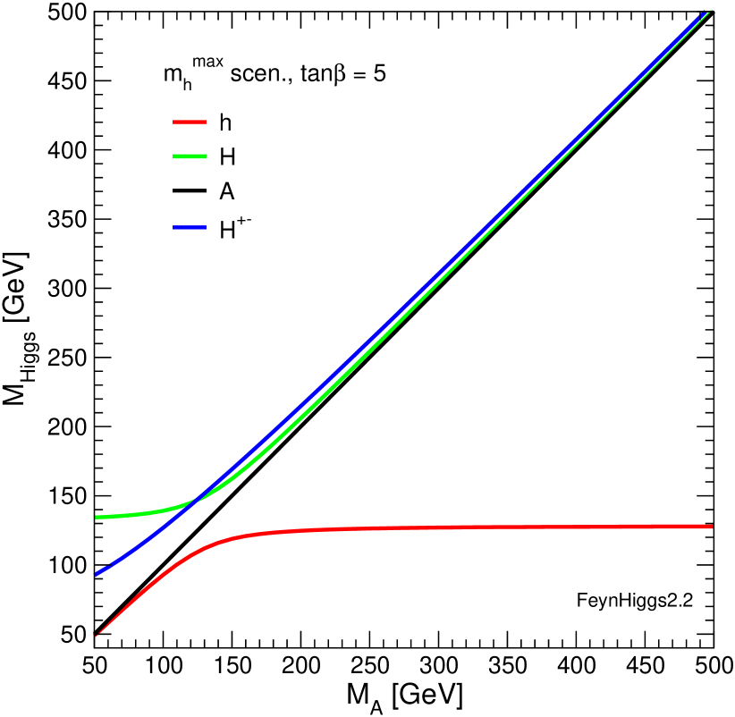
Figure 11: The MSSM Higgs boson masses including higher-order corrections are shown as a function of $M_{A}$ for $\tan\beta=5$ in the $m_{h}^{\rm max}$ benchmark scenario benchmark2 (obtained with FeynHiggs feynhiggs ; mhiggslong ; mhiggsAEC ; mhcMSSMlong ).

An example for the various productions cross sections at the LHC is shown in Fig. 12 (for $\sqrt{s}=14\,\,\mathrm{TeV}$). For low masses the light Higgs cross sections are visible, and for $M_{H}\;\raisebox{-3.00003pt}{$\stackrel{{\scriptstyle\displaystyle>}}{{\sim}}$}\;130\,\,\mathrm{GeV}$ the heavy ${\cal CP}$-even Higgs cross section is displayed, while the cross sections for the ${\cal CP}$-odd $A$ boson are given for the whole mass range. As discussed in Sect. 3.2 the $g_{Abb}$ coupling is enhanced by $\tan\beta$ with respect to the corresponding SM value. Consequently, the $b\bar{b}A$ cross section is the largest or second largest cross section for all $M_{A}$, despite the relatively small value of $\tan\beta=5$. For larger $\tan\beta$, see Eq. (80), this cross section can become even more dominant. Furthermore, the coupling of the heavy ${\cal CP}$-even Higgs boson becomes very similar to the one of the $A$ boson, and the two production cross sections, $b\bar{b}A$ and $b\bar{b}H$ are indistinguishable in the plot for $M_{A}>200\,\,\mathrm{GeV}$.

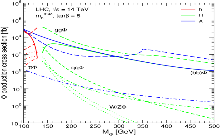
Figure 12: Overview about the various neutral Higgs boson production cross sections at the LHC shown as a function of $M_{A}$ for $\tan\beta=5$ in the $m_{h}^{\rm max}$ scenario (taken from Ref. sigmaH , where the original references can be found).

More precise results in the most important channels, $gg\to\phi$ and $b\bar{b}\to\phi$ ($\phi=h,H,A$) have been obtained by the LHC Higgs Cross Section Working Group lhchxswg , see also Refs. YR1 ; YR2 and references therein. Most recently a new code, SusHi sushi for the $gg\to\phi$ production mode including the full MSSM one-loop contributions as well as higher-order SM and MSSM corrections has been presented, see Ref. gghMSSM for more details.

Following the above discussion, the main search channel for heavy Higgs bosons at the LHC for $M_{A}\;\raisebox{-3.00003pt}{$\stackrel{{\scriptstyle\displaystyle>}}{{\sim}}$}\;200\,\,\mathrm{GeV}$ is the production in association with bottom quarks and the subsequent decay to tau leptons, $b\bar{b}\to b\bar{b}\;H/A\to b\bar{b}\;\tau^{+}\tau^{-}$. For heavy supersymmetric particles, with masses far above the Higgs boson mass scale, one has for the production and decay of the $A$ boson benchmark3

$$\sigma(b\bar{b}A)\times{\rm BR}(A\to b\bar{b})\simeq\sigma(b\bar{b}H)_{\rm SM}\;\frac{\tan^{2}\beta}{\left(1+\Delta_{b}\right)^{2}}\times\frac{9}{\left(1+\Delta_{b}\right)^{2}+9}~{},$$ (135)

$$\sigma(gg,b\bar{b}\to A)\times{\rm BR}(A\to\tau^{+}\tau^{-})\simeq\sigma(gg,b\bar{b}\to H)_{\rm SM}\;\frac{\tan^{2}\beta}{\left(1+\Delta_{b}\right)^{2}+9}~{},$$ (136)

where $\sigma(b\bar{b}H)_{\rm SM}$ and $\sigma(gg,b\bar{b}\to H)_{\rm SM}$ denote the values of the corresponding SM Higgs boson production cross sections for $M_{H}^{\mathrm{SM}}=M_{A}$. The leading contributions to $\Delta_{b}$ are given by deltamb1

$$\Delta_{b}\approx\frac{2\alpha_{s}}{3\,\pi}\,m_{\tilde{g}}\,\mu\,\tan\beta\,\times\,I(m_{\tilde{b}_{1}},m_{\tilde{b}_{2}},m_{\tilde{g}})+\frac{\alpha_{t}}{4\,\pi}\,A_{t}\,\mu\,\tan\beta\,\times\,I(m_{\tilde{t}_{1}},m_{\tilde{t}_{2}},|\mu|)~{},$$ (137)

where the function $I$ arises from the one-loop vertex diagrams and scales as $I(a,b,c)\sim 1/\mbox{max}(a^{2},b^{2},c^{2})$. Here $m_{\tilde{g}}$ is the gluino mass, and $\mu$ is the Higgs mixing parameter. As a consequence, the $b\bar{b}$ production rate depends sensitively on $\Delta_{b}\propto\mu\,\tan\beta$ because of the factor $1/(1+\Delta_{b})^{2}$, while this leading dependence on $\Delta_{b}$ cancels out in the $\tau^{+}\tau^{-}$ production rate. The formulas above apply, within a good approximation, also to the heavy ${\cal CP}$-even Higgs boson in the large $\tan\beta$ regime. Therefore, the production and decay rates of $H$ are governed by similar formulas as the ones given above, leading to an approximate enhancement by a factor 2 of the production rates with respect to the ones that would be obtained in the case of the single production of the ${\cal CP}$-odd Higgs boson as given in Eqs. (135), (136).

Of particular interest is the “LHC wedge” region, i.e. the region in which only the light ${\cal CP}$-even MSSM Higgs boson, but none of the heavy MSSM Higgs bosons can be detected at the LHC. It appears for $M_{A}\;\raisebox{-3.00003pt}{$\stackrel{{\scriptstyle\displaystyle>}}{{\sim}}$}\;200\,\,\mathrm{GeV}$ at intermediate $\tan\beta$ and widens to larger $\tan\beta$ values for larger $M_{A}$. Consequently, in the “LHC wedge” only a SM-like light Higgs boson can be discovered at the LHC, and part of the LHC wedge (depending on the explicit choice of SUSY parameters) can be in agreement with $M_{h}\sim 125.5\,\,\mathrm{GeV}$. This region, bounded from above by the 95% CL exclusion contours for the heavy neutral MSSM Higgs bosons can be seen in Fig. 13 CMS-HAtautau . Here it should be kept in mind that the actual position of the exlcusion contour depends on $\Delta_{b}$ and thus on the sign and the size of $\mu$ as discussed above.

  

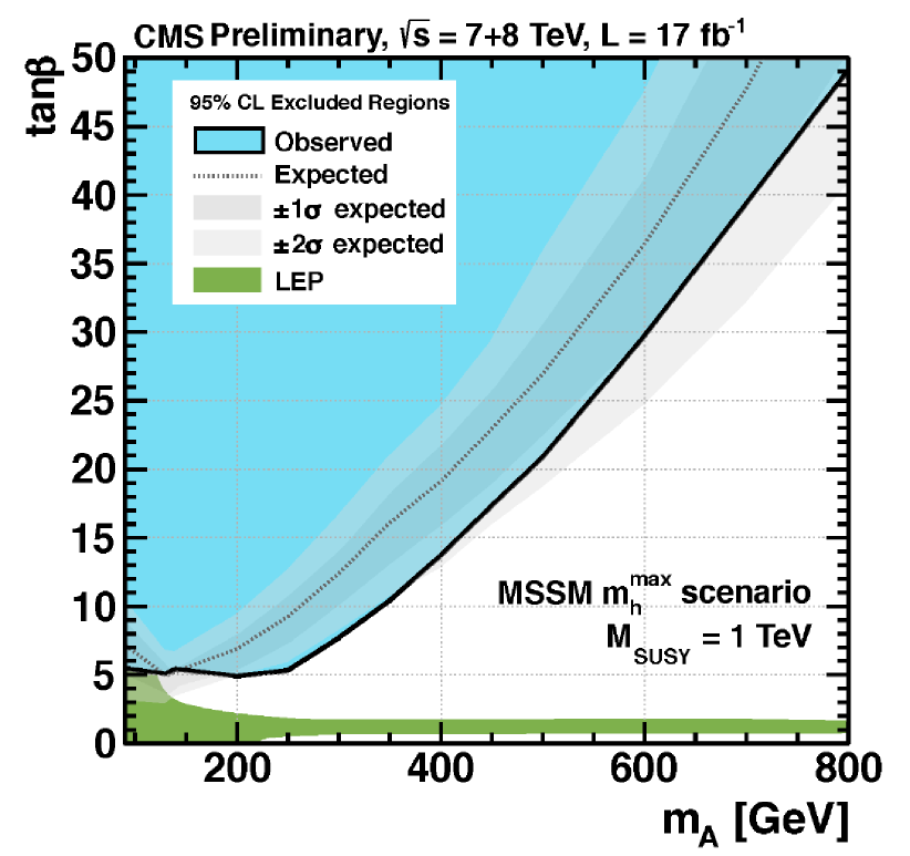
Figure 13: The 95% CL exclusion regions (i.e. the upper bound of the “LHC wedge” region) for the heavy neutral Higgs bosons in the channel $pp\to H/A\to\tau^{+}\tau^{-}(+X)$, obtained by CMS including $\sqrt{s}=7,8\,\,\mathrm{TeV}$ data CMS-HAtautau .

3.4 Agreement of the MSSM Higgs sector with
       a Higgs at $\sim 125.5\,\,\mathrm{GeV}$

Many investigations have been performed analyzing the agreement of the MSSM with a Higgs boson at $\sim 125.5\,\,\mathrm{GeV}$. In a first step only the mass information can be used to test the model, while in a second step also the rate information of the various Higgs search channels can be taken into account. Here we briefly review the first MSSM results Mh125 that were published after the first ATLAS/CMS announcement in December 2012 Dec13 (see Refs. Mh125-gaga ; hifi for updates of these results, including rate analyses, and for an extensive list of references).

In the left plot of Fig. 14 Mh125 the $M_{A}$-$\tan\beta$ plane in the $m_{h}^{\rm max}$ benchmark scenario benchmark2 is shown, where the area in light and dark green yield a mass for the light ${\cal CP}$-even Higgs around $\sim 125.5\,\,\mathrm{GeV}$. The brown area is excluded by LHC heavy MSSM Higgs boson searches in the $H/A\to\tau\tau$ channel (although not the latest results as presented in Ref. CMS-HAtautau ), the blue area is excluded by LEP Higgs searches LEPHiggsSM ; LEPHiggsMSSM . (The limits have been obtained with HiggsBounds higgsbounds version 3.5.0-beta). Since the $m_{h}^{\rm max}$ scenario maximizes the light ${\cal CP}$-even Higgs boson mass it is possible to extract lower (one parameter) limits on $M_{A}$ and $\tan\beta$ from the edges of the green band. By choosing the parameters entering via radiative corrections such that those corrections yield a maximum upward shift to $M_{h}$, the lower bounds on $M_{A}$ and $\tan\beta$ that can be obtained are general in the sense that they (approximately) hold for any values of the other parameters. To address the (small) residual $M_{\rm SUSY}(:=M_{\tilde{t}_{L}}=M_{\tilde{t}_{R}}=M_{\tilde{b}_{R}})$ dependence of the lower bounds on $M_{A}$ and $\tan\beta$, limits have been extracted for the three different values $M_{\rm SUSY}=\{0.5,1,2\}\,\,\mathrm{TeV}$, see Tab. 1. For comparison also the previous limits derived from the LEP Higgs searches LEPHiggsMSSM are shown, i.e. before the incorporation of the new LHC results reported in Ref. Dec13 . The bounds on $M_{A}$ translate directly into lower limits on $M_{H^{\pm}}$, which are also given in the table. A phenomenological consequence of the bound $M_{H^{\pm}}\;\raisebox{-3.00003pt}{$\stackrel{{\scriptstyle\displaystyle>}}{{\sim}}$}\;155\,\,\mathrm{GeV}$ (for $M_{\rm SUSY}=1\,\,\mathrm{TeV}$) is that it would leave only a very small kinematic window open for the possibility that MSSM charged Higgs bosons are produced in the decay of top quarks.

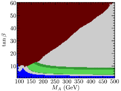
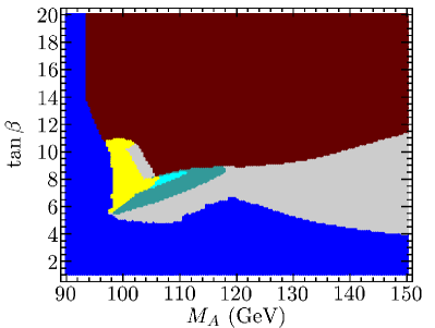
Figure 14: Left: $M_{A}$-$\tan\beta$ plane in the $m_{h}^{\rm max}$ scenario; the green shaded area yields $M_{h}\sim 125.5\,\,\mathrm{GeV}$, the brown area is excluded by LHC heavy MSSM Higgs boson searches, the blue area is excluded by LEP Higgs searches. Right: $M_{A}$-$\tan\beta$ plane with $M_{\rm SUSY}=\mu=1\,\,\mathrm{TeV}$, $X_{t}=2.3\,\,\mathrm{TeV}$; the yellow area yields $M_{H}\sim 125.5\,\,\mathrm{GeV}$ with an SM-like heavy ${\cal CP}$-even Higgs boson, brown and blue areas are excluded by LHC and LEP Higgs searches, respectively Mh125 .

	Limits without $M_{h}\sim 125\,\,\mathrm{GeV}$			Limits with $M_{h}\sim 125\,\,\mathrm{GeV}$
$M_{\rm SUSY}$ (GeV)	$\tan\beta$	$M_{A}$ (GeV)	$M_{H^{\pm}}$ (GeV)	$\tan\beta$	$M_{A}$ (GeV)	$M_{H^{\pm}}$ (GeV)
500	$2.7$	$95$	$123$	$4.5$	$140$	$161$
1000	$2.2$	$95$	$123$	$3.2$	$133$	$155$
2000	$2.0$	$95$	$123$	$2.9$	$130$	$152$

Table 1: Lower limits on the MSSM Higgs sector tree-level parameters $M_{A}$ ($M_{H^{\pm}}$) and $\tan\beta$ obtained with and without the assumed Higgs signal of $M_{h}\sim 125.5\,\,\mathrm{GeV}$. the mass limits have been rounded to $1\,\,\mathrm{GeV}$ Mh125 .

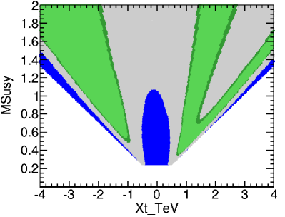
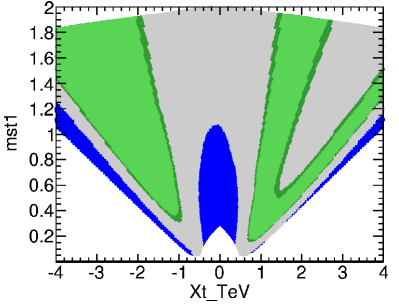
Figure 15: Scalar top masses in the $m_{h}^{\rm max}$ scenario (with $M_{\rm SUSY}$ and $X_{t}$ free) that yield $M_{h}\sim 125.5\,\,\mathrm{GeV}$ (green area), LEP excluded regions are shown in blue. Left: $X_{t}$-$M_{\rm SUSY}$ plane, right: $X_{t}$-$m_{\tilde{t}_{1}}$ plane Mh125 .

It is also possible to investigate what can be inferred from the assumed Higgs signal about the higher-order corrections in the Higgs sector. Similarly to the previous case, one can obtain an absolute lower limit on the stop mass scale $M_{\rm SUSY}$ by considering the maximal tree-level contribution to $M_{h}$. The resulting constraints for $M_{\rm SUSY}$ and $X_{t}$, obtaind in the decoupling limit for $M_{A}=1\,\,\mathrm{TeV}$ and $\tan\beta=20$, are shown in the left plot of Fig. 15 Mh125 with the same colour coding as before. Several favoured branches develop in this plane, centred around $X_{t}\sim-1.5M_{\rm SUSY}$, $X_{t}\sim 1.2M_{\rm SUSY}$, and $X_{t}\sim 2.5M_{\rm SUSY}$. The minimal allowed stop mass scale is $M_{\rm SUSY}\sim 300\,\,\mathrm{GeV}$ with positive $X_{t}$ and $M_{\rm SUSY}\sim 500\,\,\mathrm{GeV}$ for negative $X_{t}$. The results on the stop sector can also be interpreted as a lower limit on the mass $m_{\tilde{t}_{1}}$ of the lightest stop squark. This is shown in the right plot of Fig. 15. Interpreting the newly observed particle as the light ${\cal CP}$-even Higgs one obtains the lower bounds $m_{\tilde{t}_{1}}>100\,\,\mathrm{GeV}$ ($X_{t}>0$) and $m_{\tilde{t}_{1}}>250\,\,\mathrm{GeV}$ ($X_{t}<0$).

Finally, in the right plot of Fig. 14 Mh125 it is demonstrated that also the heavy ${\cal CP}$-even Higgs can be interpreted as the newly discovered particle at $\sim 125.5\,\,\mathrm{GeV}$. the $M_{A}$-$\tan\beta$ plane is shown for $M_{\rm SUSY}=\mu=1\,\,\mathrm{TeV}$ and $X_{t}=2.3\,\,\mathrm{TeV}$. As before the blue region is LEP excluded, and the brown area indicates the bounds from $H/A\to\tau\tau$ searches. This area substantially enlarges taking into account the latest results from Ref. CMS-HAtautau . However, the scenario cannot be excluded, since no dedicated study for this part of the MSSM parameter space exists, and the limits from the $m_{h}^{\rm max}$ scenario cannot be taken over in a naive way. Requiring in addition that the production and decay rates into $\gamma\gamma$ and vector bosons are at least 90% of the corresponding SM rates, a small allowed region is found (yellow). In this region enhancements of the rate of up to a factor of three as compared to the SM rate are possible. In this kind of scenario $M_{h}$ is found below the SM LEP limit of $114.4\,\,\mathrm{GeV}$ LEPHiggsSM (with reduced couplings to gauge bosons so that the limits from the LEP searches for non-SM like Higgs bosons are respected LEPHiggsMSSM .

3.5 Electroweak precision observables

Also within the MSSM one can attempt to fit the unknown parameters to the existing experimental data, in a similar fashion as it was discussed in Sect. 2.5. However, fits within the MSSM differs from the SM fit in various ways. First, the number of free parameters is substantially larger in the MSSM, even restricting to GUT based models as discussed below. On the other hand, more observables can be taken into account, providing extra constraints on the fit. Within the MSSM the additional observables included are the anomalous magnetic moment of the muon $(g-2)_{\mu}$, $B$-physics observables such as ${\rm BR}(b\to s\gamma)$, ${\rm BR}(B_{s}\to\mu\mu)$, or ${\rm BR}(B_{u}\to\tau\nu_{\tau})$, and the relic density of cold dark matter (CDM), which can be provided by the lightest SUSY particle, the neutralino. These additional constraints would either have a minor impact on the best-fit regions or cannot be accommodated in the SM. Finally, as discussed in the previous subsections, whereas the light Higgs boson mass is a free parameter in the SM, it is a function of the other parameters in the MSSM. In this way, for example, the masses of the scalar tops and bottoms enter not only directly into the prediction of the various observables, but also indirectly via their impact on $M_{h}$.

Within the MSSM the dominant SUSY correction to electroweak precision observables arises from the scalar top and bottom contribution to the $\rho$ parameter, see Eq. (63). Generically one finds $\Delta\rho^{\mathrm{SUSY}}>0$, leading, for instance, to an upward shift in the prediction of $M_{W}$ with respect to the SM prediction. The experimental result and the theory prediction of the SM and the MSSM for $M_{W}$ are compared in Fig. 16 (updated from Ref. Heinemeyer:2006px , see also Ref. MWlisa ). The predictions within the two models give rise to two bands in the $m_{t}$–$M_{W}$ plane, one for the SM and one for the MSSM prediction, where in each band either the SM Higgs boson or the light ${\cal CP}$-even MSSM Higgs boson is interpreted as the newly discovered particle at $\sim 125.5\,\,\mathrm{GeV}$. Consequently, the respective Higgs boson masses are restricted to be in the interval $123\,\,\mathrm{GeV}\ldots 127\,\,\mathrm{GeV}$. The SM region, shown as dard-shaded (blue) completely overlaps with the lower $M_{W}$ region of the MSSM band, shown as light shaded (green). The full MSSM region, i.e. the light shaded (green) and the dark-shaded (blue) areas are obtained from scattering the relevant parameters independently Heinemeyer:2006px ; MWlisa . The decoupling limit with SUSY masses of ${\cal O}(2\,\,\mathrm{TeV})$ yields the lower edge of the dark-shaded (blue) area. The current 68 and 95% CL experimental results for $m_{t}$, Eq. (65), and $M_{W}$, Eq. (64), are also indicated in the plot. As can be seen from Fig. 16, the current experimental 68% CL region for $m_{t}$ and $M_{W}$ exhibits a slight preference of the MSSM over the SM. This example indicates that the experimental measurement of $M_{W}$ in combination with $m_{t}$ prefers, within the MSSM, not too heavy SUSY mass scales.

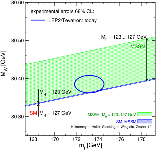
Figure 16: Prediction for $M_{W}$ in the MSSM and the SM (see text) as a function of $m_{t}$ in comparison with the present experimental results for $M_{W}$ and $m_{t}$ (updated from Ref. Heinemeyer:2006px , see Refs. PomssmRep ; MWlisa for more details).

As mentioned above, in order to restrict the number of free parameters in the MSSM one can resort to GUT based models. Most fits have been performed in the Constrained MSSM (CMSSM), in which the input scalar masses $m_{0}$, gaugino masses $m_{1/2}$ and soft trilinear parameters $A_{0}$ are each universal at the GUT scale, $M_{\rm GUT}\approx 2\times 10^{16}\,\,\mathrm{GeV}$, and in the Non-universal Higgs mass model (NUHM1), in which a common SUSY-breaking contribution to the Higgs masses is allowed to be non-universal (see Ref. newbenchmark for detailed definitions). The results for the fits of $M_{h}$ in the CMSSM and the NUHM1 are shown in Fig. 17 in the left and right plot, respectively mc8 . Also shown in Fig. 17 are as light shaded (green) band is the mass range corresponding to the newly discovered particle around $\sim 125\,\,\mathrm{GeV}$. One can see that the CMSSM is still compatible with $M_{h}\sim 125\,\,\mathrm{GeV}$, while the NUHM1 is in perfect agreement with this light ${\cal CP}$-even Higgs boson mass.

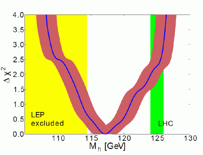
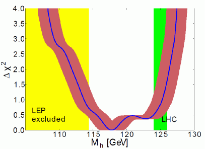
Figure 17: The $\Delta\chi^{2}$ functions for $M_{h}$ in the CMSSM (left) and the NUHM1 (right) mc8 , including the theoretical uncertainties (red bands). Also shown as light shaded (green) band is the mass range corresponding to the newly discovered particle around $\sim 125\,\,\mathrm{GeV}$.

Acknowledgments

I thank the organizers for their hospitality and for creating a very stimulating environment, in particular during the Whisky tasting.

References

- (1)
- (2) P. W. Higgs, Phys. Lett. 12 (1964) 132; Phys. Rev. Lett. 13 (1964) 508; Phys. Rev. 145 (1966) 1156; F. Englert and R. Brout, Phys. Rev. Lett. 13 (1964) 321; G. S. Guralnik, C. R. Hagen and T. W. B. Kibble, Phys. Rev. Lett. 13 (1964) 585.
- (3) G. Aad et al. [ATLAS Collaboration], Phys. Lett. B 716 (2012) 1 [arXiv:1207.7214 [hep-ex]].
- (4) S. Chatrchyan et al. [CMS Collaboration], Phys. Lett. B 716 (2012) 30 [arXiv:1207.7235 [hep-ex]].
- (5) CDF Collaboration, DØCollaboration, [arXiv:1207.0449 [hep-ex]].
- (6) S.L. Glashow, Nucl. Phys. B 22 (1961) 579; S. Weinberg, Phys. Rev. Lett. 19 (1967) 19; A. Salam, in: Proceedings of the 8th Nobel Symposium, Editor N. Svartholm, Stockholm, 1968.
- (7) H. Nilles, Phys. Rept. 110 (1984) 1; H. Haber and G. Kane, Phys. Rept. 117 (1985) 75; R. Barbieri, Riv. Nuovo Cim. 11 (1988) 1.
- (8) S. Heinemeyer, O. Stål and G. Weiglein, Phys. Lett. B 710 (2012) 201 [arXiv:1112.3026 [hep-ph]];
- (9) S. Weinberg, Phys. Rev. Lett. 37 (1976) 657; J. Gunion, H. Haber, G. Kane and S. Dawson, The Higgs Hunter’s Guide (Perseus Publishing, Cambridge, MA, 1990), and references therein.
- (10) P. Fayet, Nucl. Phys. B 90 (1975) 104; Phys. Lett. B 64 (1976) 159; Phys. Lett. B 69 (1977) 489; Phys. Lett. B 84 (1979) 416; H.P. Nilles, M. Srednicki and D. Wyler, Phys. Lett. B 120 (1983) 346; J.M. Frere, D.R. Jones and S. Raby, Nucl. Phys. B 222 (1983) 11; J.P. Derendinger and C.A. Savoy, Nucl. Phys. B 237 (1984) 307; J. Ellis, J. Gunion, H. Haber, L. Roszkowski and F. Zwirner, Phys. Rev. D 39 (1989) 844; M. Drees, Int. J. Mod. Phys. A 4 (1989) 3635; U. Ellwanger, C. Hugonie and A. M. Teixeira, Phys. Rept. 496 (2010) 1 [arXiv:0910.1785 [hep-ph]]; M. Maniatis, Int. J. Mod. Phys. A 25 (2010) 3505 [arXiv:0906.0777 [hep-ph]].
- (11) N. Arkani-Hamed, A. Cohen and H. Georgi, Phys. Lett. B 513 (2001) 232 [arXiv:hep-ph/0105239]; N. Arkani-Hamed, A. Cohen, T. Gregoire and J. Wacker, JHEP 0208 (2002) 020 [arXiv:hep-ph/0202089].
- (12) N. Arkani-Hamed, S. Dimopoulos and G. Dvali, Phys. Lett. B 429 (1998) 263 [arXiv:hep-ph/9803315]; Phys. Lett. B 436 (1998) 257 [arXiv:hep-ph/9804398]; I. Antoniadis, Phys. Lett. B 246 (1990) 377; J. Lykken, Phys. Rev. D 54 (1996) 3693 [arXiv:hep-th/9603133]; L. Randall and R. Sundrum, Phys. Rev. Lett. 83 (1999) 3370 [arXiv:hep-ph/9905221].
- (13) G. Weiglein et al. [LHC/ILC Study Group], Phys. Rept. 426 (2006) 47 [arXiv:hep-ph/0410364].
- (14) A. De Roeck et al., Eur. Phys. J. C 66 (2010) 525 [arXiv:0909.3240 [hep-ph]].
-
(15)
LHC2TSP Working Group 1 (EWSB) report, see:
https://indico.cern.ch/
contributionDisplay.py?contribId=131&confId=175067 . - (16) N. Cabibbo, L. Maiani, G. Parisi and R. Petronzio, Nucl. Phys. B 158 (1979) 295; R. Flores and M. Sher, Phys. Rev. D 27 (1983) 1679; M. Lindner, Z. Phys. C 31 (1986) 295; M. Sher, Phys. Rept. 179 (1989) 273; J. Casas, J. Espinosa and M. Quiros, Phys. Lett. 342 (1995) 171. [arXiv:hep-ph/9409458].
- (17) G. Altarelli and G. Isidori, Phys. Lett. B 337 (1994) 141; J. Espinosa and M. Quiros, Phys. Lett. 353 (1995) 257 [arXiv:hep-ph/9504241].
- (18) T. Hambye and K. Riesselmann, Phys. Rev. D 55 (1997) 7255 [arXiv:hep-ph/9610272].
- (19) See: https://twiki.cern.ch/twiki/bin/view/LHCPhysics/CrossSections .
- (20) S. Dittmaier et al. [LHC Higgs Cross Section Working Group Collaboration], arXiv:1101.0593 [hep-ph].
- (21) S. Dittmaier et al. [LHC Higgs Cross Section Working Group Collaboration], arXiv:1201.3084 [hep-ph].
- (22) A. Denner, S. Heinemeyer, I. Puljak, D. Rebuzzi and M. Spira, Eur. Phys. J. C 71 (2011) 1753 [arXiv:1107.5909 [hep-ph]].
- (23) ATLAS Collaboration, ATLAS-CONF-2012-170.
- (24) CMS Collaboration, CMS-PAS-HIG-12-045.
- (25) LHC Higgs Cross Section Working Group, A. David et al., arXiv:1209.0040 [hep-ph].
-
(26)
LEP Electroweak Working Group,
see: lepewwg.web.cern.ch/LEPEWWG/Welcome.html . - (27) Tevatron Electroweak Working Group, see: tevewwg.fnal.gov .
- (28) [The ALEPH, DELPHI, L3 and OPAL Collaborations, the LEP Electroweak Working Group], arXiv:1012.2367 [hep-ex]. see http://lepewwg.web.cern.ch/LEPEWWG/ .
- (29) A. Sirlin, Phys. Rev. D 22 (1980) 971; W. Marciano and A. Sirlin, Phys. Rev. D 22 (1980) 2695.
- (30) M. Veltman, Nucl. Phys. B 123 (1977) 89.
- (31) LEP Higgs working group, Phys. Lett. B 565 (2003) 61 [arXiv:hep-ex/0306033].
- (32) Tevatron Electroweak Working Group and CDF Collaboration and D0 Collaboration, arXiv:1107.5255 [hep-ex].
- (33) M. Grünewald, arXiv:0709.3744 [hep-ex]; arXiv:0710.2838 [hep-ex].
- (34) M. Grünewald, priv. communication.
- (35) M. Baak et al., Eur. Phys. J. C 72 (2012) 2205 [arXiv:1209.2716 [hep-ph]].
- (36) G. Montagna, O. Nicrosini, F. Piccinini and G. Passarino, Comput. Phys. Commun. 117 (1999) 278 [arXiv:hep-ph/9804211].
- (37) D. Bardin et al., Comput. Phys. Commun. 133 (2001) 229 [arXiv:hep-ph/9908433]; A. Arbuzov et al., Comput. Phys. Commun. 174 (2006) 728 [arXiv:hep-ph/0507146].
- (38) U. Baur, R. Clare, J. Erler, S. Heinemeyer, D. Wackeroth, G. Weiglein and D. Wood, arXiv:hep-ph/0111314.
- (39) J. Erler, S. Heinemeyer, W. Hollik, G. Weiglein and P. Zerwas, Phys. Lett. B 486 (2000) 125 [arXiv:hep-ph/0005024]; J. Erler and S. Heinemeyer, arXiv:hep-ph/0102083.
- (40) R. Hawkings and K. Mönig, EPJdirect C8 (1999) 1 [arXiv:hep-ex/9910022].
- (41) G. Wilson, LC-PHSM-2001-009, see: www.desy.de/lcnotes/notes.html.
- (42) A. Hoang et al., Eur. Phys. Jour. C 3 (2000) 1 [arXiv:hep-ph/0001286]; M. Martinez, R. Miquel, Eur. Phys. Jour. C 27 (2003) 49 [arXiv:hep-ph/0207315].
- (43) G. Aad et al. [The ATLAS Collaboration], arXiv:0901.0512.
- (44) G. Bayatian et al. [CMS Collaboration], J. Phys. G 34 (2007) 995.
- (45) S. Heinemeyer et al., arXiv:hep-ph/0511332.
- (46) S. Glashow and S. Weinberg, Phys. Rev. D 15 (1977) 1958.
-
(47)
B. Petersen, talk given at HCP2012, see:
http://kds.kek.jp/materialDisplay.py
?contribId=46&sessionId=20&materialId=slides&confId=9237; R. Gray, talk given at HCP2012, see: http://kds.kek.jp/materialDisplay.py
?contribId=48&sessionId=20&materialId=slides&confId=9237 . - (48) A. Djouadi, Phys. Rept. 459 (2008) 1 [arXiv:hep-ph/0503173].
- (49) J. Gunion, H. Haber, G. Kane and S. Dawson, The Higgs Hunter’s Guide, Addison-Wesley, 1990.
- (50) S. Heinemeyer, Int. J. Mod. Phys. A 21 (2006) 2659 [arXiv:hep-ph/0407244].
- (51) LEP Higgs working group, Eur. Phys. J. C 47 (2006) 547 [arXiv:hep-ex/0602042].
- (52) J. Ellis, G. Ridolfi and F. Zwirner, Phys. Lett. B 257 (1991) 83; Y. Okada, M. Yamaguchi and T. Yanagida, Prog. Theor. Phys. 85 (1991) 1; H. Haber and R. Hempfling, Phys. Rev. Lett. 66 (1991) 1815.
- (53) A. Brignole, Phys. Lett. B 281 (1992) 284.
- (54) P. Chankowski, S. Pokorski and J. Rosiek, Phys. Lett. B 286 (1992) 307; Nucl. Phys. B 423 (1994) 437, hep-ph/9303309.
- (55) A. Dabelstein, Nucl. Phys. B 456 (1995) 25, hep-ph/9503443; Z. Phys. C 67 (1995) 495, hep-ph/9409375.
- (56) R. Hempfling and A. Hoang, Phys. Lett. B 331 (1994) 99, hep-ph/9401219.
- (57) S. Heinemeyer, W. Hollik and G. Weiglein, Phys. Rev. D 58 (1998) 091701, hep-ph/9803277; Phys. Lett. B 440 (1998) 296, hep-ph/9807423.
- (58) S. Heinemeyer, W. Hollik and G. Weiglein, Eur. Phys. Jour. C 9 (1999) 343, hep-ph/9812472.
- (59) R. Zhang, Phys. Lett. B 447 (1999) 89, hep-ph/9808299; J. Espinosa and R. Zhang, JHEP 0003 (2000) 026, hep-ph/9912236.
- (60) G. Degrassi, P. Slavich and F. Zwirner, Nucl. Phys. B 611 (2001) 403, hep-ph/0105096.
- (61) J. Espinosa and R. Zhang, Nucl. Phys. B 586 (2000) 3, hep-ph/0003246.
- (62) A. Brignole, G. Degrassi, P. Slavich and F. Zwirner, Nucl. Phys. B 631 (2002) 195, hep-ph/0112177.
- (63) A. Brignole, G. Degrassi, P. Slavich and F. Zwirner, Nucl. Phys. B 643 (2002) 79, hep-ph/0206101.
- (64) S. Heinemeyer, W. Hollik, H. Rzehak and G. Weiglein, Eur. Phys. J. C 39 (2005) 465 [arXiv:hep-ph/0411114].
- (65) T. Banks, Nucl. Phys. B 303 (1988) 172; L. Hall, R. Rattazzi and U. Sarid, Phys. Rev. D 50 (1994) 7048, hep-ph/9306309; R. Hempfling, Phys. Rev. D 49 (1994) 6168; M. Carena, M. Olechowski, S. Pokorski and C. Wagner, Nucl. Phys. B 426 (1994) 269, hep-ph/9402253.
- (66) M. Carena, D. Garcia, U. Nierste and C. Wagner, Nucl. Phys. B 577 (2000) 577, hep-ph/9912516.
- (67) G. Degrassi, A. Dedes and P. Slavich, Nucl. Phys. B 672 (2003) 144, hep-ph/0305127.
- (68) S. Martin, Phys. Rev. D 65 (2002) 116003 [arXiv:hep-ph/0111209]; Phys. Rev. D 66 (2002) 096001 [arXiv:hep-ph/0206136]; Phys. Rev. D 67 (2003) 095012 [arXiv:hep-ph/0211366]; Phys. Rev. D 68 (2003) 075002 [arXiv:hep-ph/0307101]; Phys. Rev. D 70 (2004) 016005 [arXiv:hep-ph/0312092]; Phys. Rev. D 71 (2005) 016012 [arXiv:hep-ph/0405022]; Phys. Rev. D 71 (2005) 116004 [arXiv:hep-ph/0502168]; Phys. Rev. D 75 (2007) 055005 [arXiv:hep-ph/0701051]; S. Martin and D. Robertson, Comput. Phys. Commun. 174 (2006) 133 [arXiv:hep-ph/0501132].
- (69) R. Harlander, P. Kant, L. Mihaila and M. Steinhauser, Phys. Rev. Lett. 100 (2008) 191602 [Phys. Rev. Lett. 101 (2008) 039901] [arXiv:0803.0672 [hep-ph]]; JHEP 1008 (2010) 104 [arXiv:1005.5709 [hep-ph]].
- (70) G. Degrassi, S. Heinemeyer, W. Hollik, P. Slavich and G. Weiglein, Eur. Phys. J. C 28 (2003) 133 [arXiv:hep-ph/0212020].
- (71) S. Heinemeyer, W. Hollik and G. Weiglein, Phys. Rept. 425 (2006) 265 [arXiv:hep-ph/0412214].
- (72) S. Heinemeyer, W. Hollik and G. Weiglein, Comput. Phys. Commun. 124 (2000) 76 [arXiv:hep-ph/9812320]; T. Hahn, S. Heinemeyer, W. Hollik, H. Rzehak and G. Weiglein, Comput. Phys. Commun. 180 (2009) 1426, see: www.feynhiggs.de .
- (73) M. Frank, T. Hahn, S. Heinemeyer, W. Hollik, H. Rzehak and G. Weiglein, JHEP 0702 (2007) 047 [arXiv:hep-ph/0611326].
- (74) M. Diaz and H. Haber, Phys. Rev. D 45 (1992) 4246.
- (75) M. Frank, PhD thesis, university of Karlsruhe, 2002.
- (76) M. Carena, S. Heinemeyer, C. Wagner and G. Weiglein, Eur. Phys. J. C 26 (2003) 601 [arXiv:hep-ph/0202167].
- (77) T. Hahn, S. Heinemeyer, F. Maltoni, G. Weiglein and S. Willenbrock, arXiv:hep-ph/0607308.
- (78) R. Harlander, S. Liebler and H. Mantler, arXiv:1212.3249 [hep-ph].
- (79) G. Degrassi and P. Slavich, Nucl. Phys. B 805 (2008) 267 [arXiv:0806.1495 [hep-ph]]; G. Degrassi, S. Di Vita and P. Slavich, JHEP 1108 (2011) 128 [arXiv:1107.0914 [hep-ph]]; Eur. Phys. J. C 72 (2012) 2032 [arXiv:1204.1016 [hep-ph]]; R. Harlander, H. Mantler, S. Marzani and K. Ozeren, Eur. Phys. J. C 66 (2010) 359 [arXiv:0912.2104 [hep-ph]]; R. Harlander, F. Hofmann and H. Mantler, JHEP 1102 (2011) 055 [arXiv:1012.3361 [hep-ph]].
- (80) M. Carena, S. Heinemeyer, C. Wagner and G. Weiglein, Eur. Phys. J. C 45 (2006) 797 [arXiv:hep-ph/0511023].
- (81) CMS Collaboration, CMS-PAS-HIG-12-050.
- (82) F. Gianotti for the ATLAS collaboration and G. Tonelli for the CMS collaboration, see: indico.cern.ch/conferenceDisplay.py?confId=164890 .
- (83) R. Benbrik, M. Gomez Bock, S. Heinemeyer, O. Stål, G. Weiglein and L. Zeune, Eur. Phys. J. C 72 (2012) 2171 [arXiv:1207.1096 [hep-ph]].
- (84) P. Bechtle, S. Heinemeyer, O. Stal, T. Stefaniak, G. Weiglein and L. Zeune, arXiv:1211.1955 [hep-ph].
- (85) P. Bechtle, O. Brein, S. Heinemeyer, G. Weiglein and K. E. Williams, Comput. Phys. Commun. 181 (2010) 138 [arXiv:0811.4169 [hep-ph]]; Comput. Phys. Commun. 182 (2011) 2605 [arXiv:1102.1898 [hep-ph]]; P. Bechtle, O. Brein, S. Heinemeyer, O. Stål, T. Stefaniak, G. Weiglein and K. Williams, arXiv:1301.2345 [hep-ph].
- (86) S. Heinemeyer, W. Hollik, D. Stockinger, A. M. Weber and G. Weiglein, JHEP 0608 (2006) 052 [arXiv:hep-ph/0604147].
- (87) S. Heinemeyer, G. Weiglein and L. Zeune, DESY 13–015, in preparation.
- (88) S. AbdusSalam, et al., Eur. Phys. J. C 71 (2011) 1835 [arXiv:1109.3859 [hep-ph]].
- (89) O. Buchmueller et al., Eur. Phys. J. C 72 (2012) 2243 [arXiv:1207.7315 [hep-ph]].