Anisotropic branes

Souvik Banerjee ^†, Samrat Bhowmick ^†, Sudipta Mukherji ^†
Institute of Physics
Bhubaneswar -751 005, India

Abstract

We present a class of anisotropic brane configurations which shows BKL oscillations near their cosmological singularities. Near horizon limits of these solutions represent Kasner space embedded in AdS background. Dynamical probe branes in these geometries inherit anisotropies from the background. Amusingly, for a probe M5 brane, we find that there exists a parameter region where three of its world-volume directions expand while the rest contract.

${}^{\dagger}~{}~{}$ e-mail address: souvik, samrat, mukherji@iopb.res.in

Introduction

AdS/CFT correspondence proposes an equivalence between the string theory in AdS space and a conformal field theory on its boundary. One of the remarkable features of this correspondence is the fact that it relates a strongly coupled theory with a weakly coupled one. Consequently, it provides us with a way to tame the non-perturbative region of one by performing computations on its dual. Due to strong gravitational fluctuations, physics around cosmological singularities is dominated by non-perturbative effects and one hopes that the AdS/CFT correspondence would shed some light into it. Indeed, in recent years, we have witnessed several important investigations where attempts were made to find the signatures of these singularities in their gauge theory duals. Expectation is that the dual theory evolution might be able to provide a sensible quantum description of these singularities. Successes have been varied, please see the references [1] - [5].

Inspired by this line of developments, in this letter, we search for D brane solutions in ten dimensional type IIB theory where the world volume metric expands anisotropically and show instabilities within their supergravity descriptions. We find that appropriately tuning the five form field strength, it is possible to construct a D3 brane with four dimensional Kasner like world volume. Along with a time-like singularity at $r=0$, the metric shows an additional cosmological singularity at $t=0$. Perturbation around $t=0$ generates an analogue of Belinskii-Lifshitz-Khalatnikov (BKL) oscillations. The near horizon geometry of this brane reduces to that of a Kasner-universe in AdS space plus a five sphere along with an appropriate five form field strength. We further probe the geometry by a dynamical D3 brane whose world-volume inherits anisotropic expansion/contraction along with a BKL like oscillation. Similar solutions can be constructed even within eleven dimensional supergravity. As an illustrative example, we discuss the case of M5 brane. The near horizon geometry is now a six dimensional Kasner space. A dynamical probe M5 brane in this space-time again acquires an anisotropic expansion in some directions and contraction along some. Amusingly, we find that it is possible to tune parameters in such a manner that three directions expand and the rest contract. Close to the cosmological singularities supergravity descriptions of all these solutions are expected to break down. We hope that the gauge theory description would shed some light on the physics near the singularities.

D3 brane with anisotropic time-dependent world volume

Besides the static D branes of odd space dimensions, the IIB string theory admits time dependent branes. Consider, for example, the case of D3 brane. The equations of motion following from the relevant part of standard IIB supergravity action

$$S_{IIB}=-\frac{1}{16\pi G_{10}}\int d^{10}x\sqrt{-g}\left(R-\frac{1}{2}\partial^{\mu}\phi\partial_{\mu}\phi-\frac{1}{2\times 5!}F_{5}^{2}\right)\;.$$ (1)

has the following forms:

$$R^{\mu}_{\nu}=\frac{1}{2}\partial^{\mu}\phi\partial_{\nu}\phi+\frac{1}{2\times 5!}(5F^{\mu\xi_{2}...\xi_{5}}F_{\nu\xi_{2}...\xi_{5}}-\frac{1}{2}\delta^{\mu}_{\nu}F_{5}^{2}),$$

$$\partial_{\mu}({\sqrt{g}}F^{\mu\xi_{2}...\xi_{5}})=0,$$

$$\nabla^{2}\phi=0.$$ (2)

These equations are solved by

$$ds^{2}=\Big{(}1+\frac{l^{4}}{r^{4}}\Big{)}^{-\frac{1}{2}}\Big{[}-dt^{2}+t^{2\alpha}dx^{2}+t^{2\beta}dy^{2}+t^{2\gamma}dz^{2}\Big{]}+\Big{(}1+\frac{l^{4}}{r^{4}}\Big{)}^{\frac{1}{2}}\Big{[}dr^{2}+r^{2}d\Omega_{5}^{2}\Big{]},$$

$$F_{txyzr}=\frac{4l^{4}t^{\alpha+\beta+\gamma}r^{3}}{(l^{4}+r^{4})^{2}},$$

$$\phi=0,$$ (3)

provided

$$\alpha+\beta+\gamma=1~{}~{}~{}{\rm and}~{}\alpha^{2}+\beta^{2}+\gamma^{2}=1.$$ (4)

The numbers $\alpha,\beta,\gamma$ can be organized in an increasing order $\alpha<\beta<\gamma$ and they vary in the range

$$-\frac{1}{3}\leq\alpha\leq 0,~{}~{}0\leq\beta\leq\frac{2}{3},~{}~{}{\rm and}~{}\frac{2}{3}\leq\gamma\leq 1.$$ (5)

These numbers can also be parametrized as

$$\alpha(u)=\frac{-u}{1+u+u^{2}},~{}~{}\beta(u)=\frac{1+u}{1+u+u^{2}},~{}~{}\gamma(u)=\frac{u+u^{2}}{1+u+u^{2}},$$ (6)

where the Lifshitz-Khalatnikov parameter $u\geq 1$. Further, values $u<1$ lead to the same range as

$$\alpha(\frac{1}{u})=\alpha(u),~{}~{}\beta(\frac{1}{u})=\beta(u),~{}~{}\gamma(\frac{1}{u})=\gamma(u).$$ (7)

The five form charge can be calculated by integrating $*F_{5}$ over the transverse space and it turns out to be time independent.

In our convention, the extremal D3 brane is represented by $\alpha=\beta=\gamma=0$ and is not continuously connected to the above solution. Unlike extremal $D3$ brane, this solution breaks all the supersymmetries of IIB theory due to its explicit time dependence. The Kretschmann scalar for the metric is given by

$$R_{\mu\nu\rho\sigma}R^{\mu\nu\rho\sigma}=\frac{16(-\alpha^{2}(l^{4}+r^{4})^{6}+\alpha^{3}(l^{4}+r^{4})^{6}-5l^{8}r^{4}(l^{8}+12r^{8})t^{4})}{r^{4}(l^{4}+r^{4})^{5}t^{4}}.$$ (8)

In writing the above equation, we have used the condition (4). It has a time-like singularity at $r=0$ at any finite time. It, further, has a cosmological singularity at $t=0$.

In the large $r$ limit, equations in (3) reduce to a four dimensional Kasner solution plus a flat six-dimensional part. Within the Bianchi classification of homogeneous spaces, the Kasner metric corresponds to choosing all three of the structure constants to be zero. A generic perturbation near the singularity breaks these constraints generating Belinskii-Lifshitz-Khalatnikov (BKL) oscillations [6]. To briefly illustrate the BKL oscillation, appropriately generalized to our context, we replace the world volume metric on the brane by type IX homogeneous space.

To this end, let us consider the brane configuration of the form

$$ds^{2}=\Big{(}1+\frac{l^{4}}{r^{4}}\Big{)}^{-\frac{1}{2}}\big{[}-dt^{2} + (a(t)^{2}l_{i}l_{j}+b(t)^{2}m_{i}m_{j}+c(t)^{2}n_{i}n_{j})dx^{i}dx^{j}\Big{]}$$ (9)

$$+ \Big{(}1+\frac{l^{4}}{r^{4}}\Big{)}^{\frac{1}{2}}\Big{[}dr^{2}+r^{2}d\Omega_{5}^{2}\Big{]}\;.$$

with the anti-symmetric five form field and the scalar

$$F_{txyzr}=\frac{4r^{3}l^{4}a(t)b(t)c(t)\sin(x)}{\left(r^{4}+l^{4}\right)^{2}}\;,$$ (11)

$$\phi=0\;.$$

Here $l_{i},m_{i},n_{i}$ are frame vectors. For IX metric, all the three structure constants are 1 and the simplest choice for the frame vectors is

$$l_{i}=({\rm sin}x,-{\rm cos}z~{}{\rm sin}x,0),~{}m_{i}=({\rm cos}x,{\rm sin}z~{}{\rm sin}x,0),~{}n_{i}=(0,{\rm cos}x,1).$$ (12)

The coordinates run through values in the ranges $0\leq x\leq\pi$, $0\leq y\leq 2\pi$, $0\leq z\leq 4\pi$. The above configuration (9 - 11) is a solution provided they satisfy IIB equations of motion (2). This requirement leads to the following differential equations for $a,b$ and $c$.

$$\frac{(a_{t}bc)_{t}}{abc}=\frac{1}{2a^{2}b^{2}c^{2}}\big{[}(b^{2}-c^{2})^{2}-a^{4}\big{]}\;,$$

$$\frac{(ab_{t}c)_{t}}{abc}=\frac{1}{2a^{2}b^{2}c^{2}}\big{[}(c^{2}-a^{2})^{2}-b^{4}\big{]}\;,$$

$$\frac{(abc_{t})_{t}}{abc}=\frac{1}{2a^{2}b^{2}c^{2}}\big{[}(a^{2}-b^{2})^{2}-c^{4}\big{]}\;,$$

$$\frac{a_{tt}}{a}+\frac{b_{tt}}{b}+\frac{c_{tt}}{c}=0\;,$$ (13)

where the subscript indicates derivative with respect to $t$. These are exactly the equations responsible for generating standard BKL oscillations. Consequently, the brane world-volume metric will oscillate with negative powers of $t$ oscillating from one direction to another. In the next paragraph, for the sake of completeness, we give a brief analysis of this oscillation.

To proceed, first we notice that if all the expressions on the right hand side of (13) are small in some region, the system will have a Kasner-like regime with

$$a\sim t^{\alpha},b\sim t^{\beta},~{}c\sim t^{\gamma},$$ (14)

where $\alpha,\beta,\gamma$ satisfy constraint as in (4). However, now since $\alpha$ is negative, close to $t=0$, $a^{4}$ term in the right hand sides of (13) will start dominating. It is useful to write these equation in terms of new variables defined as

$$a=e^{p},~{}b=e^{q},~{}c=e^{s},~{}e^{p+q+s}d\tau=dt.$$ (15)

In the vicinity of $t=0$, (13) reduces to

$$p_{\tau\tau}=-\frac{1}{4}e^{4p},q_{\tau\tau}=s_{\tau\tau}=\frac{1}{2}e^{4p},$$ (16)

where the subscripts $\tau$ indicates derivative with respect to $\tau$. The solution of these equations should describe the evolution of world-volume metric from the initial state of Kasner metric. In terms of the new variables, this is equivalent to

$$p_{\tau}=\alpha,~{}q_{\tau}=\beta,~{}s_{\tau}=\gamma.$$ (17)

Note that the first equation in (16) can be interpreted as a particle moving in the presence of an exponential wall-like potential. Due to the reflection from this barrier, particle will move with $p_{\tau}=-\alpha$. However we see from (16) that $p_{\tau}+q_{\tau}$ and $p_{\tau}+s_{\tau}$ are constants. So we get

$$q_{\tau}=\beta+2\alpha,~{}s_{\tau}=\gamma+2\alpha.$$ (18)

These lead to

$$e^{p}=e^{-\alpha\tau},~{}e^{q}=e^{(\beta+2\alpha)\tau},~{}e^{\tau}=e^{(\gamma+2\alpha)\tau}~{}{\rm and}~{}~{}t\sim e^{(1+2\alpha)\tau}.$$ (19)

In terms of the original variables, we can re-write the above as

$$a=t^{\frac{|\alpha|}{1-2|\alpha|}},~{}b=t^{\frac{\beta-2|\alpha|}{1-2|\alpha|}},~{}c=t^{\frac{\gamma-2|\alpha|}{1-2|\alpha|}}.$$ (20)

Therefore the action of the perturbation results oscillations between one Kasner regime to another with negative power shifting from $a$ to $b$ to $c$, inducing BKL oscillations on the world-volume of the D3 brane. We should however note that near the curvature singularity, string action receives higher derivative gravitational corrections. Consequently, the nature of the singularity and behaviour of its perturbation may get substantially modified. Solutions may also get modified when one introduces other matter fields into the theory. If they are represented by a perfect fluids on the world-volume, with pressure and energy density related as $p=\omega\rho$, it can be argued that for $\omega<1$, BKL oscillations still persist. However, situation changes drastically for $\omega=1$, namely for the stiff-matter (a massless scalar field for example). A general discussion on these issues can be found in [8, 10]. Indeed it is easy to check that in our previous solution, one can introduce a dilaton with a profile

$$\phi=\lambda\,\log t.$$ (21)

The metric and the form field remains same as before. However, the exponents now satisfy new constraint relations : $\alpha+\beta+\gamma=1,~{}~{}\alpha^{2}+\beta^{2}+\gamma^{2}=1-\lambda^{2}$. The changes in these relations allow BKL oscillation for a finite time and the system finally reaches an attractor.

We now proceed to study the metric in the near horizon limit $r\rightarrow 0$. In this limit, the metric reduces to

$$ds^{2}=-\frac{r^{2}}{l^{2}}dt^{2}+\frac{l^{2}}{r^{2}}dr^{2}+r^{2}(t^{2\alpha}dx^{2}+t^{2\beta}dy^{2}+t^{2\gamma}dz^{2})+l^{2}d\Omega_{5}^{2},$$ (22)

with

$$F_{txyzr}=\frac{4tr^{3}}{l^{4}},~{}~{}{\rm giving~{}potential}~{}C_{txyz}=\frac{tr^{4}}{l^{4}}.$$ (23)

The Kretschmann scalar is,

$$R_{\mu\nu\rho\sigma}R^{\mu\nu\rho\sigma}=\frac{16\alpha^{2}(\alpha-1)l^{4}}{r^{4}t^{4}}-\frac{80}{l^{4}}.$$ (24)

We call it a Kasner-AdS space. This Kasner-AdS solution separately satisfies five dimensional Einstein equation in the presence of a negative cosmological constant and was found in [11] in the context of brane-cosmology.

Probing with a D3 brane

In this section, we will probe the geometry (3) with a D3 brane. Distance of the probe brane from the source now behaves as a scalar whose explicit time dependence can be determined via a dynamical equation. We take the world-volume directions of the D3 brane as $\xi=(t,x,y,z)$. The world-volume action of the D3 brane in background geometry, (3) takes the form :

$$S=T\int d^{4}\xi\sqrt{-det\ G_{\alpha\beta}}+T\int d^{4}\xi\,\hat{C_{4}},$$ (25)

Here $G_{\alpha\beta}$ is the induced metric on the world-volume and $\hat{C_{4}}$ is the pull-back of the background $4$-form potential. $T$ is the brane tension. We turn off all other fields on the brane.
The Lagrangian can be cast in the form :

$$L=\sqrt{A(t,r)\ -\ B(t,r)\ \dot{r}^{2}\ }-C(r),$$ (26)

where,

$$A(t,r) = t^{2}\ \left(1+\frac{l^{4}}{r^{4}}\right)^{-2}$$

$$B(t,r) = t^{2}\ \left(1+\frac{l^{4}}{r^{4}}\right)^{-1}$$

$$C(r) = -\frac{t\ {l^{4}}}{{l^{4}}+{r^{4}}}$$

The equation of motion for $r(t)$ is the Euler-Lagrange equation derived from (Probing with a D3 brane) :

$$r^{4}\big{(}l^{4}+r^{4}\big{)}^{2}[t\ddot{r}+\dot{r}]-(l^{4}+r^{4})^{3}\dot{r}^{3}-2tl^{4}r^{3}\left[3(l^{4}+r^{4})\dot{r}^{2}-2r^{4}\right]$$

$$-4tl^{4}r\left[r^{4}-\left(l^{4}+r^{4}\right)\dot{r}^{2}\right]^{\frac{3}{2}}=0$$ (28)

Here dot represents derivative with respect to $t$. Once this equation is solved with appropriate boundary conditions, the metric on the probe brane is uniquely determined. We will carry out this computation in this section. However, owing to the explicit time dependence in the background geometry, we find that the dynamical equation can not be solved analytically. Fortunately, it is not hard to find numerical solution and a typical behaviour is shown in the figure 1.

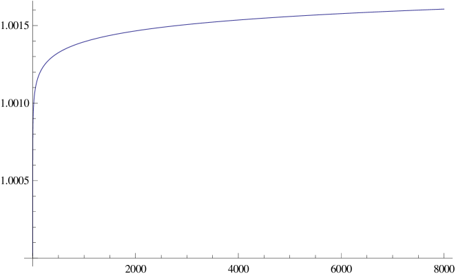
Figure 1: Plot of $r$ as a function of time, $t$.

The functions that govern the anisotropic expansions in three spatial directions are $t^{\alpha}\ f(r)$, $t^{\beta}\ f(r)$, $t^{\gamma}\ f(r)$, where

$$f(r)=\left(1+\frac{l^{4}}{r^{4}}\right)^{-\frac{1}{4}}.$$ (29)

In order that the near horizon geometry is an $AdS$, as mentioned earlier, $\alpha$,$\beta$,$\gamma$ must satisfy the constraint : $\alpha^{2}+\beta^{2}+\gamma^{2}=\alpha+\beta+\gamma=1$. This means, once we specify one of the three, say, $\alpha$, the other two are automatically fixed :

$$\beta = \frac{1}{2}\left(1-\alpha+\sqrt{-3\alpha^{2}+2\alpha+1}\right)$$

$$\gamma = \frac{1}{2}\left(1-\alpha-\sqrt{-3\alpha^{2}+2\alpha+1}\right)$$ (30)

Ideally, in cosmology, one defines cosmological time, $\eta$ with which the metric on the probe brane takes the form :

$$dS_{brane}^{2}=-d\eta^{2}+\left(1+\frac{l^{4}}{r^{4}(\eta)}\right)^{-\frac{1}{2}}(t^{2\alpha}(\eta)dx^{2}+t^{2\beta}(\eta)dy^{2}+t^{2\gamma}(\eta)dz^{2}).$$ (31)

with

$$\frac{d\eta}{dt}=\sqrt{\left(1+\frac{l^{4}}{r^{4}}\right)^{-\frac{1}{2}}-\left(1+\frac{l^{4}}{r^{4}}\right)^{\frac{1}{2}}\left(\frac{dr(t)}{dt}\right)^{2}}.$$ (32)

The behaviour of time, $t$ as a function of $\eta$ is depicted in figure 2.

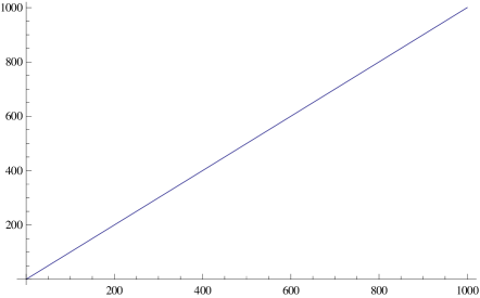
Figure 2: Plot of $t$ as a function of $\eta$.

At this, we plot the functions $t^{\alpha}\ f(r)$, $t^{\beta}\ f(r)$, $t^{\gamma}\ f(r)$ as functions of $\eta$ parametrically. Here $f(r)$ is defined through (29). One can tune the values of $\alpha$, $\beta$, $\gamma$ consistent with the Kasner constraints so that one of them goes down to zero (decelerating) while two of them go up (accelerating) with cosmic time and vice versa. One such plot is given in figure 3.

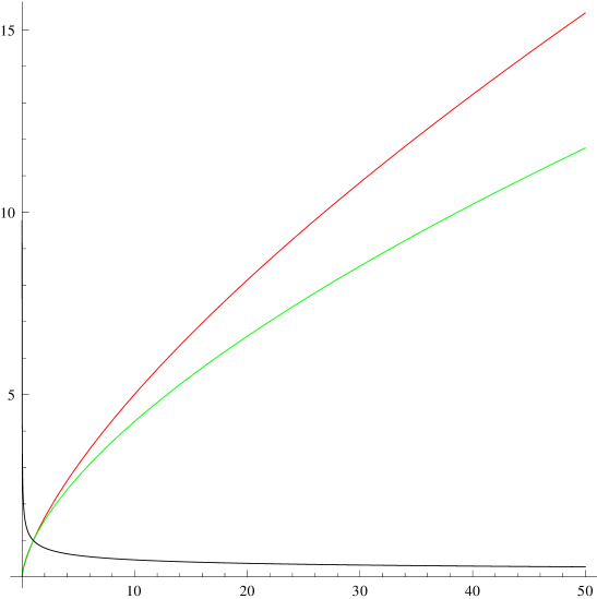
Figure 3: The functions, $f_{1}=t^{\alpha}(\eta)\ f(r)$, $f_{2}=t^{\beta}(\eta)\ f(r)$, $f_{3}=t^{\gamma}(\eta)\ f(r)$, with $f(r)$ given in (29) are plotted as functions of $\eta$. $\alpha$, $\beta$ and $\gamma$ are 0.7, .632, -0.332 respectively The plot of $f_{1}$ is in red, and that of $f_{2}$ and $f_{3}$ are in green and black respectively.

The M5 Brane

Our previous discussion can easily be extended to eleven dimensions. Here we discuss the case of a M5 brane. We start with $d=11$ supergravity action

$$S_{11d}=-\frac{1}{2\ \kappa_{11}^{2}}\int d^{11}x\sqrt{-g}\left(R-\frac{1}{48}\ F_{4}^{2}\right)\;,$$ (33)

which is a generic action for the bosonic part of $d=11$ supergravity so long as we concentrate on static, flat translationally invariant p-brane solutions.

The equations of motion arising from (33) admits a solution of the form :

$$ds^{2} = \left(1+\frac{l^{3}}{r^{3}}\right)^{-\frac{1}{3}}\left[-dt^{2}+t^{2\alpha_{1}^{2}}dx_{1}^{2}+t^{2\alpha_{2}^{2}}dx_{2}^{2}+t^{2\alpha_{3}^{2}}dx_{3}^{2}+t^{2\alpha_{4}^{2}}dx_{4}^{2}+t^{2\alpha_{5}^{2}}dx_{5}^{2}\right]$$ (34)

$$+ \left(1+\frac{l^{3}}{r^{3}}\right)^{\frac{2}{3}}\left[dr^{2}+r^{2}d\Omega_{4}^{2}\right],$$

along with

$$F_{tx_{1}x_{2}x_{3}x_{4}x_{5}r}=\frac{3\ l^{3}\ t\ r^{2}}{(l^{3}+r^{3})^{2}}$$ (35)

provided $\alpha_{1}+\alpha_{2}+\alpha_{3}+\alpha_{4}+\alpha_{5}=1$ and $\alpha_{1}^{2}+\alpha_{2}^{2}+\alpha_{3}^{2}+\alpha_{4}^{2}+\alpha_{5}^{2}=1$.

In the near horizon limit, i.e. $r\rightarrow 0$, the metric and the non-zero component of the form field reduce to the forms :

$$ds^{2} = \frac{r}{l}\left[-dt^{2}+t^{2\alpha_{1}^{2}}dx_{1}^{2}+t^{2\alpha_{2}^{2}}dx_{2}^{2}+t^{2\alpha_{3}^{2}}dx_{3}^{2}+t^{2\alpha_{4}^{2}}dx_{4}^{2}+t^{2\alpha_{5}^{2}}dx_{5}^{2}\right]$$

$$+ \frac{l^{2}}{r^{2}}\left[dr^{2}+r^{2}d\Omega_{4}^{2}\right],$$

$$F_{tx_{1}x_{2}x_{3}x_{4}x_{5}r} = \frac{3\ t\ r^{2}}{l^{3}},$$ (36)

and hence the potential is given by $C_{tx_{1}x_{2}x_{3}x_{4}x_{5}}=\frac{t\ r^{3}}{l^{3}}$.

We now make the following change of coordinates :

$$w^{2}=\frac{r}{l^{3}}.$$ (37)

With this, the metric in (The M5 Brane) takes the form :

$$ds^{2}=\frac{w^{2}}{4l^{2}}\left(-d\bar{t}^{2}+\bar{t}^{2\alpha_{1}^{2}}d\bar{x}_{1}^{2}+\bar{t}^{2\alpha_{2}^{2}}d\bar{x}_{2}^{2}+\bar{t}^{2\alpha_{3}^{2}}d\bar{x}_{3}^{2}+\bar{t}^{2\alpha_{4}^{2}}d\bar{x}_{4}^{2}+\bar{t}^{2\alpha_{5}^{2}}d\bar{x}_{5}^{2}\right)+4\ l^{2}\frac{dw^{2}}{w^{2}}+l^{2}d\Omega_{4}^{2},$$ (38)

where $\bar{x}_{i}$ and $\bar{t}$ are suitably scaled versions of the coordinates, ${x}_{i}$ and ${t}$ respectively. It is worth mentioning in this regard that the scaling of the coordinates will not be the same because of the presence of different powers of $t$ in front of $dx_{i}^{2}$. This is a consequence of anisotropy.

Following our nomenclature, (38) is a metric of seven dimensional Kasner–Ads space plus a four sphere. For $\alpha_{i}=0$ for $i=1,...,5$, this reduces to our known $AdS_{7}(2L)\times S^{4}(L)$ solution.

Probing with a M5 brane

In the same spirit as we considered the case of probe D3 brane, we now consider a probe M5 brane in the background (34) and (35).

In PST formalism [12], the world-volume action of M5 brane is given in terms of a gauge invariant $3$-form field strength, ${\cal H}^{(3)}=d{\cal A}^{(2)}+{\cal C}^{(3)}$, where ${\cal A}^{(2)}$ is world-volume $2$-form and ${\cal C}^{(3)}$, target space $3$-form. The world volume action in this formalism is written as :

$$S_{M5}=T_{M5}\int d^{6}\xi\left[{\cal L}_{DBI}+{\cal L}_{KE}+{\cal L}_{WZ}\right],$$ (39)

where

$${\cal L}_{DBI} = \sqrt{-det\left(G_{ij}+{\tilde{\cal H}}_{ij}\right)}\quad{\text{is the Dirac-Born- Infeld Lagrangian,}}$$

$${\cal L}_{KE} = \frac{1}{24\left(\partial a\right)^{2}}\epsilon^{ijklmn}{\cal H}_{lmn}{\cal H}_{jkp}G^{pq}\partial_{i}a\partial_{q}a\quad{\text{is the kinetic piece for the $3$-form,}}$$

$${\cal L}_{WZ} = \frac{1}{6!}\epsilon^{ijklmn}\left[{\cal C}^{(6)}_{ijklmn}+10\ {\cal H}_{ijk}\ {\cal C}^{(3)}_{lmn}\right]{\text{is the Wess-Zumino term.}}$$

Here $S_{\alpha\beta}$ is the induced metric on the world-volume, ${\cal C}^{(3)}$ and ${\cal C}^{(6)}$ are the pull-backs of the $3$-form and $6$-form background potentials respectively. ${\tilde{\cal H}}$ is defined as

$${\tilde{\cal H}}^{ij}=\frac{1}{3!\sqrt{-detG}\ \sqrt{-(\partial a)^{2}}}\epsilon^{ijklmn}\partial_{k}a\ {\cal H}_{lmn}.$$ (41)

“$a$” is an auxiliary scalar field introduced in PST formalism to maintain manifest covariance.

If we now take the world-volume directions of the M5 brane as $\xi=(t,x_{1},x_{2},x_{3},x_{4},x_{5})$, it can be explicitly checked that, in this “static gauge”, there will be no component of ${\cal C}^{(3)}$ in world-volume directions. We further simplify the system by turning off the world-volume $2$-form, ${\cal A}^{(2)}$. With all these taken into account, the full Lagrangian takes the simple form :

$$L=\sqrt{A(t,r)\ -\ B(t,r)\ \dot{r}^{2}\ }-C(r),$$ (42)

where,

$$A(t,r) = t^{2}\ \left(1+\frac{l^{3}}{r^{3}}\right)^{-2}$$

$$B(t,r) = t^{2}\ \left(1+\frac{l^{3}}{r^{3}}\right)^{-1}$$

$$C(r) = -\frac{t\ {l^{3}}}{{l^{3}}+{r^{3}}}\,.$$

Here dot represents derivative with respect to $t$. The Euler Lagrange equation for $r(t)$ is :

$$2r^{4}\left(l^{3}+r^{3}\right)^{2}\left[t\ddot{r}+\dot{r}\right]-2r\left(l^{3}+r^{3}\right)^{3}\dot{r}^{3}-3tl^{3}r^{3}\left[3\left(l^{3}+r^{3}\right)\dot{r}^{2}-2r^{3}\right]$$

$$-6tl^{3}r^{\frac{3}{2}}\left[r^{3}-(l^{3}+r^{3})\dot{r}^{2}\right]^{\frac{3}{2}}=0\;.$$ (44)

In order to draw a cosmological interpretation of the solutions we obtain from (Probing with a M5 brane), as usual, we go to the “cosmic time” coordinate, $\eta$, in which the metric on the brane assumes a form :

$$ds_{{\it brane}}^{2}=-d{\eta(t)}^{2}+\left(1+\frac{l^{3}}{r^{3}(\eta)}\right)^{-\frac{1}{3}}\left(\sum_{i=1}^{5}{t}^{2\alpha_{i}}(\eta)d{x}_{i}^{2}\right)\,,$$ (45)

with

$$\frac{d\eta}{dt}=\sqrt{\left(1+\frac{l^{3}}{r^{3}}\right)^{-\frac{1}{3}}-\left(1+\frac{l^{3}}{r^{3}}\right)^{\frac{2}{3}}\left(\frac{dr(t)}{dt}\right)^{2}}.$$ (46)

The functions that govern the expansion of the universe in the spatial world-volume directions of the brane are in this case $t^{\alpha_{i}}\ f(r)$, where

$$f(r)=\left(1+\frac{l^{3}}{r^{3}}\right)^{-\frac{1}{6}}\;.$$ (47)

We can choose $\alpha_{i}$’s so that three of them are the same and mimics isotropic expansion in three directions. The other two are anisotropic. Such a situation can be parametrized as :

$$\alpha_{1} = \alpha_{2}=\alpha_{3}=p$$

$$\alpha_{4} = \frac{1}{2}\left(\sqrt{-15p^{2}+6p+1}-3p+1\right)$$

$$\alpha_{5} = \frac{1}{2}\left(-\sqrt{-15p^{2}+6p+1}-3p+1\right)\,.$$ (48)

Interestingly there exists a narrow window of parametric value for $p$, in which $\alpha_{i}$ for $i=1,2,3$ are positive and $\alpha_{4}$ and $\alpha_{5}$ are negative. An illustrative plot is shown in figure 4 for a particular value of $p$.

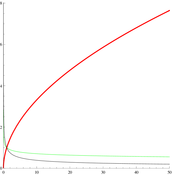
Figure 4: The functions, $t^{\alpha_{i}}(\eta)\ f(r)$, for $i=1,2,\cdots,5$ are plotted as functions of $\eta$ for $p=0.52$. This corresponding values for $\alpha_{i}$’s are : $\alpha_{1}=\alpha_{2}=\alpha_{3}=0.52$ , $\alpha_{4}=-0.15$ and $\alpha_{5}=-0.41$. The isotropic expansion corresponding to $\alpha_{1}$, $\alpha_{2}$, $\alpha_{3}$ is plotted in red. The contraction corresponding to $\alpha_{4}$, $\alpha_{5}$ are plotted in green and black respectively.

To conclude, we have presented a class of brane configurations which shows BKL oscillations near their cosmological singularities. It will be worthwhile to look for the signatures of these oscillations in their dual descriptions. We hope to report on this in the near future.

References

- [1] T. Hertog and G. T. Horowitz, JHEP 0504, 005 (2005) [hep-th/0503071].
- [2] B. Craps, T. Hertog and N. Turok, Phys. Rev. D 86, 043513 (2012) [arXiv:0712.4180 [hep-th]].
- [3] A. Awad, S. R. Das, S. Nampuri, K. Narayan and S. P. Trivedi, Phys. Rev. D 79, 046004 (2009) [arXiv:0807.1517 [hep-th]].
- [4] G. Horowitz, A. Lawrence and E. Silverstein, JHEP 0907, 057 (2009) [arXiv:0904.3922 [hep-th]].
- [5] A. Awad, S. R. Das, A. Ghosh, J. -H. Oh and S. P. Trivedi, Phys. Rev. D 80, 126011 (2009) [arXiv:0906.3275 [hep-th]].
- [6] E. Lifshitz, V. Belinsky and I. Khalatnikov, Adv. Phys. 19 525(1970).
- [7] L.D. Landau and E.M. Lifshitz, Classical Theory of Fields, Pergamon Press, 390 - 397, (1987).
- [8] V.A. Belinsky, I.M. Khalatnikov, Sov. Phys. JETP 36 591 (1973).
- [9] .
- [10] I. M. Khalatnikov and A. Y. Kamenshchik, Phys. Usp. 51, 609 (2008) [arXiv:0803.2684 [gr-qc]].
- [11] A. V. Frolov, Phys. Lett. B 514, 213 (2001) [gr-qc/0102064].
- [12] P. Pasti, D. P. Sorokin and M. Tonin, Phys. Rev. D 55, 6292 (1997) [hep-th/9611100].