Abstract

A calculation of the spectroscopic properties, energy levels and electromagnetic transitions and moments, of the ten nuclei ^128,130Te, ^128,130I, ^128,130Xe, ^129,131I, ^127,129Te within the framework of the interacting boson model (IBM-2) and its extensions (IBFM-2 and IBFFM-2) is presented. The wave functions so obtained are used to calculate single-$\beta$ and $2\nu\beta\beta$ matrix elements for ^128,130Te $\to$ ^128,130I $\to$ ^128,130Xe decay. Use of the effective value of the axial vector coupling constant $g_{A,\text{eff},\beta}$ extracted from single-$\beta$ produces results for $2\nu\beta\beta$ in agreement with experiment.

1 Introduction

In recent years, the possible measurement of the absolute mass scale of neutrinos through $0\nu\beta\beta$ decay has become of considerable interest. This decay takes place only when the neutrino is a Majorana particle with finite mass. Its occurrence has not been confirmed yet and is at the present time the subject of many experimental investigations. Concomitant with the $0\nu\beta\beta$ there is the $2\nu\beta\beta$ decay mode. This mode is allowed by the standard model and it has now been observed in several nuclei [1]. While the $0\nu\beta\beta$ mode can be safely calculated in the closure approximation, since the average virtual neutrino momentum is of order 100 MeV/c and thus well above the scale of nuclear excitations, the closure approximation is not expected to be good for $2\nu\beta\beta$ where the neutrino momentum is of order of few MeV/c and thus of the same scale of nuclear excitations.

$2\nu\beta\beta$ decay without the closure approximation has been calculated within the framework of QRPA [2] and LSSM [3]. In this paper, we initiate a new approach to calculate $2\nu\beta\beta$ without the closure approximation within the framework of the interacting boson model (IBM-2) and its extensions (IBFM-2 and IBFFM-2) [4]. This latter model has been used extensively to calculate spectra of odd-even medium mass and heavy mass nuclei (IBFM-2) and of odd-odd nuclei (IBFFM-2) [5], which are crucial for the calculation of $2\nu\beta\beta$ decay. After a description of the IBFM formalism, we proceed to do a calculation of two-neutrino double-$\beta$ decays for ¹²⁸Te$\to^{128}$Xe and ¹³⁰Te$\to^{130}$Xe. The aim of the paper is two-fold: (i) first and foremost we want to understand what is the mechanism of $2\nu\beta\beta$ in Te, that is, what intermediate states in the odd-odd nucleus contribute to the decay and (ii) from a comparison of our calculated matrix elements with experimental single-$\beta$ and $2\nu\beta\beta$ decay, extract the value of the effective axial vector coupling constant, $g_{A,\text{eff}}$.

2 Two-neutrino double-$\beta$ decay in IBFM

2.1 Gamow-Teller and Fermi transitions

The inverse half-life $\tau^{-1}$ for $2\nu$ double-$\beta$ decay has been derived by several authors [6, 7, 8]. We use here the formulation of Tomoda [9] as adapted in [10]. For transitions $0^{+}_{1}\to 0^{+}_{F}$, $\tau^{-1}$ can be factorized to a good approximation as

$$[\tau^{2\nu}_{1/2}(0^{+}_{1}\to 0^{+}_{F})]^{-1}=G^{(0)}_{2\nu}{g_{A}}^{4}|M_{2\nu}|^{2},$$ (1)

where $G^{(0)}_{2\nu}$ is the lepton phase-space integral, $g_{A}$ is the axial vector coupling constant and

$$M_{2\nu}=(m_{e}c^{2})\biggl{[}M_{2\nu}^{\text{GT}}-\Bigl{(}\frac{g_{V}}{g_{A}}\Bigr{)}^{2}M_{2\nu}^{\text{F}}\biggr{]}.$$ (2)

The Gamow-Teller (GT) matrix elements $M_{2\nu}^{\text{GT}}$ are calculated by

$$M_{2\nu}^{\text{GT}}=\sum_{N}\frac{\langle 0^{+}_{F}||t^{+}\sigma||1^{+}_{N}\rangle\langle 1^{+}_{N}||t^{+}\sigma||0^{+}_{1}\rangle}{\frac{1}{2}(Q_{\beta\beta}+2m_{e}c^{2})+E_{N}-E_{I}},$$ (3)

where $t^{\pm}$ is the isospin increasing/decreasing operator, $\bm{\sigma}=2\bm{s}$ is the Pauli spin matrix, while $Q_{\beta\beta}$ is the $Q$ value of the double-$\beta$ decay, and $E_{I}$ and $E_{N}$ are the energies of the initial and the intermediate states, respectively. The coefficient $G^{(0)}_{2\nu}$ is the lepton phase-space integral. Its values are given in Refs. [9] and [10]. The Fermi (F) matrix elements $M_{2\nu}^{\text{F}}$ are calculated by

$$M_{2\nu}^{\text{F}}=\sum_{N}\frac{\langle 0^{+}_{F}||t^{+}||0^{+}_{N}\rangle\langle 0^{+}_{N}||t^{+}||0^{+}_{1}\rangle}{\frac{1}{2}(Q_{\beta\beta}+2m_{e}c^{2})+E_{N}-E_{I}}.$$ (4)

The inverse half-life of the decay $0^{+}_{1}\to 2^{+}_{F}$

$$[\tau^{2\nu}_{1/2}(0^{+}_{1}\to 2^{+}_{F})]^{-1}=G^{(0)0^{+}\to 2^{+}}_{2\nu}{g_{A}}^{4}|M_{2\nu}|^{2}$$ (5)

is calculated in a similar fashion by $M_{2\nu}=(m_{e}c^{2})^{3}M_{2\nu}^{\text{GT},2+}$ with

$$M^{\text{GT},2+}_{2\nu}=\sqrt{\frac{1}{3}}\sum_{N}\frac{\langle 2^{+}_{F}||t^{+}\sigma||1^{+}_{N}\rangle\langle 1^{+}_{N}||t^{+}\sigma||0^{+}_{1}\rangle}{(\frac{1}{2}(Q_{\beta\beta}+2m_{e}c^{2})+E_{N}-E_{I})^{3}}.$$ (6)

In this case, there is no Fermi contribution. The aim of this paper is the calculation of the matrix elements $M_{2\nu}^{\text{GT}}$, $M_{2\nu}^{\text{F}}$ and $M_{2\nu}^{\text{GT},2+}$.

2.2 IBFM calculation of $\beta$ decays

The ingredients in the calculation are the matrix elements from even-even to odd-odd nuclei, $\langle 1^{+}_{N}||t^{+}\sigma||0^{+}_{1}\rangle$, $\langle 0^{+}_{N}||t^{+}||0^{+}_{1}\rangle$, and from odd-odd to even-even, $\langle 0^{+}_{F}||t^{+}\sigma||1^{+}_{N}\rangle$, $\langle 0^{+}_{F}||t^{+}||0^{+}_{N}\rangle$, which we now proceed to evaluate.

A formulation of $\beta$-decay in the proton-neutron interacting boson-fermion model (IBFM-2) was given years ago [4, Chap. 7] and [11, 12]. The microscopic theory gives the images of the Fermi and Gamow-Teller transition operators as

$$t^{\pm} \longrightarrow O^{\rm F} =\sum_{j}-\sqrt{2j+1}\bigl{[}P^{(j)}_{\pi}P^{(j)}_{\nu}\bigr{]}^{(0)},$$ (7)

$$t^{\pm}\sigma \longrightarrow O^{\rm GT} =\sum_{j^{\prime}j}\eta_{j^{\prime}j}\bigl{[}P^{(j^{\prime})}_{\pi}P^{(j)}_{\nu}\bigr{]}^{(1)},$$ (8)

where

$$\eta_{j^{\prime}j} =-\frac{1}{\sqrt{3}}\langle l^{\prime}\tfrac{1}{2};j^{\prime}||{\bf\sigma}||l\tfrac{1}{2};j\rangle.$$ (9)

The operator $P_{\rho}^{(j)}$ stands for the boson-fermion image of the particle transfer operator. For the transitions from an even-even nucleus to an odd-odd nucleus, it can be either of the two operators:

$$A^{\dagger(j)}_{m} =\zeta_{j}a_{jm}^{\dagger}+\sum_{j^{\prime}}\zeta_{jj^{\prime}}s^{\dagger}[\tilde{d}\times a_{j^{\prime}}^{\dagger}]^{(j)}_{m},$$ (10)

$$\tilde{B}^{(j)}_{m} =-\theta_{j}^{*}sa_{jm}^{\dagger}-\sum_{j^{\prime}}\theta_{jj^{\prime}}^{*}[\tilde{d}\times a_{j^{\prime}}^{\dagger}]^{(j)}_{m},$$ (11)

where $a_{jm}^{\dagger}$ is the fermion creation operator, $s^{\dagger}$ is the $s$-boson creation operator, and the $z$-component of $\tilde{d}$ is related to the $d$-boson annihilation operator by $\tilde{d}_{\mu}=(-1)^{\mu}d_{-\mu}$. In these operators, the distinction between the proton ($\pi$) and the neutron ($\nu$) will be made later when necessary. The operator from an odd-odd nucleus to an even-even nucleus is

$$\tilde{A}^{(j)}_{m} =\zeta_{j}^{*}\tilde{a}_{jm}+\sum_{j^{\prime}}\zeta_{jj^{\prime}}^{*}s[d^{\dagger}\times\tilde{a}_{j^{\prime}}]^{(j)}_{m},$$ (12)

$$B^{\dagger(j)}_{m} =\theta_{j}s^{\dagger}\tilde{a}_{jm}+\sum_{j^{\prime}}\theta_{jj^{\prime}}[d^{\dagger}\times\tilde{a}_{j^{\prime}}]^{(j)}_{m},$$ (13)

where $\tilde{a}_{jm}$ is related to the fermion annihilation operator $a_{jm}$ by $\tilde{a}_{jm}=(-1)^{j-m}a_{j,-m}$, $s$ is the $s$-boson annihilation operator, and $d^{\dagger}$ is the $d$-boson creation operator. The coefficients of the transfer operators are [4]

$$\zeta_{j} =u_{j}\frac{1}{K_{j}^{\prime}},$$ (14)

$$\zeta_{jj^{\prime}} =-v_{j}\beta_{j^{\prime}j}\left(\frac{10}{N(2j+1)}\right)^{1/2}\frac{1}{KK_{j}^{\prime}},$$ (15)

$$\theta_{j} =\frac{v_{j}}{\sqrt{N}}\frac{1}{K_{j}^{\prime\prime}},$$ (16)

$$\theta_{jj^{\prime}} =u_{j}\beta_{j^{\prime}j}\left(\frac{10}{2j+1}\right)^{1/2}\frac{1}{KK_{j}^{\prime\prime}},$$ (17)

where $u_{j}$ and $v_{j}$ are BCS unoccupation and occupation amplitudes, and the quantities $K$, $K_{j}^{\prime}$, $K_{j}^{\prime\prime}$,

$$K =\biggl{(}\sum_{jj^{\prime}}\beta_{jj^{\prime}}^{2}\biggr{)}^{1/2},$$ (18)

$$K_{j}^{\prime} =\biggl{(}1+2\Bigl{(}\frac{v_{j}}{u_{j}}\Bigr{)}^{2}\frac{\langle{\rm even;}0_{1}^{+}|(\hat{n}_{s}+1)\hat{n}_{d}|{\rm even;}0_{1}^{+}\rangle}{N(2j+1)}\frac{\sum_{j^{\prime}}\beta_{j^{\prime}j}^{2}}{K^{2}}\biggr{)}^{1/2},$$ (19)

$$K_{j}^{\prime\prime} =\biggl{(}\frac{\langle{\rm even;}0_{1}^{+}|\hat{n}_{s}|{\rm even;}0_{1}^{+}\rangle}{N}$$

$$\qquad\qquad+2\Bigl{(}\frac{u_{j}}{v_{j}}\Bigr{)}^{2}\frac{\langle{\rm even;}0_{1}^{+}|\hat{n}_{d}|{\rm even;}0_{1}^{+}\rangle}{2j+1}\frac{\sum_{j^{\prime}}\beta_{j^{\prime}j}^{2}}{K^{2}}\biggr{)}^{1/2},$$ (20)

are calculated from the expectation values of the $s$-boson and $d$-boson numbers, $\hat{n}_{s}$, $\hat{n}_{d}$, and

$$\beta_{j^{\prime}j} =(u_{j^{\prime}}v_{j}+v_{j^{\prime}}u_{j})\,Q_{j^{\prime}j}$$ (21)

$$Q_{j^{\prime}j} =\langle l^{\prime}\tfrac{1}{2}j^{\prime}||Y^{(2)}||l\tfrac{1}{2}j\rangle.$$ (22)

If the odd fermion is a hole, then $u_{j}$ and $v_{j}$ are interchanged, and the sign of $\beta_{j^{\prime}j}$ is reversed in Eqs. (14) to (20).

3 Calculation for ^128,130Te$\to^{128,130}$Xe

3.1 Energy levels and electromagnetic properties

In order to calculate $2\nu\beta\beta$ decay, we use the wave functions of the initial, intermediate and final nuclei, in the present case the wave functions of ^128,130Te, ^128,130I and ^128,130Xe. They are obtained from a calculation of the energy levels and electromagnetic properties. For purposes of checking the accuracy of our approach, we also calculate energy levels and electromagnetic properties of the odd-even nuclei ¹²⁹I, ¹²⁷Te, ¹³¹I, ¹²⁹Te. The entire set of nuclei we calculate is shown in Table 1.

Table 1: Nuclei related to the double-$\beta$ decay from ^128,130Te.

initial	final	intermediate (odd-odd)	related odd-even
${}^{128}_{~{}52}$Te76	${}^{128}_{~{}54}$Xe74	${}^{128}_{~{}53}$I${}_{75}=^{128}_{~{}52}$Te${}_{76}+\text{p}-\text{n}$	${}^{129}_{~{}53}$I$=^{128}$Te$+\text{p}$
			${}^{127}_{~{}52}$Te$=^{128}$Te$-\text{n}$
${}^{130}_{~{}52}$Te78	${}^{130}_{~{}54}$Xe76	${}^{130}_{~{}53}$I${}_{77}=^{130}_{~{}52}$Te${}_{78}+\text{p}-\text{n}$	${}^{131}_{~{}53}$I$=^{130}$Te$+\text{p}$
			${}^{129}_{~{}52}$Te$=^{130}$Te$-\text{n}$

3.1.1 ^128,130Te and ^128,130Xe in IBM-2

The Hamiltonian in IBM-2 is

$$H^{\rm B} =\epsilon_{d}\,(n_{d_{\nu}}+n_{d_{\pi}})+\kappa\,(Q^{\rm B}_{\nu}\cdot Q^{\rm B}_{\pi})$$

$$\quad{}+\frac{1}{2}\xi_{2}\,\bigl{(}(d_{\nu}^{\dagger}s_{\pi}^{\dagger}-d_{\pi}^{\dagger}s_{\nu}^{\dagger})\cdot(\tilde{d}_{\nu}s_{\pi}-\tilde{d}_{\pi}s_{\nu})\bigr{)}$$

$$\quad{}+\sum_{K=1,3}\xi_{K}\,\bigl{(}[d_{\nu}^{\dagger}\times d_{\pi}^{\dagger}]^{(K)}\cdot[\tilde{d}_{\pi}\times\tilde{d}_{\nu}]^{(K)}\bigr{)}$$

$$\quad{}+\frac{1}{2}\sum_{K=0,2,4}c^{(K)}_{\nu}\bigl{(}[d_{\nu}^{\dagger}\times d_{\nu}^{\dagger}]^{(K)}\cdot[\tilde{d}_{\nu}\times\tilde{d}_{\nu}]^{(K)}\bigr{)},$$ (23)

where

$$Q^{\rm B}_{\nu} =d_{\nu}^{\dagger}s_{\nu}+s_{\nu}^{\dagger}\tilde{d}_{\nu}+\chi_{\nu}\,[d_{\nu}^{\dagger}\times\tilde{d}_{\nu}]^{(2)},$$ (24)

$$Q^{\rm B}_{\pi} =d_{\pi}^{\dagger}s_{\pi}+s_{\pi}^{\dagger}\tilde{d}_{\pi}+\chi_{\pi}\,[d_{\pi}^{\dagger}\times\tilde{d}_{\pi}]^{(2)}.$$ (25)

We adopt the parameters given in [13], as shown in Table 2. Tables 3 and 4 show some of the calculated energy levels and their comparison with data. The agreement is very good. The same conclusion applies to the electromagnetic transition rates and moments, not shown here for conciseness.

Table 2: The neutron and proton boson numbers, $N_{\nu}$, $N_{\pi}$, and the IBM-2 parameters for ^128,130Te and ^128,130Xe. The values are from Ref. [13]. The parameters that are not given in this table are set to zero.

nucleus	$N_{\nu}$	$N_{\pi}$	$\epsilon_{d}$	$\kappa$	$\chi_{\nu}$	$\chi_{\pi}$	$\xi_{1},\xi_{2}$	$\xi_{3}$	$c_{\nu}^{(0)}$	$c_{\nu}^{(2)}$
			(MeV)	(MeV)			(MeV)	(MeV)	(MeV)	(MeV)
128Te	3	1	0.93	$-0.17$	0.50	$-1.20$	0.24	$-0.18$	0.30	0.22
128Xe	4	2	0.70	$-0.17$	0.33	$-0.80$	0.24	$-0.18$	0.30	0.00
130Te	2	1	1.05	$-0.20$	0.90	$-1.20$	0.24	$-0.18$	0.30	0.22
130Xe	3	2	0.76	$-0.19$	0.50	$-0.80$	0.24	$-0.18$	0.30	0.22

Table 3: Energy levels in ¹²⁸Te and ¹²⁸Xe by the parameters in [13].

128Te			128Xe
spin	exp.	cal.	spin	exp.	cal.
	(MeV)	(MeV)		(MeV)	(MeV)
$0^{+}_{1}$	0.000	0.000	$0^{+}_{1}$	0.000	0.000
$2^{+}_{1}$	0.743	0.739	$2^{+}_{1}$	0.443	0.421
$4^{+}_{1}$	1.497	1.672	$2^{+}_{2}$	0.969	1.017
$2^{+}_{2}$	1.520	1.528	$4^{+}_{1}$	1.033	1.025
$0^{+}_{2}$	1.979	1.971	$3^{+}_{1}$	1.430	1.614
$3^{+}_{1}$	2.164	1.940	$0^{+}_{2}$	1.583	1.482
			$4^{+}_{2}$	1.604	1.751

Table 4: Energy levels in ¹³⁰Te and ¹³⁰Xe by the parameters in [13].

130Te			130Xe
spin	exp.	cal.	spin	exp.	cal.
	(MeV)	(MeV)		(MeV)	(MeV)
$0^{+}_{1}$	0.000	0.000	$0^{+}_{1}$	0.000	0.000
$2^{+}_{1}$	0.839	0.877	$2^{+}_{1}$	0.536	0.511
$2^{+}_{2}$	1.588	1.565	$2^{+}_{2}$	1.122	1.223
$4^{+}_{1}$	1.633	2.017	$4^{+}_{1}$	1.205	1.228
$2^{+}_{3}$	1.886	2.233	$3^{+}_{1}$	1.633	1.795
$0^{+}_{2}$	1.965	2.337	$0^{+}_{2}$	1.794	1.677
$4^{+}_{2}$	1.982	2.598	$2^{+}_{3}$		1.959
$3^{+}_{1}$	2.139	2.010	$4^{+}_{2}$	1.808	2.063

3.1.2 ^129,131I and ^127,129Te in IBFM-2

The Hamiltonian for odd-even nuclei (IBFM-2) is given by

$$H=H^{\text{B}}+H~{}^{\text{F}}_{\rho}+V^{\text{BF}}_{\rho}.$$ (26)

The boson Hamiltonian $H^{\text{B}}$ is the core Hamiltonian (¹²⁸Te and ¹³⁰Te in the present case). The symbol $\rho$ refers to $\pi$ (proton) or $\nu$ (neutron) depending on the odd fermion. The fermion single-particle Hamiltonian is

$$H^{\text{F}}_{\rho}=\sum_{j_{\rho}}\varepsilon_{j_{\rho}}\hat{n}_{j_{\rho}},$$ (27)

where $\varepsilon_{j_{\rho}}$ is the quasi-particle energy of the odd particle, while $\hat{n}_{j_{\rho}}$ is the number operator. We adopt the single-particle energies in [11, 12], shown in Table 5. The quasi-particle energies $\varepsilon_{j_{\rho}}$ are calculated in the usual BCS approximation with gap $\Delta=12/\sqrt{A}$. In this BCS calculation, we include both positive and negative-parity orbits. The terms $V^{\rm BF}_{\rho}$ are the interaction between the bosons and the odd particle:

$$V^{\rm BF}_{\rho} =\sum_{i,j}\Gamma_{ij}\,\left([a_{i}^{\dagger}\times\tilde{a}_{j}]^{(2)}\cdot Q^{\rm B}_{\rho^{\prime}}\right)$$

$$\quad{}+\sum_{i,j}\Lambda^{j}_{ki}\biggl{\{}\Bigl{(}:\bigl{[}[d_{\rho}^{\dagger}\times\tilde{a}_{j}]^{(k)}\times[a_{i}^{\dagger}\times s_{\rho}]\bigr{]}^{(2)}:\cdot\bigl{[}s_{\rho^{\prime}}^{\dagger}\times\tilde{d}_{\rho^{\prime}}\bigr{]}^{(2)}\Bigr{)}$$

$$\qquad\qquad{}+\text{Hermitian conjugate}\biggr{\}}$$

$$\quad{}+A\sum_{i}\hat{n}_{i}\hat{n}_{d_{\rho^{\prime}}}.$$ (28)

The symbol $\rho^{\prime}$ indicates the other kind of nucleon; e.g., $\rho^{\prime}=\nu$ when $\rho=\pi$. For the orbital dependence of the interaction strengths, we adopt the parametrization of Refs. [4, 14]:

$$\Gamma_{i,j} =(u_{i}u_{j}-v_{i}v_{j})\,Q_{i,j}\,\Gamma,$$ (29)

$$\Lambda^{j}_{k,i} =-\beta_{k,i}\beta_{j,k}\left(\frac{10}{N_{\rho}(2j_{k}+1)}\right)^{1/2}\Lambda,$$ (30)

where

$$\beta_{i,j} =(u_{i}v_{j}+v_{i}u_{j})\,Q_{i,j}$$ (31)

$$Q_{i,j} =\langle l_{i},\tfrac{1}{2},j_{i}||Y^{(2)}||l_{j},\tfrac{1}{2},j_{j}\rangle=\frac{1+(-1)^{l_{i}+l_{j}}}{2}\sqrt{\frac{5(2j_{i}+1)}{4\pi}}\left(j_{i}\tfrac{1}{2}\;2\,0|j_{j}\tfrac{1}{2}\right).$$ (32)

The definitions of the parameters $A$ and $\Gamma$ are the same as that in [11]. The exchange interaction in (28) with the same $\Lambda$ corresponds to the total $d$-boson number conserving part of that in [11]. The factors $u_{j}$ and $v_{j}$ are interchanged if the odd nucleons are holes.

Table 5: Single-particle energies for $Z=53$ and $N=75$ taken from Ref. [11, 12].

.

orbit	$0g_{7/2}$	$1d_{5/2}$	$1d_{3/2}$	$2s_{1/2}$	$0h_{11/2}$
	(MeV)	(MeV)	(MeV)	(MeV)	(MeV)
proton	0.00	0.40	3.00	3.35	1.50
neutron	0.00	0.60	2.50	2.10	2.00

The calculation splits into positive and negative parity levels. The positive parity orbitals for the odd proton and odd-neutron are:

$$0g_{7/2},\quad 1d_{5/2},\quad 1d_{3/2},\quad\text{and}\quad 2s_{1/2}$$ (33)

while the negative parity orbital is $h_{11/2}$. For the calculation of positive parity levels reported here, we use the parameters of [11], shown in Table 6. Table 7 shows some of the low-lying energy levels. The agreement between calculated and experimental levels is good.

Table 6: Boson-fermion interaction parameters by Dellagiacoma [11].

parameter	$\Gamma$	$\Lambda$	$A$
	(MeV)	(MeV)	(MeV)
proton in 129,131I	0.60	0.20	$-0.30$
neutron in 127,129Te	0.30	0.10	$-0.40$

Table 7: Energy levels in ¹²⁹I, ¹²⁷Te, ¹³¹I and ¹²⁹Te. The parameters of the boson Hamiltonian are taken from Ref. [13] as shown in Table 2. The parameters in the boson-fermion interaction are from [11] as shown in Table 6.

129I			127Te
spin	exp.	cal.	spin	exp.	cal.
	(MeV)	(MeV)		(MeV)	(MeV)
$7/2^{+}_{1}$	0.000	0.000	$3/2^{+}_{1}$	0.000	0.000
$5/2^{+}_{1}$	0.028	0.155	$1/2^{+}_{1}$	0.061	0.054
$3/2^{+}_{1}$	0.278	0.505	$5/2^{+}_{1}$	0.473	0.464
$5/2^{+}_{2}$	0.487	0.645	$3/2^{+}_{2}$	0.502	0.468
$1/2^{+}_{1}$	0.560	0.641	$1/2^{+}_{2}$	0.623	0.516
			$7/2^{+}_{1}$	0.685	0.508
			$3/2^{+}_{3}$	0.763	0.558
			$5/2^{+}_{2}$	0.783	0.554

131I			129Te
spin	exp.	cal.	spin	exp.	cal.
(MeV)	(MeV)		(MeV)	(MeV)
$7/2^{+}_{1}$	0.000	0.000	$3/2^{+}_{1}$	0.000	0.000
$5/2^{+}_{1}$	0.150	0.200	$1/2^{+}_{1}$	0.180	0.148
$3/2^{+}_{1}$		0.703	$5/2^{+}_{1}$		0.609
$5/2^{+}_{2}$		0.711	$3/2^{+}_{2}$		0.621
$9/2^{+}_{1}$		0.794	$7/2^{+}_{1}$		0.660

3.1.3 ^128,130I in IBFFM-2

The intermediate states in ^128,130I are described by the proton-neutron interacting boson-fermion-fermion model (IBFFM-2) [15]. Because the nearest closed shell has $Z=50$ and $N=82$, the nuclei ^128,130I are described as a system of an IBM-2 boson core and an odd proton and an odd neutron:

$${}^{128,130}_{~{}53}\text{I}_{75,77}=^{128,130}_{~{}52}\text{Te}_{76,78}+\text{p}-\text{n}.$$ (34)

The odd neutron is treated as a hole. The related nuclei are summarized in Table 1. We include the same orbitals as in the previous subsection with s. p. e. given in Table 5. The Hamiltonian is

$$H=H^{\mathrm{B}}+H^{\mathrm{F}}_{\pi}+V^{\mathrm{BF}}_{\pi}+H^{\mathrm{F}}_{\nu}+V^{\mathrm{BF}}_{\nu}+V_{\mathrm{RES}}.$$ (35)

The boson and the fermion Hamiltonian parameters are those given in the previous sections. The last term is the residual interaction between the odd proton and the odd neutron given as [15]

$$V_{\text{RES}} = 4\pi\,V_{\delta}\,\delta(\bm{r}_{\pi}-\bm{r}_{\nu})\,\delta(r_{\pi}-R_{0})\,\delta(r_{\nu}-R_{0})$$ (36)

$${}-\frac{1}{\sqrt{3}}\,V_{\sigma\sigma}\,(\bm{\sigma}_{\pi}\cdot\bm{\sigma}_{\nu})$$

$${}+4\pi\,V_{\sigma\sigma\delta}\,(\bm{\sigma}_{\pi}\cdot\bm{\sigma}_{\nu})\delta(\bm{r}_{\pi}-\bm{r}_{\nu})\,\delta(r_{\pi}-R_{0})\,\delta(r_{\nu}-R_{0})$$

$${}+V_{T}\,\left(3\,\frac{(\bm{\sigma}_{\pi}\cdot\bm{r}_{\pi\nu})(\bm{\sigma}_{\nu}\cdot\bm{r}_{\pi\nu})}{r_{\pi\nu}^{2}}-(\bm{\sigma}_{\pi}\cdot\bm{\sigma}_{\nu})\right).$$

The matrix elements between two quasi-particles are connected to those between two particles as

$$\langle j_{\nu}^{\prime}j_{\pi}^{\prime};J|V_{\text{REF}}|j_{\nu}j_{\pi};J\rangle_{\text{quasi-particle}}$$

$$=(u_{j_{\nu}^{\prime}}u_{j_{\pi}^{\prime}}u_{j_{\nu}}u_{j_{\nu}}+v_{j_{\nu}^{\prime}}v_{j_{\pi}^{\prime}}v_{j_{\nu}}v_{j_{\nu}})\langle j_{\nu}^{\prime}j_{\pi}^{\prime};J|V_{\rm RES}|j_{\nu}j_{\pi};J\rangle$$

$$\quad{}-(u_{j_{\nu}^{\prime}}v_{j_{\pi}^{\prime}}u_{j_{\nu}}v_{j_{\pi}}+v_{j_{\nu}^{\prime}}u_{j_{\pi}^{\prime}}v_{j_{\nu}}u_{j_{\pi}})$$

$$\qquad{}\times\sum_{J^{\prime}}(2J^{\prime}+1)\left\{\begin{array}[]{ccc}j_{\nu^{\prime}}&j_{\pi}&J^{\prime}\\ j_{\nu}&j_{\pi^{\prime}}&J\end{array}\right\}\langle j_{\nu}^{\prime}j_{\pi};J^{\prime}|V_{\rm RES}|j_{\nu}j_{\pi}^{\prime};J^{\prime}\rangle.$$ (39)

The strengths of the delta interaction ($V_{\delta}$), the spin-spin interaction ($V_{\sigma\sigma}$), the spin-spin-delta interaction ($V_{\sigma\sigma\delta}$) and the tensor interaction ($V_{T}$) are determined from a fit to the experimental levels. The adopted values are shown in Table 8.

Table 8: Proton-neutron residual interaction in ^128,130I.

$V_{\delta}$	$V_{\sigma\sigma}$	$V_{\sigma\sigma\delta}$	$V_{T}$
(MeV)	(MeV)	(MeV)	(MeV)
$-0.1$	0	0	0.05

By diagonalizing the Hamiltonian (35) we obtain the energy levels and wave functions. The energy levels are compared with the experimental data in Table 9 and Fig. 1. The agreement is fair. The ground state spins $1^{+}$ in ¹²⁸I and $5^{+}$ in ¹³⁰I are calculated correctly. The only disagreement is in the location of the state $2^{+}_{1}$ which is calculated too high. However, for the purpose of the present paper, only the location of $1^{+}$ states is important. The location of $0^{+}$ states is also of some importance, but these appear at higher excitation energy (805 keV) and therefore are not shown in Table 9 and Figure 1.

Table 9: Energy levels in ¹²⁸I and ¹³⁰I.

128I			130I
spin	exp.	cal.	spin	exp.	cal.
	(MeV)	(MeV)		(MeV)	(MeV)
$1^{+}_{1}$	0.000	0.000	$5^{+}_{1}$	0.000	0.000
$2^{+}_{1}$	0.027	0.193	$2^{+}_{1}$	0.040	0.195
$3^{+}_{1}$	0.085	0.045	$1^{+}_{1}$	0.043	0.012
$4^{+}_{1}$	0.128	0.141	$3^{+}_{1}$	0.044	0.015
$3^{+}_{2}$	0.152	0.090	$3^{+}_{2}$		0.091
$5^{+}_{1}$		0.041	$4^{+}_{1}$	0.048	0.097
$4^{+}_{2}$		0.254	$4^{+}_{2}$		0.293
$2^{+}_{2}$		0.278	$2^{+}_{2}$		0.325

Figure 1: Energy levels in ^128,130I. The experimental data are from [18, 19].

The electromagnetic transition operators in IBFFM-2 are

$$T^{\rm(E2)} =e^{\rm B}_{\pi}\,Q^{\rm B}_{\pi}+e^{\rm B}_{\nu}\,Q^{\rm B}_{\nu}$$

$$\quad{}-\sum_{\rho=\pi,\nu}\frac{1}{\sqrt{5}}\sum_{j^{\prime}j}(u_{j^{\prime}}u_{j}-v_{j^{\prime}}v_{j})\langle j^{\prime}||e_{\text{eff},\rho}r^{2}Y^{(2)}||j\rangle[a_{j^{\prime}}^{\dagger}\times\tilde{a}_{j}]^{(2)}$$ (40)

and

$$T^{({\rm M1})} =\sqrt{\frac{3}{4\pi}}\,\biggl{(}g^{\rm B}_{\pi}\,L^{\rm B}_{\pi}+g^{\rm B}_{\nu}\,L^{\rm B}_{\nu}$$

$$\qquad{}-\sum_{\rho=\pi,\nu}\frac{1}{\sqrt{3}}\sum_{j^{\prime}j}(u_{j^{\prime}}u_{j}+v_{j^{\prime}}v_{j})\langle j^{\prime}||\,g_{l,\rho}\bm{l}+g_{s,\rho}\bm{s}\,||j\rangle[a_{j^{\prime}}^{\dagger}\times\tilde{a}_{j}]^{(1)}\biggr{)},$$ (41)

where $L^{\rm B}_{\rho}$ is the boson angular momentum, $\bm{l}$ is the fermion orbital angular momentum, and $\bm{s}$ is the fermion spin. The effective charges and other coefficients are taken from [12], with which the electromagnetic properties in odd-$A$ nuclei are explained very well: $e^{\rm B}_{\pi}=e^{\rm B}_{\nu}=0.12\,eb$, $e_{\text{eff},\pi}=0.405\,e$, $e_{\text{eff},\nu}=0.135\,e$, $g^{\text{B}}_{\pi}=1.3\mu_{\text{N}}$, $g^{\text{B}}_{\nu}=-0.2\mu_{\text{N}}$, $g_{l,\pi}=1\mu_{\text{N}}$, $g_{s,\pi}=3.910\mu_{\text{N}}$, $g_{l,\nu}=0\mu_{\text{N}}$, $g_{s,\nu}=-2.678\mu_{\text{N}}$, where the spin $g$-factors have been quenched by a factor of 0.7. With these operators, we can calculate electromagnetic transitions and moments in ¹²⁸I and ¹³⁰I. They are given in Tables LABEL:ta:i128em and LABEL:ta:i130em. Unfortunately, not much experimental information is available, with the exception of the magnetic moment of the ground state of ¹³⁰I. Our calculated value $\mu_{5^{+}_{1}}=3.12$ is in reasonable agreement with the experimental value, $\mu_{5^{+}_{1}}=3.349~{}(7)$. The extensive tables are shown as a reference for additional experiments, if feasible.

Table 10: Electromagnetic moments, $\mu$, $Q$, and transitions $B(M1)$, $B(E2)$, in ¹²⁸I. Since there are many levels with unclear spin, it is difficult to determine the level order. Therefore, the calculated decay rates are always written in the decreasing order of spin. If the actual decays take place in the opposite direction, then the spin factors of the reduced transition matrix elements need to be adjusted.

level(s)	exp	cal
	($\mu_{\mathrm{N}}$)	($\mu_{\mathrm{N}}$)
$\mu(1^{+}_{1})$		1.74
$\mu(2^{+}_{1})$		1.95
$\mu(2^{+}_{2})$		3.06
$\mu(3^{+}_{1})$		2.74
$\mu(3^{+}_{2})$		2.47
$\mu(4^{+}_{1})$		2.36
$\mu(4^{+}_{2})$		2.01
$\mu(5^{+}_{1})$		3.02
	($\mu_{\mathrm{N}}^{2}$)	($\mu_{\mathrm{N}}^{2}$)
$B(M1;2^{+}_{1}\to 1^{+}_{1})$		0.130
$B(M1;2^{+}_{2}\to 1^{+}_{1})$		0.107
$B(M1;2^{+}_{2}\to 2^{+}_{1})$		0.00157
$B(M1;3^{+}_{1}\to 2^{+}_{1})$		0.000340
$B(M1;3^{+}_{1}\to 2^{+}_{2})$		0.00831
$B(M1;3^{+}_{2}\to 2^{+}_{1})$	$>0.020$	0.0510
$B(M1;3^{+}_{2}\to 2^{+}_{2})$		0.000214
$B(M1;3^{+}_{2}\to 3^{+}_{1})$	$>0.003$	0.0531
$B(M1;4^{+}_{1}\to 3^{+}_{1})$		0.126
$B(M1;4^{+}_{1}\to 3^{+}_{2})$		0.00477
$B(M1;4^{+}_{2}\to 3^{+}_{1})$		0.407
$B(M1;4^{+}_{2}\to 3^{+}_{2})$		0.274
$B(M1;4^{+}_{2}\to 4^{+}_{1})$		0.213
$B(M1;5^{+}_{1}\to 4^{+}_{1})$		0.00118
$B(M1;5^{+}_{1}\to 4^{+}_{2})$		0.000721
	($eb$)	($eb$)
$Q(1^{+}_{1})$		$-0.216$
$Q(2^{+}_{1})$		$-0.106$
$Q(2^{+}_{2})$		$-0.291$
$Q(3^{+}_{1})$		$-0.460$
$Q(3^{+}_{2})$		$-0.310$
$Q(4^{+}_{1})$		$-0.372$
$Q(4^{+}_{2})$		$-0.525$
$Q(5^{+}_{1})$		$-0.590$
	($e^{2}b^{2}$)	($e^{2}b^{2}$)
$B(E2;2^{+}_{1}\to 1^{+}_{1})$		0.0206
$B(E2;2^{+}_{2}\to 1^{+}_{1})$		0.00552
$B(E2;2^{+}_{2}\to 2^{+}_{1})$		0.00388
$B(E2;3^{+}_{1}\to 1^{+}_{1})$		0.000656
$B(E2;3^{+}_{1}\to 2^{+}_{1})$		0.0108
$B(E2;3^{+}_{1}\to 2^{+}_{2})$		0.00738
$B(E2;3^{+}_{2}\to 1^{+}_{1})$		0.0118
$B(E2;3^{+}_{2}\to 2^{+}_{1})$		0.0192
$B(E2;3^{+}_{2}\to 2^{+}_{2})$		0.00222
$B(E2;3^{+}_{2}\to 3^{+}_{1})$		0.00362
$B(E2;4^{+}_{1}\to 2^{+}_{1})$		0.00276
$B(E2;4^{+}_{1}\to 2^{+}_{2})$		0.00110
$B(E2;4^{+}_{1}\to 3^{+}_{1})$		0.00828
$B(E2;4^{+}_{1}\to 3^{+}_{2})$		0.0117
$B(E2;4^{+}_{2}\to 2^{+}_{1})$		0.000148
$B(E2;4^{+}_{2}\to 2^{+}_{2})$		0.00000796
$B(E2;4^{+}_{2}\to 3^{+}_{1})$		0.00109
$B(E2;4^{+}_{2}\to 3^{+}_{2})$		0.00415
$B(E2;4^{+}_{2}\to 4^{+}_{1})$		0.00179
$B(E2;5^{+}_{1}\to 3^{+}_{1})$		0.000124
$B(E2;5^{+}_{1}\to 3^{+}_{2})$		0.00501
$B(E2;5^{+}_{1}\to 4^{+}_{1})$		0.0146
$B(E2;5^{+}_{1}\to 4^{+}_{2})$		0.00504

Table 11: Electromagnetic moments, $\mu$, $Q$, and transitions $B(M1)$, $B(E2)$, in ¹³⁰I.

transition	exp	cal
	($\mu_{\textrm{N}}$)	($\mu_{\textrm{N}}$)
$\mu(1^{+}_{1})$		1.97
$\mu(2^{+}_{1})$		1.96
$\mu(2^{+}_{2})$		2.98
$\mu(3^{+}_{1})$		2.30
$\mu(3^{+}_{2})$		3.21
$\mu(4^{+}_{1})$		2.58
$\mu(4^{+}_{2})$		2.05
$\mu(5^{+}_{1})$	3.349 (7)	3.12
	($\mu_{\textrm{N}}^{2}$)	($\mu_{\textrm{N}}^{2}$)
$B(M1;2^{+}_{1}\to 1^{+}_{1})$		0.115
$B(M1;2^{+}_{2}\to 1^{+}_{1})$		0.162
$B(M1;2^{+}_{2}\to 2^{+}_{1})$		0.0134
$B(M1;3^{+}_{1}\to 2^{+}_{1})$		0.00875
$B(M1;3^{+}_{1}\to 2^{+}_{2})$		0.00254
$B(M1;3^{+}_{2}\to 2^{+}_{1})$		0.0461
$B(M1;3^{+}_{2}\to 2^{+}_{2})$		0.0282
$B(M1;3^{+}_{2}\to 3^{+}_{1})$		0.0153
$B(M1;4^{+}_{1}\to 3^{+}_{1})$		0.0426
$B(M1;4^{+}_{1}\to 3^{+}_{2})$		0.0136
$B(M1;4^{+}_{2}\to 3^{+}_{1})$		0.0674
$B(M1;4^{+}_{2}\to 3^{+}_{2})$		0.650
$B(M1;4^{+}_{2}\to 4^{+}_{1})$		0.151
$B(M1;5^{+}_{1}\to 4^{+}_{1})$		0.00248
$B(M1;5^{+}_{1}\to 4^{+}_{2})$		0.000461
	($eb$)	($eb$)
$Q(1^{+}_{1})$		$-0.121$
$Q(2^{+}_{1})$		$-0.113$
$Q(2^{+}_{2})$		$-0.221$
$Q(3^{+}_{1})$		$-0.220$
$Q(3^{+}_{2})$		$-0.285$
$Q(4^{+}_{1})$		$-0.262$
$Q(4^{+}_{2})$		$-0.378$
$Q(5^{+}_{1})$		$-0.377$
	($e^{2}b^{2}$)	($e^{2}b^{2}$)
$B(E2;2^{+}_{1}\to 1^{+}_{1})$		0.0131
$B(E2;2^{+}_{2}\to 1^{+}_{1})$		0.00496
$B(E2;2^{+}_{2}\to 2^{+}_{1})$		0.00224
$B(E2;3^{+}_{1}\to 1^{+}_{1})$		0.00199
$B(E2;3^{+}_{1}\to 2^{+}_{1})$		0.0120
$B(E2;3^{+}_{1}\to 2^{+}_{2})$		0.000507
$B(E2;3^{+}_{2}\to 1^{+}_{1})$		0.00170
$B(E2;3^{+}_{2}\to 2^{+}_{1})$		0.00190
$B(E2;3^{+}_{2}\to 2^{+}_{2})$		0.00808
$B(E2;3^{+}_{2}\to 3^{+}_{1})$		0.00146
$B(E2;4^{+}_{1}\to 2^{+}_{1})$		0.00112
$B(E2;4^{+}_{1}\to 2^{+}_{2})$		0.000512
$B(E2;4^{+}_{1}\to 3^{+}_{1})$		0.00836
$B(E2;4^{+}_{1}\to 3^{+}_{2})$		0.00286
$B(E2;4^{+}_{2}\to 2^{+}_{1})$		0.0000952
$B(E2;4^{+}_{2}\to 2^{+}_{2})$		0.000491
$B(E2;4^{+}_{2}\to 3^{+}_{1})$		0.000126
$B(E2;4^{+}_{2}\to 3^{+}_{2})$		0.00601
$B(E2;4^{+}_{2}\to 4^{+}_{1})$		0.00117
$B(E2;5^{+}_{1}\to 3^{+}_{1})$		0.00000478
$B(E2;5^{+}_{1}\to 3^{+}_{2})$		0.00253
$B(E2;5^{+}_{1}\to 4^{+}_{1})$		0.0104
$B(E2;5^{+}_{1}\to 4^{+}_{2})$		0.00143

3.2 Single-$\beta$ decay

Single-$\beta$ decay matrix elements for ^128,130Te$\to^{128,130}$I and ^128,130I$\to^{128,130}$Xe can be calculated using the formulas of Sect. 2.2. In the first process, ¹²⁸Te $\to$ ¹²⁸I, the parent ¹²⁸Te and the daughter ¹²⁸I nuclei have the same boson numbers ($N_{\pi}=1,N_{\nu}=3$). Therefore, the operators of (10) are applicable:

$$P_{\pi}^{(j^{\prime})} =A^{\dagger(j^{\prime})}_{\pi}, P_{\nu}^{(j)} =A^{\dagger(j)}_{\nu}.$$ (42)

In the second process, ¹²⁸I $\to$ ¹²⁸Xe, the even-even nucleus ¹²⁸Xe has ($N_{\pi}=2,N_{\nu}=4$) and the odd-odd nucleus ¹²⁸I has ($N_{\pi}=1,N_{\nu}=3$). Thus both for protons and neutrons, the transfer operator involves the creation of a fermion and the annihilation of a boson, and the operators of (13) are applicable:

$$P_{\pi}^{(j^{\prime})} =B_{\pi}^{\dagger(j^{\prime})}, P_{\nu}^{(j)} =B_{\nu}^{\dagger(j)}.$$ (43)

This applies to the case ¹³⁰Te $\to$ ¹³⁰I $\to$ ¹³⁰Xe, too.

We denote by $M(\text{F})$ and $M(\text{GT})$ the Fermi and Gamow-Teller matrix elements, and by $B(\text{F})$ and $B(\text{GT})$ their squares. From these we can calculate the $\log ft$ values for $\beta^{-}$ and $\beta^{+}$/EC transitions using [16]

$$ft=\frac{6163}{g_{V}^{2}B(\text{F})+g_{A}^{2}B(\text{GT})}\,(2I_{i}+1)$$ (44)

where $I_{i}$ is the angular momentum of the initial nucleus. The results, using the value $g_{A}=1.269$ from neutron decay [17], are shown in Tables 12–15, column 3. Some experimental information [18, 19] is available for ^128,130I $\to$ ^128,130Te decay, also shown in the tables, column 2. One can see that the magnitude of the calculated matrix elements is much larger than observed, resulting in a much shorter life-time. This is a well-known effect, due to quenching of the Gamow-Teller strengths in heavy nuclei. The quenched effective values of the axial vector coupling constant, $g_{A,\text{eff}}$, can be obtained by a comparison between the calculated and experimental $\log ft$ values. We consider first the EC/$\beta^{+}$ decay ¹²⁸I ($1^{+}_{1}$) $\to$ ¹²⁸Te ($0^{+}_{1}$). Using the experimental value [18] $\log ft=5.049~{}(7)$, we extract

$$B(\text{GT})[\text{EC}]=0.102~{}(2).$$ (45)

The IBM value is

$$B(\text{GT})[\text{IBM}]=1.676.$$ (46)

The ratio $B(\text{GT})[\text{IBM}]/B(\text{GT})[\text{EC}]\equiv h^{2}=16.4$, gives the hindrance factor $h=4.05$. Large values of hindrance factor are expected in this region [20]. The value of $g_{A,\text{eff}}$ is then obtained from

$$\left(\frac{g_{A,\text{eff}}}{1.269}\right)^{2}B(\text{GT})[\text{IBM}]=B(\text{GT})[\text{EC}],$$ (47)

yielding

$$g_{A,\text{eff},\text{EC}/\beta^{+}}=\frac{1.269}{h}=0.313.$$ (48)

A similar extraction can be done from the $\beta^{-}$ decay ¹²⁸I ($1^{+}_{1}$) $\to$ ¹²⁸Xe ($0^{+}_{1}$). The measured $\log ft=6.061(5)$ [18] gives

$$B(\text{GT})[\beta^{-}]=0.0100~{}(1).$$ (49)

The IBM value is

$$B(\text{GT})[\text{IBM}]=0.248$$ (50)

with ratio $B(\text{GT})[\text{IBM}]/B(\text{GT})[\beta^{-}]=h^{2}=24.8$ and $h=4.98$, from which we obtain

$$g_{A,\text{eff},\beta^{-}}=\frac{1.269}{h}=0.255.$$ (51)

This is consistent within 10% with $g_{A,\text{eff},\text{EC}}$ . We adopt in the following the average value

$$g^{\text{IBM}}_{A,\text{eff}}=0.28~{}(3),$$ (52)

where we have estimated the error $\delta$ in the determination of $g^{\text{IBM}}_{A,\text{eff}}$ by

$$\delta=\sqrt{\frac{(g_{A,\text{eff},\text{EC}/\beta^{+}}-\overline{g})^{2}+(g_{A,\text{eff},\beta^{-}}-\overline{g})^{2}}{2}},$$ (53)

with $\overline{g}$ the average value 0.284. If we use this value, we obtain the results shown in Tables 12–13, column 4.

Table 12: The $\log_{10}ft$ values of electron capture from ¹²⁸I to ¹²⁸Te. The experimental data are from [18].

transition	exp	cal	quenched
$1^{+}_{1}\to 0^{+}_{1}$	5.049 (7)	3.836	5.15 (9)

Table 13: The $\log_{10}ft$ values of $\beta^{-}$ decay from ¹²⁸I to ¹²⁸Xe. The experimental data are from [18].

transition	exp	cal	quenched
$1^{+}_{1}\to 0^{+}_{1}$	6.061 (5)	4.665	5.98 (9)
$1^{+}_{1}\to 0^{+}_{2}$	7.748 (24)	5.262	6.57 (9)
$1^{+}_{1}\to 0^{+}_{3}$	7.84 (6)	5.712	7.02 (9)
$1^{+}_{1}\to 2^{+}_{1}$	6.495 (7)	5.212	6.52 (9)
$1^{+}_{1}\to 2^{+}_{2}$	6.754 (9)	6.446	7.76 (9)

Table 14: The $\log_{10}ft$ values of electron capture from ¹³⁰I to ¹³⁰Te.

transition	exp	cal	quenched
$1^{+}_{1}\to 0^{+}_{1}$		3.626	4.94 (9)
$1^{+}_{1}\to 0^{+}_{2}$		5.809	7.12 (9)
$1^{+}_{1}\to 0^{+}_{3}$		5.664	6.98 (9)

Table 15: The $\log_{10}ft$ values of $\beta^{-}$ decay from ¹³⁰I to ¹³⁰Xe. The experimental data are from [19].

transition	exp	cal	quenched
$5^{+}_{1}\to 4^{+}_{1}$	9.5 (2)	7.623	8.94 (9)
$5^{+}_{1}\to 4^{+}_{2}$	8.2 (1)	7.698	9.01 (9)
$5^{+}_{1}\to 4^{+}_{3}$	8.7 (1)	9.117	10.43 (9)
$1^{+}_{1}\to 0^{+}_{1}$		4.838	6.15 (9)
$1^{+}_{1}\to 0^{+}_{2}$		4.993	6.31 (9)
$1^{+}_{1}\to 0^{+}_{3}$		5.903	7.22 (9)

There are no available experimental data for the EC transition ¹³⁰I ($1^{+}_{1}$) $\to$ ¹³⁰Te ($0^{+}_{1}$) and for the $\beta^{-}$ transition ¹³⁰I ($1^{+}_{1}$) $\to$ ¹³⁰Xe ($0^{+}_{1}$), and therefore it is not possible to extract $g_{A,\text{eff}}$ for these decays. If we assume that $g_{A,\text{eff}}$ for ¹³⁰I decay is the same as for ¹²⁸I decay, we can calculate the values given in Tables 14 and 15, column 4. We see here that the quenched value 8.9 for the transition ¹³⁰I ($5^{+}_{1}$) $\to$ ¹³⁰Te ($4^{+}_{1}$) is in fair agreement with the experimental value [19] 9.5 (2). This transition is highly retarded both in theory and experiment.

The main purpose of this paper is, however, the calculation of all $1^{+}_{N}$ and $0^{+}_{N}$ states in the intermediate odd-odd nuclei and of the matrix elements $M(\text{GT})(0^{+}_{1}\to 1^{+}_{N})$ and $M(\text{F})(0^{+}_{1}\to 0^{+}_{N})$. We have calculated GT and F matrix elements to all states up to an excitation of 3 MeV in ^128,130I. The GT matrix elements and energies $E_{x}(1^{+}_{N})$ up to 1.5 MeV excitation energy are given in Tables 16 and 17. Those for excitation energy in the entire range 0–3 MeV are shown in Figures 2 and 3. The F matrix elements and energies $E_{x}(0^{+}_{N})$ up to 1.5 MeV excitation energy are given in Tables 18 and 19. Those for excitation energy in the entire range 0–3 MeV are shown in Figures 4 and 5. There are 142 $1^{+}$ states in ¹²⁸I, 108 $1^{+}$ states in ¹³⁰I, 53 $0^{+}$ states in ¹²⁸I, and 40 $0^{+}$ states in ¹³⁰I, up to this energy. The main features of our calculation are: (1) The GT⁺ matrix elements are distributed almost uniformly over the entire region 0–3 MeV, for ^128,130I $\leftrightarrow$ ^128,130Te. (2) On the contrary, the GT^- matrix elements ^128,130I $\leftrightarrow$ ^128,130Xe are concentrated in only one state. (3) The F⁺ matrix elements are concentrated in few states in the energy range 2–3 MeV. (4) The F^- matrix elements are uniformly small.

Table 16: The GT matrix elements $\langle^{128}\text{Xe}|^{128}\text{I}\rangle$ and $\langle^{128}\text{I}|^{128}\text{Te}\rangle$ and the energies of the $1^{+}_{N}$ states (up to $E_{x}=1.5$ MeV) in ¹²⁸I.

	$\langle^{128}\text{Xe}|^{128}\text{I}\rangle$	$\langle^{128}\text{I}|^{128}\text{Te}\rangle$	128I
$N$	$\langle 0^{+}_{1}||t^{+}\sigma||1^{+}_{N}\rangle$	$\langle 1^{+}_{N}||t^{+}\sigma||0^{+}_{1}\rangle$	$E_{x}(1^{+}_{N})$
			(MeV)
1	0.4981	1.2946	0.0000
2	0.0026	0.0718	0.4422
3	0.0821	0.6681	0.4953
4	0.0650	$-$0.2570	0.5434
5	$-$0.0136	0.2809	0.6226
6	$-$0.0643	$-$0.6161	0.8016
7	0.0156	$-$0.2266	0.8303
8	$-$0.0045	$-$0.1336	0.9111
9	0.0450	0.4246	0.9810
10	$-$0.0944	$-$0.3538	1.0062
11	$-$0.0761	$-$0.8158	1.0512
12	$-$0.0257	0.1285	1.0603
13	$-$0.0749	$-$0.3665	1.1175
14	$-$0.0429	$-$0.2305	1.1790
15	0.0138	0.0108	1.2021
16	$-$0.0155	$-$0.1304	1.2445
17	0.0043	$-$0.0991	1.2508
18	0.0134	0.2683	1.2796
19	0.0133	0.2790	1.2941
20	$-$0.0334	$-$0.5122	1.3383
21	0.0160	0.4144	1.3825
22	$-$0.0580	$-$0.6427	1.4118
23	0.0445	0.2464	1.4373
24	0.0141	$-$0.0476	1.4696

Table 17: The GT matrix elements $\langle^{130}\text{Xe}|^{130}\text{I}\rangle$ and $\langle^{130}\text{I}|^{130}\text{Te}\rangle$ and the energies of the $1^{+}_{N}$ states (up to $E_{x}=1.5$ MeV) in ¹³⁰I.

	$\langle^{130}\text{Xe}|^{130}\text{I}\rangle$	$\langle^{130}\text{I}|^{130}\text{Te}\rangle$	130I
$N$	$\langle 0^{+}_{1}||t^{+}\sigma||1^{+}_{N}\rangle$	$\langle 1^{+}_{N}||t^{+}\sigma||0^{+}_{1}\rangle$	$E_{x}(1^{+}_{N})$
			(MeV)
1	0.4085	1.6473	0.0125
2	0.0094	0.2874	0.6142
3	0.0096	0.266	0.6699
4	$-$0.0153	$-$0.1761	0.6962
5	0.0024	0.4817	0.8129
6	$-$0.062	$-$0.2209	0.8893
7	0.0156	0.3474	0.9711
8	$-$0.045	$-$0.2679	1.0236
9	0.0698	0.8778	1.0726
10	0.0166	$-$0.4301	1.1387
11	0.0173	$-$0.0084	1.171
12	$-$0.0326	$-$0.4325	1.209
13	0.0141	0.0357	1.2359
14	$-$0.0214	$-$0.0663	1.2544
15	0.0063	$-$0.3612	1.2993
16	0.0056	0.309	1.3876
17	$-$0.0096	0.0135	1.4949

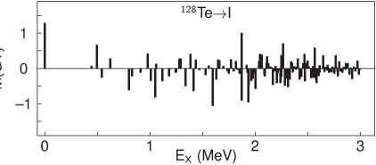
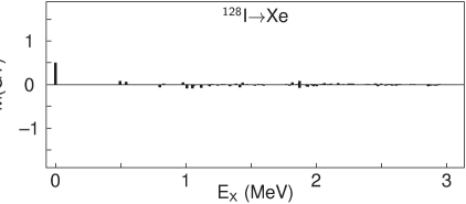
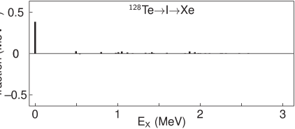
Figure 2: The values of $\langle 1^{+}_{N}||t^{+}\sigma||0^{+}_{1}\rangle$ (top), $\langle 0^{+}_{1}||t^{+}\sigma||1^{+}_{N}\rangle$ (center) and $\langle 0^{+}_{1}||t^{+}\sigma||1^{+}_{N}\rangle\langle 1^{+}_{N}||t^{+}\sigma||0^{+}_{1}\rangle/(\frac{1}{2}(Q_{\beta\beta}+2m_{e}c^{2})+E_{N}-E_{I})$ (bottom), for the double-$\beta$ decay from the lowest $0^{+}$ in ¹²⁸Te to the lowest $0^{+}$ in ¹²⁸Xe through the intermediate $1^{+}$ in ¹²⁸I, plotted as a function of the excitation energy of $1^{+}$.

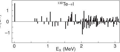
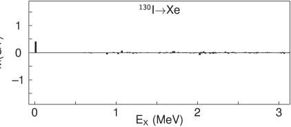
Figure 3: Same plots as Fig. 2 but for ¹³⁰Te decay.

Table 18: The F matrix elements $\langle^{128}\text{Xe}|^{128}\text{I}\rangle$ and $\langle^{128}\text{I}|^{128}\text{Te}\rangle$ and the energies of the $0^{+}_{N}$ states (up to $E_{x}=1.5$ MeV) in ¹²⁸I.

	$\langle^{128}\text{Xe}|^{128}\text{I}\rangle$	$\langle^{128}\text{I}|^{128}\text{Te}\rangle$	128I
$N$	$\langle 0^{+}_{1}|t^{+}|0^{+}_{N}\rangle$	$\langle 0^{+}_{N}|t^{+}|0^{+}_{1}\rangle$	$E_{x}(0^{+}_{N})$
			(MeV)
1	$-$0.0017	0.0836	0.6673
2	$-$0.0497	$-$0.1303	0.7731
3	0.0191	0.1871	0.9547
4	0.0044	0.1475	1.1158
5	$-$0.0256	0.1093	1.3182
6	$-$0.0174	0.3785	1.3382
7	$-$0.0319	0.6042	1.4194
8	0.0041	$-$0.0838	1.4338

Table 19: The F matrix elements $\langle^{130}\text{Xe}|^{130}\text{I}\rangle$ and $\langle^{130}\text{I}|^{130}\text{Te}\rangle$ and the energies of the $0^{+}_{N}$ states (up to $E_{x}=1.5$ MeV) in ¹³⁰I.

	$\langle^{130}\text{Xe}|^{130}\text{I}\rangle$	$\langle^{130}\text{I}|^{130}\text{Te}\rangle$	130I
$N$	$\langle 0^{+}_{1}|t^{+}|0^{+}_{N}\rangle$	$\langle 0^{+}_{N}|t^{+}|0^{+}_{1}\rangle$	$E_{x}(0^{+}_{N})$
			(MeV)
1	0.0245	0.0756	0.8052
2	$-$0.0095	0.0589	0.9045
3	$-$0.0477	0.0466	1.1851
4	$-$0.0136	0.2426	1.2933
5	0.0002	$-$0.0670	1.4032

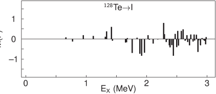
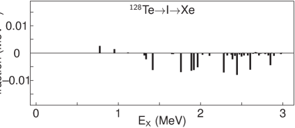
Figure 4: The values of $\langle 0^{+}_{N}||t^{+}||0^{+}_{1}\rangle$ (top), $\langle 0^{+}_{1}||t^{+}||0^{+}_{N}\rangle$ (center) and $\langle 0^{+}_{1}||t^{+}||0^{+}_{N}\rangle\langle 0^{+}_{N}||t^{+}||0^{+}_{1}\rangle/(\frac{1}{2}(Q_{\beta\beta}+2m_{e}c^{2})+E_{N}-E_{I})$ (bottom), for the double-$\beta$ decay from the lowest $0^{+}$ in ¹²⁸Te to the lowest $0^{+}$ in ¹²⁸Xe through the intermediate $0^{+}$ in ¹²⁸I, plotted as a function of the excitation energy of $0^{+}$. Note the small scale in the bottom panel of the figure.

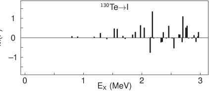
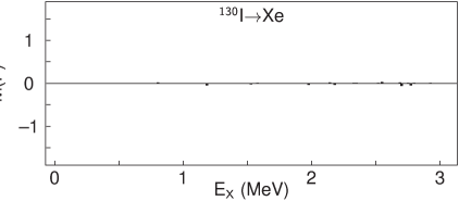
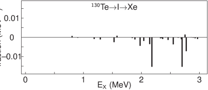
Figure 5: Same as Fig. 4 but for ¹³⁰Te decay.

The strength distribution $B(\text{GT}^{+})=|M(\text{GT})^{+}|^{2}$ for ^128,130Te $\to$ ^128,130I has been measured recently by Puppe et al. [21] by means of the (³He, $t$) reaction. The behavior of the experimental strength distribution is in agreement with the calculated behavior, i.e., the strength appears to be almost uniformly distributed as in our Figures 2 and 3. The authors of [21] extract also the values

$${}^{128}\text{I} B(\text{GT})_{\text{g.s.}}^{(^{3}\text{He},t)} :0.079\;(8), \sum =0.829\;(50)$$ (54)

$${}^{130}\text{I} B(\text{GT})_{\text{g.s.}}^{(^{3}\text{He},t)} :0.072\;(9), \sum =0.746\;(46)$$

where $\sum$ represents the sum of the strength up to 3 MeV. The value 0.079 (8) is in fair agreement with 0.102 (2) obtained from [18, 19] and the value 0.087 (10) calculated by the authors from the data of [22]. From a comparison between the values in (54) and the calculated IBM values

$${}^{128}\text{I} B(\text{GT}) :1.676, \sum =15.09$$ (55)

$${}^{130}\text{I} B(\text{GT}) :2.714, \sum =16.22$$

we can extract the values of $g_{A,\text{eff},(^{3}\text{He},t)}$. We obtain, for ¹²⁸Te ($0^{+}_{1}$) $\to$ ¹²⁸I ($1^{+}_{1}$), $g_{A,\text{eff}}=0.276$ and for ¹³⁰Te ($0^{+}_{1}$) $\to$ ¹³⁰I ($1^{+}_{1}$), $g_{A,\text{eff}}=0.207$. The values so extracted are smaller than those extracted from EC/$\beta^{+}$ and $\beta^{-}$ decay, especially for ¹³⁰Te. This may have to do with the way in which $B(\text{GT})(^{3}\text{He},t)$ is extracted from the cross section, causing a tension between $B(\text{GT})[\text{EC}]=0.102~{}(2)$ and $B(\text{GT})[^{3}\text{He},t]=0.079~{}(8)$ for ¹²⁸I ($1^{+}_{1}$) $\leftrightarrow$ ¹²⁸Te ($0^{+}_{1}$).

If we use the value $g_{A,\text{eff}}=0.28~{}(3)$ obtained from EC/$\beta^{+}$ and $\beta^{-}$ decays, we calculate the quenched values

$${}^{128}\text{I} B(\text{GT})[\text{IBM-quenched}] :0.082, \sum[\text{IBM-quenched}] =0.735$$ (56)

$${}^{130}\text{I} B(\text{GT})[\text{IBM-quenched}] :0.132, \sum[\text{IBM-quenched}] =0.790.$$

The values for ¹²⁸I are in good agreement with the (³He, $t$) values, but only in fair agreement for ¹³⁰I, where we overestimate the summed strength by 5%. We conclude that IBM-quenched calculated values with a single value $g_{A,\text{eff}}=0.28~{}(3)$ provide a good description of all experimental data EC/$\beta^{+}$, $\beta^{-}$ and (³He, $t$) in ¹²⁸I decay, and a fair description of (³He, $t$) in ¹³⁰I decay.

There is no reported measurement of the strength distribution $B(\text{F}^{+})=|M(\text{F})^{+}|^{2}$. In Ref. [21] only the IAS $0^{+}$ state at 11.948 MeV in ¹²⁸I and at 12.718 MeV in ¹³⁰I is identified. However, some excess strength in the region 2–3 MeV, especially around $E_{x}\cong 2.7$ MeV where we predict the F⁺ strength to be concentrated, is seen in Fig. 1 of [21]. It would be of great interest to investigate this point further, since it will clarify the question of isospin violation in this mass region.

3.3 Double-$\beta$ decay

The individual matrix elements of $t^{+}\sigma$ and $t^{+}$ are then combined as in Eqs. (3), (4) and (6) to obtain the matrix elements for $2\nu\beta\beta$ decay. In evaluating the denominators in Eqs. (3), (4) and (6), the following experimental $Q$-values are used: $Q_{\beta}$ (gs) (¹²⁸Te $\to$ ¹²⁸I) = $-1.2518$, $Q_{\beta\beta}$ (gs) (¹²⁸Te $\to$ ¹²⁸Xe) = $0.868$, $Q_{\beta}$ (gs) (¹³⁰Te $\to$ ¹³⁰I) = $-0.420$, $Q_{\beta\beta}$ (gs) (¹³⁰Te $\to$ ¹³⁰Xe) = $2.529$, in units of MeV. When calculating decay to $2^{+}_{1}$ states, we use the experimental values $Q_{\beta\beta}$ ($2^{+}_{1}$) (¹²⁸Te $\to$ ¹²⁸Xe) = 0.425, $Q_{\beta\beta}$ ($2^{+}_{1}$) (¹³⁰Te $\to$ ¹³⁰Xe) = 1.993, also in MeV. The calculated values of $E_{N}$ (exc) in the intermediate odd-odd nucleus and of the individual matrix elements are then combined and summed to give the value of the nuclear matrix elements shown in Table 20. The Fermi matrix elements in this table are a factor of approximately 10 smaller than the Gamow-Teller matrix elements. Introducing the quantity $\chi_{\text{F}}=M_{2\nu}^{\text{F}}/M_{2\nu}^{\text{GT}}$ of Ref. [9], we find, for $0_{1}^{+}\to 0_{1}^{+}$ transitions $\chi_{\text{F}}=-0.119$ in ¹²⁸Te decay and $\chi_{\text{F}}=-0.113$ in ¹³⁰Te decay. If isospin was a good quantum number, $\chi_{\text{F}}=0$. Table 20 indicates that there is a small isospin violation in our wave functions. The individual contributions to the sums are also shown in the bottom panels of Figures 2–5, for ^128,130Te$\to^{128,130}$I$\to^{128,130}$Xe. We find that the GT sum is dominated by the lowest $1^{+}_{1}$ state in ^128,130I. This is the most important result of this paper. Our calculation is consistent with (1) the single state dominance (SSD) hypothesis [23, 24, 25] and (2) the Fermi-surface quasi-particle model of Ejiri [26]. The F sum is very small and receives most of its contribution from two states at $E_{x}=$ 2.179 and 2.701 MeV in ¹³⁰I, and at $E_{x}=$ 2.282 and 2.443 MeV in ¹²⁸I.

Table 20: Nuclear matrix elements $M_{2\nu}^{\text{GT}}$, $M_{2\nu}^{\text{F}}$ of transitions from the ground state of ^128,130Te to some states in ^128,130Xe. The sign of $M_{2\nu}^{\text{GT}}$ is chosen to be positive.

transition	128Te$\to^{128}$Xe	130Te$\to^{130}$Xe
GT
$0^{+}_{1}\to 0^{+}_{1}$	0.297	0.273
$0^{+}_{1}\to 2^{+}_{1}$	0.00718	0.00639
$0^{+}_{1}\to 0^{+}_{2}$		0.668
F
$0^{+}_{1}\to 0^{+}_{1}$	$-$0.0353	$-$0.0309
$0^{+}_{1}\to 0^{+}_{2}$		$-$0.112

The matrix elements

$$|M_{2\nu}|=g_{A}^{2}\biggl{|}M^{\text{GT}}_{2\nu}-\Bigl{(}\frac{g_{V}}{g_{A}}\Bigr{)}^{2}M^{\text{F}}_{2\nu}\biggr{|}$$ (57)

for $0^{+}_{1}\to 0^{+}_{1}$ decay can be extracted from experiment using the observed half-life $\tau^{2\nu}_{1/2}$, Eq. (1). The extracted values are [10] 0.044 (6) for ¹²⁸Te decay and 0.031 (4) for ¹³⁰Te decay. These values should be compared with the calculated values

$$|M_{2\nu}^{\text{calc}}|=g_{A}^{2}\biggl{|}M^{\text{GT}}_{2\nu}-\Bigl{(}\frac{g_{V}}{g_{A}}\Bigr{)}^{2}M^{\text{F}}_{2\nu}\biggr{|}.$$ (58)

From the values in Table 20 and $g_{A}=1.269$, $g_{V}=1$, we have 0.514 for ¹²⁸Te and 0.470 for ¹³⁰Te decay. Under the assumption that $g_{A}$ is quenched to $g_{A,\text{eff},\beta\beta}$ while $(g_{V}/g_{A})$ is not, thus writing

$$|M_{2\nu}^{\text{quenched}}|=g_{A,\text{eff},\beta\beta}^{2}|M_{2\nu}^{\text{calc}}|,$$ (59)

we can extract $g_{A,\text{eff},\beta\beta}=0.293$ for ¹²⁸Te and $g_{A,\text{eff},\beta\beta}=0.257$ for ¹³⁰Te, in fair agreement with the values extracted from single-$\beta$ decay, $g_{A,\text{eff},\beta}=$ 0.313 for ¹²⁸Te$\leftarrow^{128}$I and 0.255 for ¹²⁸I$\to^{128}$Xe.

Assuming that the quenching of $g_{A}$ is the same in both single-$\beta$ and $2\nu\beta\beta$ decay and using the adopted value $g_{A,\text{eff}}=0.28~{}(3)$ of Eq. (52) we obtain the quenched values in Table 21, in reasonable agreement with experiment. It appears from this table that knowledge of single-$\beta$ decays allows one to reliably calculate $2\nu\beta\beta$, as emphasized by Ejiri [26], and thus predict the $2\nu\beta\beta$ half-life in cases where it has not been measured. This statement, however, relies on our assumption leading to Eq. (59). Quenching of matrix elements in a given model calculation arises from two effects: (i) The limited model space in which the calculation is done and (ii) coupling to non-nucleonic degrees of freedom ($\Delta$, N^∗, …). For the second part we expect $g_{A}$ to be quenched and $g_{V}$ not, due to the conserved vector current hypothesis (CVC). For the first part, it is reasonable to expect that both $g_{A}$ and $g_{V}$ be quenched. While for $g_{A}$ there are experimental data to extract $g_{A,\text{eff}}$ from single-$\beta$ decay, as we have done in Sect. 3.2, there are no data to extract $g_{V,\text{eff}}$, and thus our assumption that $g_{V}/g_{A}$ in (59) is unquenched is speculative.

Table 21: Two-neutrino double-$\beta$ decay matrix elements, $|M_{2\nu}|$ in IBFM.

	exp	calc	quenched
128Te	0.044 (6)	0.514	0.040 (8)
130Te	0.031 (4)	0.470	0.037 (8)

Using the values in Table 21 and the phase space factor of [10], $G^{(0)}_{2\nu,0^{+}_{1}\to 0^{+}_{1}}$ (${}^{128}\text{Te}\to^{128}\text{Xe}$) = $0.269\times 10^{-21}$ yr^-1 and $G^{(0)}_{2\nu,0^{+}_{1}\to 0^{+}_{1}}$ (${}^{130}\text{Te}\to^{130}\text{Xe}$) = $1529\times 10^{-21}$ yr^-1, we calculate from $\tau^{-1}=G^{(0)}_{2\nu}|M_{2\nu}^{\text{quenched}}|^{2}$, the half-lives $\tau(^{128}\text{Te})=0.23~{}(9)\times 10^{25}$ yr and $\tau(^{130}\text{Te})=0.48~{}(19)\times 10^{25}$ yr to be compared with the experimental values $0.19\times 10^{25}$ yr (¹²⁸Te) and $0.68\times 10^{21}$ yr (¹³⁰Te).

In addition to matrix elements to $0^{+}_{1}$, we have also calculated matrix elements to $0^{+}_{2}$. This state is located at 1.583 MeV in ¹²⁸Xe and at 1.793 MeV in ¹³⁰Xe. Therefore $Q_{\beta\beta}$ ($0^{+}_{2}$) (¹²⁸Te $\to$ ¹²⁸Xe) = $-0.715$, $Q_{\beta\beta}$ ($0^{+}_{2}$) (¹³⁰Te $\to$ ¹³⁰Xe) = $+0.736$. Decay to $0^{+}_{2}$ is possible for ¹³⁰Te decay, while for ¹²⁸Te decay it is not. The values of the GT and F matrix elements to $0^{+}_{2}$ are also shown in Table 20. They are larger than those to $0^{+}_{1}$ due to the smaller energy denominator in Eqs. (3) and (4). They can be combined as in Eq. (58) to give 1.187. Using the same quenching factor $g_{A,\text{eff}}=0.28~{}(3)$ as before, we obtain $M^{\text{eff},\text{quenched}}_{2\nu}(0^{+}_{1}\to 0^{+}_{2})=0.093~{}(18)$.

$2\nu\beta\beta$ decay to $0^{+}_{2}$ has not been observed in ¹³⁰Te decay. It has so far been observed only in ¹⁰⁰Mo and ¹⁵⁰Nd decay [1]. Our calculation indicates that it may be observed. Using the values of Ref. [10], for $G^{(0)}_{2\nu,0^{+}_{1}\to 0^{+}_{1}}=1529\times 10^{-21}$ yr^-1 and $G^{(0)}_{2\nu,0^{+}_{1}\to 0^{+}_{2}}=0.0757\times 10^{-21}$ yr^-1, and the values $|M_{2\nu}^{\text{eff},\text{quenched}}(0^{+}_{1}\to 0^{+}_{1})|=0.037$ and $|M_{2\nu}^{\text{eff},\text{quenched}}(0^{+}_{1}\to 0^{+}_{2})|=0.093$ we find

$$\frac{\tau_{2\nu}\bigl{(}^{130}\text{Te}(0^{+}_{1})\to^{130}\text{Xe}(0^{+}_{2})\bigr{)}}{\tau_{2\nu}\bigl{(}^{130}\text{Te}(0^{+}_{1})\to^{130}\text{Xe}(0^{+}_{1})\bigr{)}}=3200.$$ (60)

The ratio is of the same order of magnitude of

$$\frac{\tau_{2\nu}\bigl{(}^{128}\text{Te}(0^{+}_{1})\to^{128}\text{Xe}(0^{+}_{1})\bigr{)}}{\tau_{2\nu}\bigl{(}^{130}\text{Te}(0^{+}_{1})\to^{130}\text{Xe}(0^{+}_{1})\bigr{)}}=2790.$$ (61)

It is however far larger than in ¹⁰⁰Mo decay where the observed ratio is [1, 10]

$$\frac{\tau_{2\nu}\bigl{(}^{100}\text{Mo}(0^{+}_{1})\to^{100}\text{Ru}(0^{+}_{2})\bigr{)}}{\tau_{2\nu}\bigl{(}^{100}\text{Mo}(0^{+}_{1})\to^{130}\text{Ru}(0^{+}_{1})\bigr{)}}=70~{}(10)$$ (62)

and thus it may be difficult to observe.

3.4 Sensitivity to parameter assumptions

Single-$\beta$ and double-$\beta$ decays are particularly sensitive to the occupation probabilities $u_{j}$, $v_{j}$ of single-particle orbits, as one can see from Eqs. (14)–(17). To test this sensitivity, we have redone the calculation with another set of single-particle energies, as proposed by Fujita and Ikeda [20], shown in Table 22. This set is rather different from that in Table 5, most notably by the location of the $0g_{7/2}$ level and by the inclusion of the $0h_{9/2}$ proton and $0g_{9/2}$ neutron levels. It does not reproduce accurately spectra of odd-even and odd-odd nuclei in the region, but it is considered here to test the sensitivity to the choice of single particle energies.

Table 22: Single-particle energies taken from Ref. [20].

.

orbit	$0g_{9/2}$	$1d_{5/2}$	$0g_{7/2}$	$2s_{1/2}$	$1d_{3/2}$	$0h_{11/2}$	$0h_{9/2}$
	(MeV)	(MeV)	(MeV)	(MeV)	(MeV)	(MeV)	(MeV)
proton		0.00	$-0.63$	2.40	2.30	2.20	7.70
neutron	$-4.08$	0.00	0.42	1.90	2.20	2.40

With this set we re-calculate the distribution of matrix elements for ^128,130Te$\to$I and ^128,130I$\to$Xe, as shown in Figures 6 and 7 for GT. By comparing with Figures 2 and 3, one can see that the qualitative features, including the single-state dominance, are unchanged. The distribution in the leg ^128,130Te$\to$I is practically unchanged. However, a major change occurs in the magnitude of the GT matrix elements from $1^{+}$ in ^128,130I to ^128,130Xe, which are smaller than in the calculation with the s. p. e. of Table 5. This change results in a reduction of the double-$\beta$ matrix elements $|M_{2\nu}|$ as shown in Table 23. The same situation occurs for the F matrix elements. By repeating the same procedure as in Section 3.2, one can extract the values of $g_{A,\text{eff},\beta}$ and $g_{A,\text{eff},(^{3}\text{He},t)}$ for this set of s. p. e.. For ¹²⁸I ($1^{+}_{1}$)$\to^{128}$Te ($0^{+}_{1}$) decay, $g_{A,\text{eff},\beta}=0.292$, and for ¹²⁸I ($1^{+}_{1}$)$\to^{128}$Xe ($0^{+}_{1}$) decay, $g_{A,\text{eff},\beta}=0.413$. For ¹²⁸Te ($0^{+}_{1}$)$\to^{128}$I ($1^{+}_{1}$) (³He, $t$), one has $g_{A,\text{eff},(^{3}\text{He},t)}=0.257$. These values are somewhat inconsistent with each other. Taken on the average, they lead to a larger value of $g_{A,\text{eff}}=0.321$. By repeating the same procedure as in Section 3.3, one can also extract the values $g_{A,\text{eff},\beta\beta}=0.338$ (¹²⁸Te) and 0.373 (¹³⁰Te). The extracted values of $g_{A,\text{eff},\beta}$ are here also somewhat inconsistent with those extracted from single-$\beta$ decay and (³He, $t$). Nevertheless, assuming $g_{A,\text{eff},2\nu\beta\beta}=g_{A,\text{eff},\beta}$, and using the average value $g_{A,\text{eff}}=0.35~{}(6)$ from single-$\beta$, we obtain the values in Table 24. These are in reasonable agreement with experiment, although the agreement is not as good as with the s. p. e. of [11].

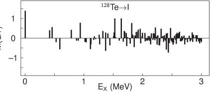
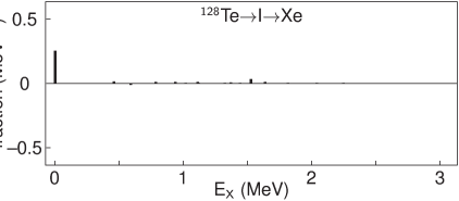
Figure 6: The values of $\langle 1^{+}_{N}||t^{+}\sigma||0^{+}_{1}\rangle$ (top), $\langle 0^{+}_{1}||t^{+}\sigma||1^{+}_{N}\rangle$ (center) and $\langle 0^{+}_{1}||t^{+}\sigma||1^{+}_{N}\rangle\langle 1^{+}_{N}||t^{+}\sigma||0^{+}_{1}\rangle/(\frac{1}{2}(Q_{\beta\beta}+2m_{e}c^{2})+E_{N}-E_{I})$ (bottom) for the double-$\beta$ decay from the lowest $0^{+}$ in ¹²⁸Te to the lowest $0^{+}$ in ¹²⁸Xe calculated by the single-particle energies of [20].

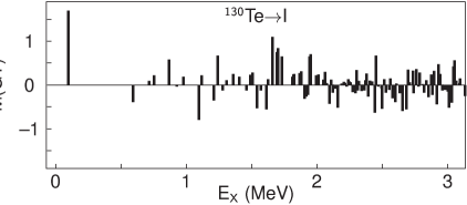
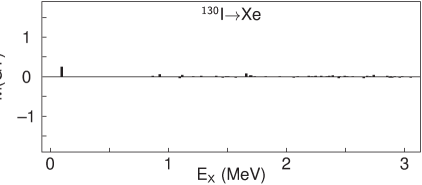
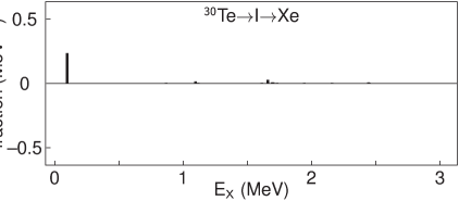
Figure 7: The same plots as Fig. 3 for the decay ¹³⁰Te$\to^{130}$Xe through ¹³⁰I calculated by the single-particle energies of [20].

Table 23: Nuclear matrix elements $M_{2\nu}$ of the transitions from the ground states of ^128,130Te to some states in ^128,130Xe calculated with the single-particle energies of [20].

transition	128Te$\to^{128}$Xe	130Te$\to^{130}$Xe
GT
$0^{+}_{1}\to 0^{+}_{1}$	0.178	0.152
$0^{+}_{1}\to 2^{+}_{1}$	0.00334	0.00201
$0^{+}_{1}\to 0^{+}_{2}$		0.557
F
$0^{+}_{1}\to 0^{+}_{1}$	$-0.0297$	$-0.0268$
$0^{+}_{1}\to 0^{+}_{2}$		$-0.110$

Table 24: Two-neutrino double-$\beta$ decay matrix elements, $|M_{2\nu}|$ in IBFM with single particle energies of [20].

	exp	calc	quenched
128Te	0.044 (6)	0.315	0.039 (13)
130Te	0.031 (4)	0.271	0.033 (11)

3.5 Sensitivity to truncation to $E_{x}<3$ MeV

The calculations reported in the previous subsections are based on contributions of states in the intermediate odd-odd nucleus with $E_{x}<3$ MeV. It is of interest to investigate how likely or unlikely is that states above 3 MeV could contribute significantly to two-neutrino decay.

The $1^{+}$ and $0^{+}$ states with $E_{x}>3$ MeV are built from two contributions: (1) states constructed from single-particle orbitals within the model space of Table 5; (2) states constructed from single-particle orbitals above the shell gap at 82 or below the shell gap at 50. To investigate the contribution of states with $E_{x}>3$ MeV within the model space of Table 5, one can simply extend the calculation from the current lowest $\sim 100$ $1^{+}$ states and $\sim 50$ $0^{+}$ states to larger numbers. It appears that the properties of the strength distributions remain the same and that therefore states of this type will not contribute significantly to two-neutrino decay. States constructed from single-particle orbits outside the model space of Table 5 will appear in the spectrum at energies above the shell gaps, $E_{x}\gtrsim 5$ MeV. We have in fact investigated their contributions by including the proton orbit $0h_{9/2}$ and the neutron orbit $0g_{9/2}$, as in Table 22, and concluded that also this type of states will not contribute significantly to two-neutrino decay. The argument is as follows. Inclusion of excitations across major shells will give major contributions to the strength distribution for the GT^- and F^- “legs”, Te $\to$ I, especially in the region $E_{x}\geqslant 10$ MeV, where the giant GT resonance ($E_{x}\simeq 14$ MeV) and the Isobaric Analogue State, IAS ($E_{x}\simeq 12$ MeV) are located. However, because of their composition in terms of single-particle states, we expect its contribution to the GT⁺ (or F⁺) “leg”, I $\to$ Xe, which will still remain concentrated in few low-lying states, Figs. 6 and 7, center panel. It is therefore, in our opinion, quite unlikely that states above 3 MeV will contribute significantly to two-neutrino decay.

4 Conclusion

In this article, a detailed investigation of the ten nuclei: ^128,130Te, ^128,130I, ^128,130Xe, ^129,131I and ^127,129Te, within the framework of the interacting boson model-2, IBM-2, and its generalizations IBFM-2 and IBFFM-2 has been done. The parameters needed in this investigation have been obtained as much as possible from the available experimental information. The wave functions so obtained have been used to calculate single-$\beta$ and $2\nu\beta\beta$ matrix elements.

The main results of our investigation are:

1. The mechanism of $2\nu\beta\beta$ in these nuclei appears to be single-state dominance (SSD).

2. The GT strength in ^128,130Te ($0^{+}_{1}$) $\to$ ^128,130I ($1^{+}_{N}$) is evenly distributed.

3. The GT strength in ^128,130I ($1^{+}_{N}$) $\to$ ^128,130Xe ($0^{+}_{1}$) is concentrated in one state.

4. Use of a single value $g_{A,\text{eff}}\equiv g_{A,\text{eff},\beta}\equiv g_{A,\text{eff},\beta\beta}$ appears to describe well both single-$\beta$ and $2\nu\beta\beta$ decay.

5. The results are very sensitive to the choice of single-particle energies, most notably the weak branch ${}^{128,130}\text{I}\to^{128,130}\text{Xe}$. However, when the renormalization of $g_{A}$ is taken into account through fitting the single-$\beta$ decay, different choices of s. p. e. give similar results for $2\nu\beta\beta$, but with varying degree of accuracy. The best choice appears to be that of the s. p. e. of [11] which describes all observed quantities fairly: energies, electromagnetic transitions and moments, single-$\beta$ matrix elements, (³He, $t$) strength distributions, and double-$\beta$ matrix elements, in the quenched approximation.

Our best estimates of $2\nu\beta\beta$ matrix elements are therefore those given in Table 21, $|M_{2\nu}^{\text{eff}}|=0.040~{}(8)$ for ${}^{128}\text{Te}(0^{+}_{1})\to^{128}\text{Xe}(0^{+}_{1})$ and $|M_{2\nu}^{\text{eff}}|=0.037~{}(8)$ for ${}^{130}\text{Te}(0^{+}_{1})\to^{130}\text{Xe}(0^{+}_{1})$, and of the $2\nu\beta\beta$ half-lives $\tau$ (${}^{128}\text{Te})=0.23~{}(9)\times 10^{25}$ yr, $\tau$ (${}^{130}\text{Te})=0.48~{}(19)\times 10^{21}$ yr.

Our extracted values $g_{A,\text{eff}}=0.28~{}(3)$ and $g_{A,\text{eff}}=0.35~{}(6)$ for the single-particle levels of Table 5 and 22, respectively, are rather low. The values of $g_{A,\text{eff}}$ depend on mass number, $A$, and on the nuclear model used in their extraction. A preliminary study of $g_{A,\text{eff}}$ in the Interacting Boson Model (IBM-2) in the closure approximation for $2\nu\beta\beta$ decay and the Interacting Shell Model (ISM) has been done in [30]. It has been found that $g_{A,\text{eff}}$ has a smooth dependence that can be parametrized as $g_{A,\text{eff}}=1.269A^{-0.18}$ plus shell effects. The extracted values of $g_{A.\text{eff}}$ in the mass region, $A\sim 130$, are $g_{A,\text{eff}}\simeq 0.5$ for IBM-2 and $\sim 0.6$ for ISM. A similar analysis has been done within the framework of QRPA [31] with similar results. We intend to continue the study of $g_{A,\text{eff}}$ within the framework described in the present article to understand how general is the result presented here, and also to study the related question of the extent to which $g_{V}$ is quenched in heavy nuclei, if at all.

The question of the impact of the small value of $g_{A,\text{eff}}$ found in $\beta$-decay and $2\nu\beta\beta$-decay to $0\nu\beta\beta$-decay is the subject of much debate. While only GT ($1^{+}$) and F ($0^{+}$) multipoles contribute to allowed $\beta$- and $2\nu\beta\beta$-decay, all multipoles ($1^{+},2^{-},3^{+},$ …), ($0^{+},1^{-},2^{+},$ …) contribute to $0\nu\beta\beta$ decay. It is not clear whether or not the higher multipoles are quenched. Nonetheless, since $1^{+}$ and $0^{+}$ still provide the largest contributions, we expect the quenching of $g_{A}$ and $g_{V}$ to play an important role in $0\nu\beta\beta$ decay. Since, in view of the fact that $g_{A}$ appears to the fourth power in the decay rate, the quenching of $g_{A}$ has major repercussions on $0\nu\beta\beta$ experiments, we plan to investigate this problem in depth in subsequent papers.

References

- [1] For a review, see, A. S. Barabash, Phys. Rev. C 81,035501 (2010).
- [2] For reviews, see, J. Suhonen and O. Civitarese, Phys. Rep., 300, 123 (1998); A. Faessler and F. Šimkovic, J. Phys. C 24,2139,(1998).
- [3] E. Caurier, F. Nowacki, and A. Poves, Int. J. Mod. Phys. E, 16, 552 (2007).
- [4] F. Iachello and P. Van Isacker, The interacting boson-fermion model, (Cambridge University Press, Cambridge, 1991).
- [5] S. Brant, N. Yoshida, and L. Zuffi, Phys. Rev. C, 24, 024303 (2006); N. Yoshida, L. Zuffi and S. Brant, Int. J. Mod. Phys. E, 15, 1933 (2006).
- [6] M. Doi, T. Kotani, H. Nishiura, K. Okuda, and E. Takasugi, Prog. Theor. Phys. 66, 1739 (1982).
- [7] M. Doi, T. Kotani, H.Nishiura, and E. Takasugi, Prog. Theor. Phys. 69, 602 (1983).
- [8] F. Boehm and P. Vogel, Physics of Massive Neutrinos, (Cambridge University Press, Cambridge, 1987).
- [9] T. Tomoda, Rep. Prog. Phys., 54, 53 (1991).
- [10] J. Kotila and F. Iachello, Phys. Rev. C, 85, 034316 (2012).
- [11] F. Dellagiacoma, Ph.D. thesis, Yale University, 1988.
- [12] F. Dellagiacoma and F. Iachello, Phys. Lett. B, 218, 399 (1989).
- [13] G. Puddu, O. Scholten, and T. Otsuka, Nucl. Phys. A 348, 109 (1980).
- [14] O. Scholten, Ph. D. thesis, University of Groningen, The Netherlands, 1980.
- [15] S. Brant and V. Paar, Z. Phys., 329, 151 (1988).
- [16] P. J. Brussaard and P. W. M. Glaudemans, Shell-model applications in nuclear spectroscopy, (North-Holland Publishing, Amsterdam, 1977).
- [17] K. Nakamura et al. (Particle Data Group) J. Phys. G, 37, 07502, (2010).
- [18] M. Kanbe, K. Kitao, Nucl. Data Sheets, 94, 227 (2001).
- [19] Balraj Singh, Nucl. Data Sheets, 93, 33 (2001).
- [20] J.-I. Fujita and K. Ikeda, Nucl. Phys. 67, 145, (1965).
- [21] P. Puppe et al. Phys. Rev. C, 86, 044603 (201).
- [22] H. Miyahara, H. Matumoto, G. Wurdiyanto, K. Yanagida, Y. Takenaka, A. Yoshida, and C. Mori, Nucl. Instrum. Meth. Phys. Res. Sec. A, 353, 229 (1994).
- [23] J. Abad, A. Morales, R. Núñez-Lagos, and A. F. Pacheco, Au. Fis. A, 80, 9 (1984).
- [24] A. Griffiths and P. Vogel, Phys. Rev. C,46, 181 (1992).
- [25] O. Civitarese and J.Suhonen, Phys. Rev. C, 58, 1535 (1998).
- [26] H. Ejiri, Prog. Part. Nucl. Phys., 64, 249 (2010).
- [27] J. Suhonen and O. Civitarese, Phys. Lett. B, 668, 277 (2008).
- [28] J. P. Schiffer et al. Phys. Rev. Lett. 100, 112501 (2008).
- [29] B. P. Kay et al. Phys. Rev. C, 79, 021301(R) (2009).
- [30] J. Barea, J. Kotila, and F. Iachello, Phys. Rev. C, 87, 014315 (2013).
- [31] A. Faessler, G. L. Fogli, E. Lisi, V. Rodin, A. M. Rotunno, and F. Šimkovic, J. Phys. G: Nucl. Part. Phys., 35, 075104 (2008).