A significance test for the lasso

Abstract

In the sparse linear regression setting, we consider testing the significance of the predictor variable that enters the current lasso model, in the sequence of models visited along the lasso solution path. We propose a simple test statistic based on lasso fitted values, called the covariance test statistic, and show that when the true model is linear, this statistic has an $\operatorname{Exp}(1)$ asymptotic distribution under the null hypothesis (the null being that all truly active variables are contained in the current lasso model). Our proof of this result for the special case of the first predictor to enter the model (i.e., testing for a single significant predictor variable against the global null) requires only weak assumptions on the predictor matrix $X$. On the other hand, our proof for a general step in the lasso path places further technical assumptions on $X$ and the generative model, but still allows for the important high-dimensional case $p>n$, and does not necessarily require that the current lasso model achieves perfect recovery of the truly active variables.

Of course, for testing the significance of an additional variable between two nested linear models, one typically uses the chi-squared test, comparing the drop in residual sum of squares (RSS) to a $\chi^{2}_{1}$ distribution. But when this additional variable is not fixed, and has been chosen adaptively or greedily, this test is no longer appropriate: adaptivity makes the drop in RSS stochastically much larger than $\chi^{2}_{1}$ under the null hypothesis. Our analysis explicitly accounts for adaptivity, as it must, since the lasso builds an adaptive sequence of linear models as the tuning parameter $\lambda$ decreases. In this analysis, shrinkage plays a key role: though additional variables are chosen adaptively, the coefficients of lasso active variables are shrunken due to the $\ell_{1}$ penalty. Therefore, the test statistic (which is based on lasso fitted values) is in a sense balanced by these two opposing properties—adaptivity and shrinkage—and its null distribution is tractable and asymptotically $\operatorname{Exp}(1)$.

T11Discussed in d10.1214/13-AOS1175A, d10.1214/13-AOS1175B, d10.1214/13-AOS1175C, d10.1214/13-AOS1175D, d10.1214/13-AOS1175E and d10.1214/14-AOS1175F; rejoinder at r10.1214/14-AOS1175REJ.

, ,
and t1Supported by the Natural Sciences and Engineering Research Council of Canada. t2Supported by NSF Grant DMS-12-08857 and AFOSR Grant 113039. t3Supported by NSF Grant DMS-13-09174. t4Supported by NSF Grant DMS-99-71405 and NIH Grant EB-001988. A significance test for the lasso

1 Introduction.

We consider the usual linear regression setup, for an outcome vector $y\in\mathbb{R}^{n}$ and matrix of predictor variables $X\in\mathbb{R}^{n\times p}$:

$$y=X\beta^{*}+\varepsilon,\qquad\varepsilon\sim N\bigl{(}0,\sigma^{2}I\bigr{)},$$ (1)

where $\beta^{*}\in\mathbb{R}^{p}$ are unknown coefficients to be estimated. [If an intercept term is desired, then we can still assume a model of the form (1) after centering $y$ and the columns of $X$; see Section 2.2 for more details.] We focus on the lasso estimator [Tibshirani (1996), Chen, Donoho and Saunders (1998)], defined as

$$\hat{\beta}=\mathop{\operatorname{argmin}}_{\beta\in\mathbb{R}^{p}}\frac{1}{2}\|y-X\beta\|_{2}^{2}+\lambda\|\beta\|_{1},$$ (2)

where $\lambda\geq 0$ is a tuning parameter, controlling the level of sparsity in $\hat{\beta}$. Here, we assume that the columns of $X$ are in general position in order to ensure uniqueness of the lasso solution [this is quite a weak condition, to be discussed again shortly; see also Tibshirani (2013)].

There has been a considerable amount of recent work dedicated to the lasso problem, both in terms of computation and theory. A comprehensive summary of the literature in either category would be too long for our purposes here, so we instead give a short summary: for computational work, some relevant contributions are Friedman et al. (2007), Beck and Teboulle (2009), Friedman, Hastie and Tibshirani (2010), Becker, Bobin and Candès (2011), Boyd et al. (2011), Becker, Candès and Grant (2011); and for theoretical work see, for example, Greenshtein and Ritov (2004), Fuchs (2005), Donoho (2006), Candes and Tao (2006), Zhao and Yu (2006), Wainwright (2009), Candès and Plan (2009). Generally speaking, theory for the lasso is focused on bounding the estimation error $\|X\hat{\beta}-X\beta^{*}\|_{2}^{2}$ or $\|\hat{\beta}-\beta^{*}\|_{2}^{2}$, or ensuring exact recovery of the underlying model, $\operatorname{supp}(\hat{\beta})=\operatorname{supp}(\beta^{*})$ [with $\operatorname{supp}(\cdot)$ denoting the support function]; favorable results in both respects can be shown under the right assumptions on the generative model (1) and the predictor matrix $X$. Strong theoretical backing, as well as fast algorithms, have made the lasso a highly popular tool.

Yet, there are still major gaps in our understanding of the lasso as an estimation procedure. In many real applications of the lasso, a practitioner will undoubtedly seek some sort of inferential guarantees for his or her computed lasso model—but, generically, the usual constructs like $p$-values, confidence intervals, etc., do not exist for lasso estimates. There is a small but growing literature dedicated to inference for the lasso, and important progress has certainly been made, with many methods being based on resampling or data splitting; we review this work in Section 2.5. The current paper focuses on a significance test for lasso models that does not employ resampling or data splitting, but instead uses the full data set as given, and proposes a test statistic that has a simple and exact asymptotic null distribution.

Section 2 defines the problem that we are trying to solve, and gives the details of our proposal—the covariance test statistic. Section 3 considers an orthogonal predictor matrix $X$, in which case the statistic greatly simplifies. Here, we derive its $\operatorname{Exp}(1)$ asymptotic distribution using relatively simple arguments from extreme value theory. Section 4 treats a general (nonorthogonal) $X$, and under some regularity conditions, derives an $\operatorname{Exp}(1)$ limiting distribution for the covariance test statistic, but through a different method of proof that relies on discrete-time Gaussian processes. Section 5 empirically verifies convergence of the null distribution to $\operatorname{Exp}(1)$ over a variety of problem setups. Up until this point, we have assumed that the error variance $\sigma^{2}$ is known; in Section 6, we discuss the case of unknown $\sigma^{2}$. Section 7 gives some real data examples. Section 8 covers extensions to the elastic net, generalized linear models, and the Cox model for survival data. We conclude with a discussion in Section 9.

2 Significance testing in linear modeling.

Classic theory for significance testing in linear regression operates on two fixed nested models. For example, if $M$ and $M\cup\{j\}$ are fixed subsets of $\{1,\ldots,p\}$, then to test the significance of the $j$th predictor in the model (with variables in) $M\cup\{j\}$, one naturally uses the chi-squared test, which computes the drop in residual sum of squares (RSS) from regression on $M\cup\{j\}$ and $M$,

$$R_{j}=(\mathrm{RSS}_{M}-\mathrm{RSS}_{M\cup\{j\}})/\sigma^{2}$$ (3)

and compares this to a $\chi_{1}^{2}$ distribution. (Here, $\sigma^{2}$ is assumed to be known; when $\sigma^{2}$ is unknown, we use the sample variance in its place, which results in the $F$-test, equivalent to the $t$-test, for testing the significance of variable $j$.)

Often, however, one would like to run the same test for $M$ and $M\cup\{j\}$ that are not fixed, but the outputs of an adaptive or greedy procedure. Unfortunately, adaptivity invalidates the use of a $\chi_{1}^{2}$ null distribution for the statistic (3). As a simple example, consider forward stepwise regression: starting with an empty model $M=\varnothing$, we enter predictors one at a time, at each step choosing the predictor $j$ that gives the largest drop in residual sum of squares. In other words, forward stepwise regression chooses $j$ at each step in order to maximize $R_{j}$ in (3), over all $j\notin M$. Since $R_{j}$ follows a $\chi_{1}^{2}$ distribution under the null hypothesis for each fixed $j$, the maximum possible $R_{j}$ will clearly be stochastically larger than $\chi_{1}^{2}$ under the null. Therefore, using a chi-squared test to evaluate the significance of a predictor entered by forward stepwise regression would be far too liberal (having type I error much larger than the nominal level). Figure 1(a) demonstrates this point by displaying the quantiles of $R_{1}$ in forward stepwise regression (the chi-squared statistic for the first predictor to enter) versus those of a $\chi_{1}^{2}$ variate, in the fully null case (when $\beta^{*}=0$). A test at the $5\%$ level, for example, using the $\chi^{2}_{1}$ cutoff of $3.84$, would have an actual type I error of about $39\%$.

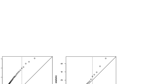
Figure 1: A simple example with $n=100$ observations and $p=10$ orthogonal predictors. All true regression coefficients are zero, $\beta^{*}=0$. On the left is a quantile–quantile plot, constructed over 1000 simulations, of the standard chi-squared statistic $R_{1}$ in (3), measuring the drop in residual sum of squares for the first predictor to enter in forward stepwise regression, versus the $\chi_{1}^{2}$ distribution. The dashed vertical line marks the 95% quantile of the $\chi_{1}^{2}$ distribution. The right panel shows a quantile–quantile plot of the covariance test statistic $T_{1}$ in (5) for the first predictor to enter in the lasso path, versus its asymptotic null distribution $\operatorname{Exp}(1)$. The covariance test explicitly accounts for the adaptive nature of lasso modeling, whereas the usual chi-squared test is not appropriate for adaptively selected models, for example, those produced by forward stepwise regression.

The failure of standard testing methodology when applied to forward stepwise regression is not an anomaly—in general, there seems to be no direct way to carry out the significance tests designed for fixed linear models in an adaptive setting. Our aim is hence to provide a (new) significance test for the predictor variables chosen adaptively by the lasso, which we describe next.

2.1 The covariance test statistic.

The test statistic that we propose here is constructed from the lasso solution path, that is, the solution $\hat{\beta}(\lambda)$ in (2) a function of the tuning parameter $\lambda\in[0,\infty)$. The lasso path can be computed by the well-known LARS algorithm of Efron et al. (2004) [see also Osborne, Presnell and Turlach (2000a, 2000b)], which traces out the solution as $\lambda$ decreases from $\infty$ to $0$. Note that when $\operatorname{rank}(X)<p$ there are possibly many lasso solutions at each $\lambda$ and, therefore, possibly many solution paths; we assume that the columns of $X$ are in general position, implying that there is a unique lasso solution at each $\lambda>0$, and hence a unique path. The assumption that $X$ has columns in general position is a very weak one [much weaker, e.g., than assuming that $\operatorname{rank}(X)=p$]. For example, if the entries of $X$ are drawn from a continuous probability distribution on $\mathbb{R}^{np}$, then the columns of $X$ are almost surely in general position, and this is true regardless of the sizes of $n$ and $p$; see Tibshirani (2013).

Before defining our statistic, we briefly review some properties of the lasso path.

• The path $\hat{\beta}(\lambda)$ is a continuous and piecewise linear function of $\lambda$, with knots (changes in slope) at values $\lambda_{1}\geq\lambda_{2}\geq\cdots\geq\lambda_{r}\geq 0$ (these knots depend on $y,X$).

• At $\lambda=\infty$, the solution $\hat{\beta}(\infty)$ has no active variables (i.e., all variables have zero coefficients); for decreasing $\lambda$, each knot $\lambda_{k}$ marks the entry or removal of some variable from the current active set (i.e., its coefficient becomes nonzero or zero, resp.). Therefore, the active set, and also the signs of active coefficients, remain constant in between knots.

• At any point $\lambda$ in the path, the corresponding active set $A=\operatorname{supp}(\hat{\beta}(\lambda))$ of the lasso solution indexes a linearly independent set of predictor variables, that is, $\operatorname{rank}(X_{A})=|A|$, where we use $X_{A}$ to denote the columns of $X$ in $A$.

• For a general $X$, the number of knots in the lasso path is bounded by $3^{p}$ (but in practice this bound is usually very loose). This bound comes from the following realization: if at some knot $\lambda_{k}$, the active set is $A=\operatorname{supp}(\hat{\beta}(\lambda_{k}))$ and the signs of active coefficients are $s_{A}=\operatorname{sign}(\hat{\beta}_{A}(\lambda_{k}))$, then the active set and signs cannot again be $A$ and $s_{A}$ at some other knot $\lambda_{\ell}\neq\lambda_{k}$. This in particular means that once a variable enters the active set, it cannot immediately leave the active set at the next step.

• For a matrix $X$ satisfying the positive cone condition (a restrictive condition that covers, e.g., orthogonal matrices), there are no variables removed from the active set as $\lambda$ decreases and, therefore, the number of knots is $p$.

We can now precisely define the problem that we are trying to solve: at a given step in the lasso path (i.e., at a given knot), we consider testing the significance of the variable that enters the active set. To this end, we propose a test statistic defined at the $k$th step of the path.

First, we define some needed quantities. Let $A$ be the active set just before $\lambda_{k}$, and suppose that predictor $j$ enters at $\lambda_{k}$. Denote by $\hat{\beta}(\lambda_{k+1})$ the solution at the next knot in the path $\lambda_{k+1}$, using predictors $A\cup\{j\}$. Finally, let $\tilde{\beta}_{A}(\lambda_{k+1})$ be the solution of the lasso problem using only the active predictors $X_{A}$, at $\lambda=\lambda_{k+1}$. To be perfectly explicit,

$$\tilde{\beta}_{A}(\lambda_{k+1})=\mathop{\operatorname{argmin}}_{\beta_{A}\in\mathbb{R}^{|A|}}\frac{1}{2}\|y-X_{A}\beta_{A}\|_{2}^{2}+\lambda_{k+1}\|\beta_{A}\|_{1}.$$ (4)

We propose the covariance test statistic defined by

$$T_{k}=\bigl{(}\bigl{\langle}y,X\hat{\beta}(\lambda_{k+1})\bigr{\rangle}-\bigl{\langle}y,X_{A}\tilde{\beta}_{A}(\lambda_{k+1})\bigr{\rangle}\bigr{)}/\sigma^{2}.$$ (5)

Intuitively, the covariance statistic in (5) is a function of the difference between $X\hat{\beta}$ and $X_{A}\tilde{\beta}_{A}$, the fitted values given by incorporating the $j$th predictor into the current active set, and leaving it out, respectively. These fitted values are parameterized by $\lambda$, and so one may ask: at which value of $\lambda$ should this difference be evaluated? Well, note first that $\tilde{\beta}_{A}(\lambda_{k})=\hat{\beta}_{A}(\lambda_{k})$, that is, the solution of the reduced problem at $\lambda_{k}$ is simply that of the full problem, restricted to the active set $A$ (as verified by the KKT conditions). Clearly then, this means that we cannot evaluate the difference at $\lambda=\lambda_{k}$, as the $j$th variable has a zero coefficient upon entry at $\lambda_{k}$, and hence

$$X\hat{\beta}(\lambda_{k})=X_{A}\hat{\beta}_{A}(\lambda_{k})=X_{A}\tilde{\beta}_{A}(\lambda_{k}).$$

Indeed, the natural choice for the tuning parameter in (5) is $\lambda=\lambda_{k+1}$: this allows the $j$th coefficient to have its fullest effect on the fit $X\hat{\beta}$ before the entry of the next variable at $\lambda_{k+1}$ (or possibly, the deletion of a variable from $A$ at $\lambda_{k+1}$).

Secondly, one may also ask about the particular choice of function of $X\hat{\beta}(\lambda_{k+1})-X_{A}\tilde{\beta}_{A}(\lambda_{k+1})$. The covariance statistic in (5) uses an inner product of this difference with $y$, which can be roughly thought of as an (uncentered) covariance, hence explaining its name. At a high level, the larger the covariance of $y$ with $X\hat{\beta}$ compared to that with $X_{A}\tilde{\beta}_{A}$, the more important the role of variable $j$ in the proposed model $A\cup\{j\}$. There certainly may be other functions that would seem appropriate here, but the covariance form in (5) has a distinctive advantage: this statistic admits a simple and exact asymptotic null distribution. In Sections 3 and 4, we show that under the null hypothesis that the current lasso model contains all truly active variables, $A\supseteq\operatorname{supp}(\beta^{*})$,

$$T_{k}\stackrel{{\scriptstyle d}}{{\rightarrow}}\operatorname{Exp}(1),$$

that is, $T_{k}$ is asymptotically distributed as a standard exponential random variable, given reasonable assumptions on $X$ and the magnitudes of the nonzero true coefficients. [In some cases, e.g., when we have a strict inclusion $A\supsetneq\operatorname{supp}(\beta^{*})$, the use of an $\operatorname{Exp}(1)$ null distribution is actually conservative, because the limiting distribution of $T_{k}$ is stochastically smaller than $\operatorname{Exp}(1)$.] In the above limit, we are considering both $n,p\rightarrow\infty$; in Section 4, we allow for the possibility $p>n$, the high-dimensional case.

See Figure 1(b) for a quantile–quantile plot of $T_{1}$ versus an $\operatorname{Exp}(1)$ variate for the same fully null example ($\beta^{*}=0$) used in Figure 1(a); this shows that the weak convergence to $\operatorname{Exp}(1)$ can be quite fast, as the quantiles are decently matched even for $p=10$. Before proving this limiting distribution in Sections 3 (for an orthogonal $X$) and 4 (for a general $X$), we give an example of its application to real data, and discuss issues related to practical usage. We also derive useful alternative expressions for the statistic, present a connection to degrees of freedom, review related work, and finally, discuss the null hypothesis in more detail.

2.2 Prostate cancer data example and practical issues.

We consider a training set of 67 observations and 8 predictors, the goal being to predict log of the PSA level of men who had surgery for prostate cancer. For more details, see Hastie, Tibshirani and Friedman (2008) and the references therein. Table 1 shows the results of forward stepwise regression and the lasso. Both methods entered the same predictors in the same order. The forward stepwise $p$-values are smaller than the lasso $p$-values, and would enter four predictors at level $0.05$. The latter would enter only one or maybe two predictors. However, we know that the forward stepwise $p$-values are inaccurate, as they are based on a null distribution that does not account for the adaptive choice of predictors. We now make several remarks.

=270pt Step Predictor entered Forward stepwise Lasso 1 lcavol 0.000 0.000 2 lweight 0.000 0.052 3 svi 0.041 0.174 4 lbph 0.045 0.929 5 pgg45 0.226 0.353 6 age 0.191 0.650 7 lcp 0.065 0.051 8 gleason 0.883 0.978

Table 1: Forward stepwise and lasso applied to the prostate cancer data example. The error variance is estimated by $\hat{\sigma}^{2}$, the MSE of the full model. Forward stepwise regression $p$-values are based on comparing the drop in residual sum of squares (divided by $\hat{\sigma}^{2}$) to an $F(1,n-p)$ distribution (using $\chi^{2}_{1}$ instead produced slightly smaller $p$-values). The lasso $p$-values use a simple modification of the covariance test (5) for unknown variance, given in Section 6. All $p$-values are rounded to 3 decimal places

Remark 1.

The above example implicitly assumed that one might stop entering variables into the model when the computed $p$-value rose above some threshold. More generally, our proposed test statistic and associated $p$-values could be used as the basis for multiple testing and false discovery rate control methods for this problem; we leave this to future work.

Remark 2.

In the example, the lasso entered a predictor into the active set at each step. For a general $X$, however, a given predictor variable may enter the active set more than once along the lasso path, since it may leave the active set at some point. In this case, we treat each entry as a separate problem. Our test is specific to a step in the path, and not to a predictor variable at large.

Remark 3.

For the prostate cancer data set, it is important to include an intercept in the model. To accommodate this, we ran the lasso on centered $y$ and column-centered $X$ (which is equivalent to including an unpenalized intercept term in the lasso criterion), and then applied the covariance test (with the centered data). In general, centering $y$ and the columns of $X$ allows us to account for the effect of an intercept term, and still use a model of the form (1). From a theoretical perspective, this centering step creates a weak dependence between the components of the error vector $\varepsilon\in\mathbb{R}^{n}$. If originally we assumed i.i.d. errors, $\varepsilon_{i}\sim N(0,\sigma^{2})$, then after centering $y$ and the columns of $X$, our new errors are of the form $\tilde{\varepsilon}_{i}=\varepsilon_{i}-\bar{\varepsilon}$, where $\bar{\varepsilon}=\sum_{j=1}^{n}\varepsilon_{j}/n$. It is easy see that these new errors are correlated:

$$\operatorname{Cov}(\tilde{\varepsilon}_{i},\tilde{\varepsilon}_{j})=-\sigma^{2}/n\qquad\mbox{for }i\neq j.$$

One might imagine that such correlation would cause problems for our theory in Sections 3 and 4, which assumes i.i.d. normal errors in the model (1). However, a careful look at the arguments in these sections reveals that the only dependence on $y$ is through $X^{T}y$, the inner products of $y$ with the columns of $X$. Furthermore,

$$\operatorname{Cov}\bigl{(}X_{i}^{T}\tilde{\varepsilon},X_{j}^{T}\tilde{\varepsilon}\bigr{)}=\sigma^{2}X_{i}^{T}\biggl{(}I-\frac{1}{n}\mathbh{1}\mathbh{1}^{T}\biggr{)}X_{j}=\sigma^{2}X_{i}^{T}X_{j}\qquad\mbox{for all }i,j,$$

which is the same as it would have been without centering (here $\mathbh{1}\mathbh{1}^{T}$ is the matrix of all $1$s, and we used that the columns of $X$ are centered). Therefore, our arguments in Sections 3 and 4 apply equally well to centered data, and centering has no effect on the asymptotic distribution of $T_{k}$.

Remark 4.

By design, the covariance test is applied in a sequential manner, estimating $p$-values for each predictor variable as it enters the model along the lasso path. A more difficult problem is to test the significance of any of the active predictors in a model fit by the lasso, at some arbitrary value of the tuning parameter $\lambda$. We discuss this problem briefly in Section 9.

2.3 Alternate expressions for the covariance statistic.

Here, we derive two alternate forms for the covariance statistic in (5). The first lends some insight into the role of shrinkage, and the second is helpful for the convergence results that we establish in Sections 3 and 4. We rely on some basic properties of lasso solutions; see, for example, Tibshirani and Taylor (2012), Tibshirani (2013). To remind the reader, we are assuming that $X$ has columns in general position.

For any fixed $\lambda$, if the lasso solution has active set $A=\operatorname{supp}(\hat{\beta}(\lambda))$ and signs $s_{A}=\operatorname{sign}(\hat{\beta}_{A}(\lambda))$, then it can be written explicitly (over active variables) as

$$\hat{\beta}_{A}(\lambda)=\bigl{(}X_{A}^{T}X_{A}\bigr{)}^{-1}X_{A}^{T}y-\lambda\bigl{(}X_{A}^{T}X_{A}\bigr{)}^{-1}s_{A}.$$

In the above expression, the first term $(X_{A}^{T}X_{A})^{-1}X_{A}^{T}y$ simply gives the regression coefficients of $y$ on the active variables $X_{A}$, and the second term $-\lambda(X_{A}^{T}X_{A})^{-1}s_{A}$ can be thought of as a shrinkage term, shrinking the values of these coefficients toward zero. Further, the lasso fitted value at $\lambda$ is

$$X\hat{\beta}(\lambda)=P_{A}y-\lambda\bigl{(}X_{A}^{T}\bigr{)}^{+}s_{A},$$ (6)

where $P_{A}=X_{A}(X_{A}^{T}X_{A})^{-1}X_{A}^{T}$ denotes the projection onto the column space of $X_{A}$, and $(X_{A}^{T})^{+}=X_{A}(X_{A}^{T}X_{A})^{-1}$ is the (Moore–Penrose) pseudoinverse of $X_{A}^{T}$.

Using the representation (6) for the fitted values, we can derive our first alternate expression for the covariance statistic in (5). If $A$ and $s_{A}$ are the active set and signs just before the knot $\lambda_{k}$, and $j$ is the variable added to the active set at $\lambda_{k}$, with sign $s$ upon entry, then by (6),

$$X\hat{\beta}(\lambda_{k+1})=P_{A\cup\{j\}}y-\lambda_{k+1}\bigl{(}X_{A\cup\{j\}}^{T}\bigr{)}^{+}s_{A\cup\{j\}},$$

where $s_{A\cup\{j\}}=\operatorname{sign}(\hat{\beta}_{A\cup\{j\}}(\lambda_{k+1}))$. We can equivalently write $s_{A\cup\{j\}}=\break(s_{A},s)$, the concatenation of $s_{A}$ and the sign $s$ of the $j$th coefficient when it entered (as no sign changes could have occurred inside of the interval $[\lambda_{k},\lambda_{k+1}]$, by definition of the knots). Let us assume for the moment that the solution of reduced lasso problem (4) at $\lambda_{k+1}$ has all variables active and $s_{A}=\operatorname{sign}(\tilde{\beta}_{A}(\lambda_{k+1}))$—remember, this holds for the reduced problem at $\lambda_{k}$, and we will return to this assumption shortly. Then, again by (6),

$$X_{A}\tilde{\beta}_{A}(\lambda_{k+1})=P_{A}y-\lambda_{k+1}\bigl{(}X_{A}^{T}\bigr{)}^{+}s_{A}$$

and plugging the above two expressions into (5),

$$T_{k} = y^{T}(P_{A\cup\{j\}}-P_{A})y/\sigma^{2}$$

$${}-\lambda_{k+1}\cdot y^{T}\bigl{(}\bigl{(}X_{A\cup\{j\}}^{T}\bigr{)}^{+}s_{A\cup\{j\}}-\bigl{(}X_{A}^{T}\bigr{)}^{+}s_{A}\bigr{)}/\sigma^{2}.$$

Note that the first term above is $y^{T}(P_{A\cup\{j\}}-P_{A})y/\sigma^{2}=(\|y-P_{A}y\|_{2}^{2}-\|y-P_{A\cup\{j\}}y\|_{2}^{2})/\sigma^{2}$, which is exactly the chi-squared statistic for testing the significance of variable $j$, as in (3). Hence, if $A,j$ were fixed, then without the second term, $T_{k}$ would have a $\chi_{1}^{2}$ distribution under the null. But of course $A,j$ are not fixed, and so much like we saw previously with forward stepwise regression, the first term in (2.3) will be generically larger than $\chi_{1}^{2}$, because $j$ is chosen adaptively based on its inner product with the current lasso residual vector. Interestingly, the second term in (2.3) adjusts for this adaptivity: with this term, which is composed of the shrinkage factors in the solutions of the two relevant lasso problems (on $X$ and $X_{A}$), we prove in the coming sections that $T_{k}$ has an asymptotic $\operatorname{Exp}(1)$ null distribution. Therefore, the presence of the second term restores the (asymptotic) mean of $T_{k}$ to $1$, which is what it would have been if $A,j$ were fixed and the second term were missing. In short, adaptivity and shrinkage balance each other out.

This insight aside, the form (2.3) of the covariance statistic leads to a second representation that will be useful for the theoretical work in Sections 3 and 4. We call this the knot form of the covariance statistic, described in the next lemma.

Lemma 1

Let $A$ be the active set just before the $k$th step in the lasso path, that is, $A=\operatorname{supp}(\hat{\beta}(\lambda_{k}))$, with $\lambda_{k}$ being the $k$th knot. Also, let $s_{A}$ denote the signs of the active coefficients, $s_{A}=\operatorname{sign}(\hat{\beta}_{A}(\lambda_{k}))$, $j$ be the predictor that enters the active set at $\lambda_{k}$, and $s$ be its sign upon entry. Then, assuming that

$$s_{A}=\operatorname{sign}\bigl{(}\tilde{\beta}_{A}(\lambda_{k+1})\bigr{)}$$ (8)

or in other words, all coefficients are active in the reduced lasso problem (4) at $\lambda_{k+1}$ and have signs $s_{A}$, we have

$$T_{k}=C(A,s_{A},j,s)\cdot\lambda_{k}(\lambda_{k}-\lambda_{k+1})/\sigma^{2},$$ (9)

where

$$C(A,s_{A},j,s)=\bigl{\|}\bigl{(}X_{A\cup\{j\}}^{T}\bigr{)}^{+}s_{A\cup\{j\}}-\bigl{(}X_{A}^{T}\bigr{)}^{+}s_{A}\bigr{\|}_{2}^{2}$$

and $s_{A\cup\{j\}}$ is the concatenation of $s_{A}$ and $s$.

The proof starts with expression (2.3), and arrives at (9) through simple algebraic manipulations. We defer it until Appendix .1.

When does the condition (8) hold? This was a key assumption behind both of the forms (2.3) and (9) for the statistic. We first note that the solution $\tilde{\beta}_{A}$ of the reduced lasso problem has signs $s_{A}$ at $\lambda_{k}$, so it will have the same signs $s_{A}$ at $\lambda_{k+1}$ provided that no variables are deleted from the active set in the solution path $\tilde{\beta}_{A}(\lambda)$ for $\lambda\in[\lambda_{k+1},\lambda_{k}]$. Therefore, assumption (8) holds: [[3]]

When $X$ satisfies the positive cone condition (which includes $X$ orthogonal), because no variables ever leave the active set in this case. In fact, for $X$ orthogonal, it is straightforward to check that $C(A,s_{A},j,s)=1$, so $T_{k}=\lambda_{k}(\lambda_{k}-\lambda_{k+1})/\sigma^{2}$.

When $k=1$ (we are testing the first variable to enter), as a variable cannot leave the active set right after it has entered. If $k=1$ and $X$ has unit normed columns, $\|X_{i}\|_{2}=1$ for $i=1,\ldots,p$, then we again have $C(A,s_{A},j,s)=1$ (note that $A=\varnothing$), so $T_{1}=\lambda_{1}(\lambda_{1}-\lambda_{2})/\sigma^{2}$.

When $s_{A}=\operatorname{sign}((X_{A})^{+}y)$, that is, $s_{A}$ contains the signs of the least squares coefficients on $X_{A}$, because the same active set and signs cannot appear at two different knots in the lasso path (applied here to the reduced lasso problem on $X_{A}$). The first and second scenarios are considered in Sections 3 and 4.1, respectively. The third scenario is actually somewhat general and occurs, for example, when $s_{A}=\operatorname{sign}((X_{A})^{+}y)=\operatorname{sign}(\beta_{A}^{*})$; in this case, both the lasso and least squares on $X_{A}$ recover the signs of the true coefficients. Section 4.2 studies the general $X$ and $k\geq 1$ case, wherein this third scenario is important.

2.4 Connection to degrees of freedom.

There is an interesting connection between the covariance statistic in (5) and the degrees of freedom of a fitting procedure. In the regression setting (1), for an estimate $\hat{y}$ [which we think of as a fitting procedure $\hat{y}=\hat{y}(y)$], its degrees of freedom is typically defined [Efron (1986)] as

$$\operatorname{df}(\hat{y})=\frac{1}{\sigma^{2}}\sum_{i=1}^{n}\operatorname{Cov}(y_{i},\hat{y}_{i}).$$ (10)

In words, $\operatorname{df}(\hat{y})$ sums the covariances of each observation $y_{i}$ with its fitted value $\hat{y}_{i}$. Hence, the more adaptive a fitting procedure, the higher this covariance, and the greater its degrees of freedom. The covariance test evaluates the significance of adding the $j$th predictor via something loosely like a sample version of degrees of freedom, across two models: that fit on $A\cup\{j\}$, and that on $A$. This was more or less the inspiration for the current work.

Using the definition (10), one can reason [and confirm by simulation, just as in Figure 1(a)] that with $k$ predictors entered into the model, forward stepwise regression had used substantially more than $k$ degrees of freedom. But something quite remarkable happens when we consider the lasso: for a model containing $k$ nonzero coefficients, the degrees of freedom of the lasso fit is equal to $k$ (either exactly or in expectation, depending on the assumptions) [Efron et al. (2004), Zou, Hastie and Tibshirani (2007), Tibshirani and Taylor (2012)]. Why does this happen? Roughly speaking, it is the same adaptivity versus shrinkage phenomenon at play. [Recall our discussion in the last section following the expression (2.3) for the covariance statistic.] The lasso adaptively chooses the active predictors, which costs extra degrees of freedom; but it also shrinks the nonzero coefficients (relative to the usual least squares estimates), which decreases the degrees of freedom just the right amount, so that the total is simply $k$.

2.5 Related work.

There is quite a lot of recent work related to the proposal of this paper. Wasserman and Roeder (2009) propose a procedure for variable selection and $p$-value estimation in high-dimensional linear models based on sample splitting, and this idea was extended by Meinshausen, Meier and Bühlmann (2009). Meinshausen and Bühlmann (2010) propose a generic method using resampling called “stability selection,” which controls the expected number of false positive variable selections. Minnier, Tian and Cai (2011) use perturbation resampling-based procedures to approximate the distribution of a general class of penalized parameter estimates. One big difference with the work here: we propose a statistic that utilizes the data as given and does not employ any resampling or sample splitting.

Zhang and Zhang (2014) derive confidence intervals for contrasts of high-dimensional regression coefficients, by replacing the usual score vector with the residual from a relaxed projection (i.e., the residual from sparse linear regression). Bühlmann (2013) constructs $p$-values for coefficients in high-dimensional regression models, starting with ridge estimation and then employing a bias correction term that uses the lasso. Even more recently, van de Geer and Bühlmann (2013), Javanmard and Montanari (2013a, 2013b) all present approaches for debiasing the lasso estimate based on estimates of the inverse covariance matrix of the predictors. (The latter work focuses on the special case of a predictor matrix $X$ with i.i.d. Gaussian rows; the first two consider a general matrix $X$.) These debiased lasso estimates are asymptotically normal, which allows one to compute $p$-values both marginally for an individual coefficient, and simultaneously for a group of coefficients. All of the work mentioned in the present paragraph provides a way to make inferential statements about preconceived predictor variables of interest (or preconceived groups of interest); this is in contrast to our work, which instead deals directly with variables that have been adaptively selected by the lasso procedure. We discuss this next.

2.6 What precisely is the null hypothesis?

The referees of a preliminary version of this manuscript expressed some confusion with regard to the null distribution considered by the covariance test. Given a fixed number of steps $k\geq 1$ along the lasso path, the covariance test examines the set of variables $A$ selected by the lasso before the $k$th step (i.e., $A$ is the current active set not including the variable to be added at the $k$th step). In particular, the null distribution being tested is

$$H_{0}\dvtx A\supseteq\operatorname{supp}\bigl{(}\beta^{*}\bigr{)},$$ (11)

where $\beta^{*}$ is the true underlying coefficient vector in the model (1). For $k=1$, we have $A=\varnothing$ (no variables are selected before the first step), so this reduces to a test of the global null hypothesis: $\beta^{*}=0$. For $k>1$, the set $A$ is random (it depends on $y$), and hence the null hypothesis in (11) is itself a random event. This makes the covariance test a conditional hypothesis test beyond the first step in the path, as the null hypothesis that it considers is indeed a function of the observed data. Statements about its null distribution must therefore be made conditional on the event that $A\supseteq\operatorname{supp}(\beta^{*})$, which is precisely what is done in Sections 3.2 and 4.2.

Compare the null hypothesis in (11) to a null hypothesis of the form

$$H_{0}\dvtx S\cap\operatorname{supp}\bigl{(}\beta^{*}\bigr{)}=\varnothing,$$ (12)

where $S\subseteq\{1,\ldots,p\}$ is a fixed subset. The latter hypothesis, in (12), describes the setup considered by Zhang and Zhang (2014), Bühlmann (2013), van de Geer and Bühlmann (2013), Javanmard and Montanari (2013a, 2013b). At face value, the hypotheses (11) and (12) may appear similar [the test in (11) looks just like that in (12) with $S=\{1,\ldots,p\}\setminus A$], but they are fundamentally very different. The difference is that the null hypothesis in (11) is random, whereas that in (12) is fixed; this makes the covariance test a conditional hypothesis test, while the tests constructed in all of the aforementioned work are traditional (unconditional) hypothesis tests. It should be made clear that the goal of our work and these works also differ. Our test examines an adaptive subset of variables $A$ deemed interesting by the lasso procedure; for such a goal, it seems necessary to consider a random null hypothesis, as theory designed for tests of fixed hypotheses would not be valid here. The main goal of Zhang and Zhang (2014), Bühlmann (2013), van de Geer and Bühlmann (2013), Javanmard and Montanari (2013a, 2013b), it appears, is to construct a new set of variables, say $\widetilde{A}$, based on testing the hypotheses in (12) with $S=\{j\}$ for $j=1,\ldots,p$. Though the construction of this new set $\widetilde{A}$ may have started from a lasso estimate, it need not be true that $\widetilde{A}$ matches the lasso active set $A$, and ultimately it is this new set $\widetilde{A}$ (and inferential statements concerning $\widetilde{A}$) that these authors consider the point of interest.

3 An orthogonal predictor matrix $X$.

We examine the special case of an orthogonal predictor matrix $X$, that is, one that satisfies $X^{T}X=I$. Even though the results here can be seen as special cases of those for a general $X$ in Section 4, the arguments in the current orthogonal $X$ case rely on relatively straightforward extreme value theory and are hence much simpler than their general $X$ counterparts (which analyze the knots in the lasso path via Gaussian process theory). Furthermore, the $\operatorname{Exp}(1)$ limiting distribution for the covariance statistic translates in the orthogonal case to a few interesting and previously unknown (as far as we can tell) results on the order statistics of independent standard $\chi_{1}$ variates. For these reasons, we discuss the orthogonal $X$ case in detail.

As noted in the discussion following Lemma 1 (see the first point), for an orthogonal $X$, we know that the covariance statistic for testing the entry of the variable at step $k$ in the lasso path is

$$T_{k}=\lambda_{k}(\lambda_{k}-\lambda_{k+1})/\sigma^{2}.$$

Again using orthogonality, we rewrite $\|y-X\beta\|_{2}^{2}=\|X^{T}y-\beta\|_{2}^{2}+C$ for a constant $C$ (not depending on $\beta$) in the criterion in (2), and then we can see that the lasso solution at any given value of $\lambda$ has the closed-form:

$$\hat{\beta}_{j}(\lambda)=S_{\lambda}\bigl{(}X_{j}^{T}y\bigr{)},\qquad j=1,\ldots,p,$$

where $X_{1},\ldots,X_{p}$ are columns of $X$, and $S_{\lambda}\dvtx\mathbb{R}\rightarrow\mathbb{R}$ is the soft-thresholding function,

$$S_{\lambda}(x)=\cases{x-\lambda,&\quad if $x>\lambda$,\cr 0,&\quad if $-\lambda\leq x\leq\lambda$,\cr x+\lambda,&\quad if $x<\lambda$.}$$

Letting $U_{j}=X_{j}^{T}y$, $j=1,\ldots,p$, the knots in the lasso path are simply the values of $\lambda$ at which the coefficients become nonzero (i.e., cease to be thresholded),

$$\lambda_{1}=|U_{(1)}|,\qquad\lambda_{2}=|U_{(2)}|,\qquad\ldots,\qquad\lambda_{p}=|U_{(p)}|,$$

where $|U_{(1)}|\geq|U_{(2)}|\geq\cdots\geq|U_{(p)}|$ are the order statistics of $|U_{1}|,\ldots,|U_{p}|$ (somewhat of an abuse of notation). Therefore,

$$T_{k}=|U_{(k)}|\bigl{(}|U_{(k)}|-|U_{(k+1)}|\bigr{)}/\sigma^{2}.$$

Next, we study the special case $k=1$, the test for the first predictor to enter the active set along the lasso path. We then examine the case $k\geq 1$, the test at a general step in the lasso path.

3.1 The first step, $k=1$.

Consider the covariance test statistic for the first predictor to enter the active set, that is, for $k=1$,

$$T_{1}=|U_{(1)}|\bigl{(}|U_{(1)}|-|U_{(2)}|\bigr{)}/\sigma^{2}.$$

We are interested in the distribution of $T_{1}$ under the null hypothesis; since we are testing the first predictor to enter, this is

$$H_{0}\dvtx y\sim N\bigl{(}0,\sigma^{2}I\bigr{)}.$$

Under the null, $U_{1},\ldots,U_{p}$ are i.i.d., $U_{j}\sim N(0,\sigma^{2})$, and so $|U_{1}|/\sigma,\ldots,|U_{p}|/\sigma$ follow a $\chi_{1}$ distribution (absolute value of a standard Gaussian). That $T_{1}$ has an asymptotic $\operatorname{Exp}(1)$ null distribution is now given by the next result.

Lemma 2

Let $V_{1}\geq V_{2}\geq\cdots\geq V_{p}$ be the order statistics of an independent sample of $\chi_{1}$ variates (i.e., they are the sorted absolute values of an independent sample of standard Gaussian variates). Then

$$V_{1}(V_{1}-V_{2})\stackrel{{\scriptstyle d}}{{\rightarrow}}\operatorname{Exp}(1)\qquad\mbox{as }p\rightarrow\infty.$$

This lemma reveals a remarkably simple limiting distribution for the largest of independent $\chi_{1}$ random variables times the gap between the largest two; we skip its proof, as it is a special case of the following generalization.

Lemma 3

If $V_{1}\geq V_{2}\geq\cdots\geq V_{p}$ are the order statistics of an independent sample of $\chi_{1}$ variates, then for any fixed $k\geq 1$,

$$\bigl{(}V_{1}(V_{1}-V_{2}),V_{2}(V_{2}-V_{3}),\ldots,V_{k}(V_{k}-V_{k+1})\bigr{)}$$

$$\qquad\stackrel{{\scriptstyle d}}{{\rightarrow}}\bigl{(}\operatorname{Exp}(1),\operatorname{Exp}(1/2),\ldots,\operatorname{Exp}(1/k)\bigr{)}\qquad\mbox{as }p\rightarrow\infty,$$

where the limiting distribution (on the right-hand side above) has independent components. To be perfectly clear, here and throughout we use $\operatorname{Exp}(\alpha)$ to denote the exponential distribution with scale parameter $\alpha$ (not rate parameter $\alpha$), so that if $Z\sim\operatorname{Exp}(\alpha)$, then $\mathbb{E}[Z]=\alpha$.

The $\chi_{1}$ distribution has CDF

$$F(x)=\bigl{(}2\Phi(x)-1\bigr{)}1\{x\geq 0\},$$

where $\Phi$ is the standard normal CDF. We first compute

$$\lim_{t\rightarrow\infty}\frac{F^{\prime\prime}(t)(1-F(t))}{(F^{\prime}(t))^{2}}=\lim_{t\rightarrow\infty}-\frac{t(1-\Phi(t))}{\phi(t)}=-1,$$

the last equality using Mills’ ratio. Theorem 2.2.1 in de Haan and Ferreira (2006) then implies that, for constants $a_{p}=F^{-1}(1-1/p)$ and $b_{p}=pF^{\prime}(a_{p})$,

$$b_{p}(V_{1}-a_{p})\stackrel{{\scriptstyle d}}{{\rightarrow}}-\log{E_{0}},$$

where $E_{0}$ is a standard exponential variate, so $-\log{E_{0}}$ has the standard (or type I) extreme value distribution. Hence, according to Theorem 3 in Weissman (1978), for any fixed $k\geq 1$, the random variables $W_{0}=b_{p}(V_{k+1}-a_{p})$ and $W_{i}=b_{p}(V_{i}-V_{i+1})$, $i=1,\ldots,k$, converge jointly:

$$(W_{0},W_{1},W_{2},\ldots,W_{k})\stackrel{{\scriptstyle d}}{{\rightarrow}}(-\log{G_{0}},E_{1}/1,E_{2}/2,\ldots,E_{k}/k),$$

where $G_{0},E_{1},\ldots,E_{k}$ are independent, $G_{0}$ is Gamma distributed with scale parameter 1 and shape parameter $k$, and $E_{1},\ldots,E_{k}$ are standard exponentials. Now note that

$$V_{i}(V_{i}-V_{i+1}) = \Biggl{(}a_{p}+\frac{W_{0}}{b_{p}}+\sum_{j=i}^{k}\frac{W_{j}}{b_{p}}\Biggr{)}\frac{W_{i}}{b_{p}}$$

$$= \frac{a_{p}}{b_{p}}W_{i}+\frac{1}{b_{p}^{2}}\Biggl{(}W_{0}+\sum_{j=i}^{k}W_{j}\Biggr{)}W_{i}.$$

We claim that $a_{p}/b_{p}\rightarrow 1$; this would give the desired result as the second term converges to zero, using $b_{p}\rightarrow\infty$. Writing $a_{p},b_{p}$ more explicitly, we see that $1-1/p=2\Phi(a_{p})-1$, that is, $1-\Phi(a_{p})=1/(2p)$, and $b_{p}=2p\phi(a_{p})$. Using Mills’ inequalities,

$$\frac{\phi(a_{p})}{a_{p}}\frac{1}{1+1/a_{p}^{2}}\leq 1-\Phi(a_{p})\leq\frac{\phi(a_{p})}{a_{p}}$$

and multiplying by $2p$,

$$\frac{b_{p}}{a_{p}}\frac{1}{1+1/a_{p}^{2}}\leq 1\leq\frac{b_{p}}{a_{p}}.$$

Since $a_{p}\rightarrow\infty$, this means that $b_{p}/a_{p}\rightarrow 1$, completing the proof.

Practically, Lemma 3 tells us that under the global null hypothesis $y\sim N(0,\sigma^{2})$, comparing the covariance statistic $T_{k}$ at the $k$th step of the lasso path to an $\operatorname{Exp}(1)$ distribution is increasingly conservative [at the first step, $T_{1}$ is asymptotically $\operatorname{Exp}(1)$, at the second step, $T_{2}$ is asymptotically $\operatorname{Exp}(1/2)$, at the third step, $T_{3}$ is asymptotically $\operatorname{Exp}(1/3)$, and so forth]. This progressive conservatism is favorable, if we place importance on parsimony in the fitted model: we are less and less likely to incur a false rejection of the null hypothesis as the size of the model grows. Moreover, we know that the test statistics $T_{1},T_{2},\ldots$ at successive steps are independent, and hence so are the corresponding $p$-values; from the point of view of multiple testing corrections, this is nearly an ideal scenario.

Of real interest is the distribution of $T_{k}$, $k\geq 1$, not under the global null hypothesis, but rather, under the weaker null hypothesis that all variables excluded from the current lasso model are truly inactive (i.e., they have zero coefficients in the true model). We study this in next section.

3.2 A general step, $k\geq 1$.

We suppose that exactly $k_{0}$ components of the true coefficient vector $\beta^{*}$ are nonzero, and consider testing the entry of the predictor at step $k=k_{0}+1$. Let $A^{*}=\operatorname{supp}(\beta^{*})$ denote the true active set (so $k_{0}=|A^{*}|$), and let $B$ denote the event that all truly active variables are added at steps $1,\ldots,k_{0}$,

$$B=\Bigl{\{}\min_{j\in A^{*}}|U_{j}|>\max_{j\notin A^{*}}|U_{j}|\Bigr{\}}.$$ (13)

We show that under the null hypothesis (i.e., conditional on $B$), the test statistic $T_{k_{0}+1}$ is asymptotically $\operatorname{Exp}(1)$, and further, the test statistic $T_{k_{0}+d}$ at a future step $k=k_{0}+d$ is asymptotically $\operatorname{Exp}(1/d)$.

The basic idea behind our argument is as follows: if we assume that the nonzero components of $\beta^{*}$ are large enough in magnitude, then it is not hard to show (relying on orthogonality, here) that the truly active predictors are added to the model along the first $k_{0}$ steps of the lasso path, with probability tending to one. The test statistic at the $(k_{0}+1)$st step and beyond would therefore depend on the order statistics of $|U_{i}|$ for truly inactive variables $i$, subject to the constraint that the largest of these values is smaller than the smallest $|U_{j}|$ for truly active variables $j$. But with our strong signal assumption, that is, that the nonzero entries of $\beta^{*}$ are large in absolute value, this constraint has essentially no effect, and we are back to studying the order statistics from a $\chi_{1}$ distribution, as in the last section. This is made precise below.

Theorem 1

Assume that $X\in\mathbb{R}^{n\times p}$ is orthogonal, and $y\in\mathbb{R}^{n}$ is drawn from the normal regression model (1), where the true coefficient vector $\beta^{*}$ has $k_{0}$ nonzero components. Let $A^{*}=\operatorname{supp}(\beta^{*})$ be the true active set, and assume that the smallest nonzero true coefficient is large compared to $\sigma\sqrt{2\log{p}}$,

$$\min_{j\in A^{*}}\bigl{|}\beta^{*}_{j}\bigr{|}-\sigma\sqrt{2\log{p}}\rightarrow\infty\qquad\mbox{as }p\rightarrow\infty.$$

Let $B$ denote the event in (13), namely, that the first $k_{0}$ variables entering the model along the lasso path are those in $A^{*}$. Then $\mathbb{P}(B)\rightarrow 1$ as $p\rightarrow\infty$, and for each fixed $d\geq 0$, we have

$$(T_{k_{0}+1},T_{k_{0}+2},\ldots,T_{k_{0}+d})\stackrel{{\scriptstyle d}}{{\rightarrow}}\bigl{(}\operatorname{Exp}(1),\operatorname{Exp}(1/2),\ldots,\operatorname{Exp}(1/d)\bigr{)}\qquad\mbox{as }p\rightarrow\infty.$$

The same convergence in distribution holds conditionally on $B$.

We first study $\mathbb{P}(B)$. Let $\theta_{p}=\min_{i\in A^{*}}|\beta^{*}_{i}|$, and choose $c_{p}$ such that

$$c_{p}-\sigma\sqrt{2\log{p}}\rightarrow\infty\quad\mbox{and}\quad\theta_{p}-c_{p}\rightarrow\infty.$$

Note that $U_{j}\sim N(\beta^{*}_{j},\sigma^{2})$, independently for $j=1,\ldots,p$. For $j\in A^{*}$,

$$\mathbb{P}\bigl{(}|U_{j}|\leq c_{p}\bigr{)}=\Phi\biggl{(}\frac{c_{p}-\beta^{*}_{i}}{\sigma}\biggr{)}-\Phi\biggl{(}\frac{-c_{p}-\beta^{*}_{i}}{\sigma}\biggr{)}\leq\Phi\biggl{(}\frac{c_{p}-\theta_{p}}{\sigma}\biggr{)}\rightarrow 0,$$

so

$$\mathbb{P}\Bigl{(}\min_{j\in A^{*}}|U_{j}|>c_{p}\Bigr{)}=\prod_{j\in A^{*}}\mathbb{P}\bigl{(}|U_{j}|>c_{p}\bigr{)}\rightarrow 1.$$

At the same time,

$$\mathbb{P}\Bigl{(}\max_{j\notin A^{*}}|U_{j}|\leq c_{p}\Bigr{)}=\bigl{(}\Phi(c_{p}/\sigma)-\Phi(-c_{p}/\sigma)\bigr{)}^{p-k_{0}}\rightarrow 1.$$

Therefore, $\mathbb{P}(B)\rightarrow 1$. This in fact means that $\mathbb{P}(E|B)-\mathbb{P}(E)\rightarrow 0$ for any sequence of events $E$, so only the weak convergence of $(T_{k_{0}+1},\ldots,T_{k_{0}+d})$ remains to be proved. For this, we let $m=p-k_{0}$, and $V_{1}\geq V_{2}\geq\cdots\geq V_{m}$ denote the order statistics of the sample $|U_{j}|$, $j\notin A^{*}$ of independent $\chi_{1}$ variates. Then, on the event $B$, we have

$$T_{k_{0}+i}=V_{i}(V_{i}-V_{i+1})\qquad\mbox{for }i=1,\ldots,d.$$

As $\mathbb{P}(B)\rightarrow 1$, we have in general

$$T_{k_{0}+i}=V_{i}(V_{i}-V_{i+1})+o_{\mathbb{P}}(1)\qquad\mbox{for }i=1,\ldots,d.$$

Hence, we are essentially back in the setting of the last section, and the desired convergence result follows from the same arguments as those for Lemma 3.

4 A general predictor matrix $X$.

In this section, we consider a general predictor matrix $X$, with columns in general position. Recall that our proposed covariance test statistic (5) is closely intertwined with the knots $\lambda_{1}\geq\cdots\geq\lambda_{r}$ in the lasso path, as it was defined in terms of difference between fitted values at successive knots. Moreover, Lemma 1 showed that (provided there are no sign changes in the reduced lasso problem over $[\lambda_{k+1},\lambda_{k}]$) this test statistic can be expressed even more explicitly in terms of the values of these knots. As was the case in the last section, this knot form is quite important for our analysis here. Therefore, it is helpful to recall [Efron et al. (2004), Tibshirani (2013)] the precise formulae for the knots in the lasso path. If $A$ denotes the active set and $s_{A}$ denotes the signs of active coefficients at a knot $\lambda_{k}$,

$$A=\operatorname{supp}\bigl{(}\hat{\beta}(\lambda)\bigr{)},\qquad s_{A}=\operatorname{sign}\bigl{(}\hat{\beta}_{A}(\lambda_{k})\bigr{)},$$

then the next knot $\lambda_{k+1}$ is given by

$$\lambda_{k+1}=\max\bigl{\{}\lambda_{k+1}^{\mathrm{join}},\lambda_{k+1}^{\mathrm{leave}}\bigr{\}},$$ (14)

where $\lambda_{k+1}^{\mathrm{join}}$ and $\lambda_{k+1}^{\mathrm{leave}}$ are the values of $\lambda$ at which, if we were to decrease the tuning parameter from $\lambda_{k}$ and continue along the current (linear) trajectory for the lasso coefficients, a variable would join and leave the active set $A$, respectively. These values are

$$\quad\lambda_{k+1}^{\mathrm{join}}=\max_{j\notin A,s\in\{-1,1\}}\frac{X_{j}^{T}(I-P_{A})y}{s-X_{j}^{T}(X_{A}^{T})^{+}s_{A}}\cdot 1\biggl{\{}\frac{X_{j}^{T}(I-P_{A})y}{s-X_{j}^{T}(X_{A}^{T})^{+}s_{A}}<\lambda_{k}\biggr{\}},$$ (15)

where recall $P_{A}=X_{A}(X_{A}^{T}X_{A})^{-1}X_{A}^{T}$, and $(X_{A}^{T})^{+}=X_{A}(X_{A}^{T}X_{A})^{-1}$; and

$$\lambda_{k+1}^{\mathrm{leave}}=\max_{j\in A}\frac{[(X_{A})^{+}y]_{j}}{[(X_{A}^{T}X_{A})^{-1}s_{A}]_{j}}\cdot 1\biggl{\{}\frac{[(X_{A})^{+}y]_{j}}{[(X_{A}^{T}X_{A})^{-1}s_{A}]_{j}}<\lambda_{k}\biggr{\}}.$$ (16)

As we did in Section 3 with the orthogonal $X$ case, we begin by studying the asymptotic distribution of the covariance statistic in the special case $k=1$ (i.e., the first model along the path), wherein the expressions for the next knot (14), (15), (16) greatly simplify. Following this, we study the more difficult case $k\geq 1$. For the sake of readability, we defer the proofs and most technical details until the Appendix.

4.1 The first step, $k=1$.

We assume here that $X$ has unit normed columns: $\|X_{i}\|_{2}=1$, for $i=1,\ldots,p$; we do this mostly for simplicity of presentation, and the generalization to a matrix $X$ whose columns are not unit normed is given in the next section (though the exponential limit is now a conservative upper bound). As per our discussion following Lemma 1 (see the second point), we know that the first predictor to enter the active set along the lasso path cannot leave at the next step, so the constant sign condition (8) holds, and by Lemma 1 the covariance statistic for testing the entry of the first variable can be written as

$$T_{1}=\lambda_{1}(\lambda_{1}-\lambda_{2})/\sigma^{2}$$

(the leading factor $C$ being equal to one since we assumed that $X$ has unit normed columns). Now let $U_{j}=X_{j}^{T}y$, $j=1,\ldots,p$, and $R=X^{T}X$. With $\lambda_{0}=\infty$, we have $A=\varnothing$, and trivially, no variables can leave the active set. The first knot is hence given by (15), which can be expressed as

$$\lambda_{1}=\max_{j=1,\ldots,p,s\in\{-1,1\}}sU_{j}.$$ (17)

Letting $j_{1},s_{1}$ be the first variable to enter and its sign (i.e., they achieve the maximum in the above expression), and recalling that $j_{1}$ cannot leave the active set immediately after it has entered, the second knot is again given by (15), written as

$$\lambda_{2}=\max_{j\neq j_{1},s\in\{-1,1\}}\frac{sU_{j}-sR_{j,j_{1}}U_{j_{1}}}{1-ss_{1}R_{j,j_{1}}}\cdot 1\biggl{\{}\frac{sU_{j}-sR_{j,j_{1}}U_{j_{1}}}{1-ss_{1}R_{j,j_{1}}}<s_{1}U_{j_{1}}\biggr{\}}.$$

The general position assumption on $X$ implies that $|R_{j,j_{1}}|<1$, and so $1-ss_{1}R_{j,j_{1}}>0$, all $j\neq j_{1}$, $s\in\{-1,1\}$. It is easy to show then that the indicator inside the maximum above can be dropped, and hence

$$\lambda_{2}=\max_{j\neq j_{1},s\in\{-1,1\}}\frac{sU_{j}-sR_{j,j_{1}}U_{j_{1}}}{1-ss_{1}R_{j,j_{1}}}.$$ (18)

Our goal now is to calculate the asymptotic distribution of $T_{1}=\lambda_{1}(\lambda_{1}-\lambda_{2})/\sigma^{2}$, with $\lambda_{1}$ and $\lambda_{2}$ as above, under the null hypothesis; to be clear, since we are testing the significance of the first variable to enter along the lasso path, the null hypothesis is

$$H_{0}\dvtx y\sim N\bigl{(}0,\sigma^{2}I\bigr{)}.$$ (19)

The strategy that we use here for the general $X$ case—which differs from our extreme value theory approach for the orthogonal $X$ case—is to treat the quantities inside the maxima in expressions (17), (18) for $\lambda_{1},\lambda_{2}$ as discrete-time Gaussian processes. First, we consider the zero mean Gaussian process

$$g(j,s)=sU_{j}\qquad\mbox{for }j=1,\ldots,p,s\in\{-1,1\}.$$ (20)

We can easily compute the covariance function of this process:

$$\mathbb{E}\bigl{[}g(j,s)g\bigl{(}j^{\prime},s^{\prime}\bigr{)}\bigr{]}=ss^{\prime}R_{j,j^{\prime}}\sigma^{2},$$

where the expectation is taken over the null distribution in (19). From (17), we know that the first knot is simply

$$\lambda_{1}=\max_{j,s}g(j,s).$$

In addition to (20), we consider the process

$$\qquad h^{(j_{1},s_{1})}(j,s)=\frac{g(j,s)-ss_{1}R_{j,j_{1}}g(j_{1},s_{1})}{1-ss_{1}R_{j,j_{1}}}\qquad\mbox{for }j\neq j_{1},s\in\{-1,1\}.$$ (21)

An important property: for fixed $j_{1},s_{1}$, the entire process $h^{(j_{1},s_{1})}(j,s)$ is independent of $g(j_{1},s_{1})$. This can be seen by verifying that

$$\mathbb{E}\bigl{[}g(j_{1},s_{1})h^{(j_{1},s_{1})}(j,s)\bigr{]}=0$$

and noting that $g(j_{1},s_{1})$ and $h^{(j_{1},s_{1})}(j,s)$, all $j\neq j_{1}$, $s\in\{-1,1\}$, are jointly normal. Now define

$$M(j_{1},s_{1})=\max_{j\neq j_{1},s}h^{(j_{1},s_{1})}(j,s)$$ (22)

and from the above we know that for fixed $j_{1},s_{1}$, $M(j_{1},s_{1})$ is independent of $g(j_{1},s_{1})$. If $j_{1},s_{1}$ are instead treated as random variables that maximize $g(j,s)$ (the argument maximizers being almost surely unique), then from (18) we see that the second knot is $\lambda_{2}=M(j_{1},s_{1})$. Therefore, to study the distribution of $T_{1}=\lambda_{1}(\lambda_{1}-\lambda_{2})/\sigma^{2}$, we are interested in the random variable

$$g(j_{1},s_{1})\bigl{(}g(j_{1},s_{1})-M(j_{1},s_{1})\bigr{)}/\sigma^{2}$$

on the event

$$\bigl{\{}g(j_{1},s_{1})>g(j,s)\mbox{ for all }(j,s)\neq(j_{1},s_{1})\bigr{\}}.$$

It turns out that this event, which concerns the argument maximizers of $g$, can be rewritten as an event concerning only the relative values of $g$ and $M$ [see Taylor, Takemura and Adler (2005) for the analogous result for continuous-time processes].

Lemma 4

With $g,M$ as defined in (20), (21), (22), we have

$$\bigl{\{}g(j_{1},s_{1})>g(j,s)\mbox{ for all }(j,s)\neq(j_{1},s_{1})\bigr{\}}=\bigl{\{}g(j_{1},s_{1})>M(j_{1},s_{1})\bigr{\}}.$$

This is an important realization because the dual representation $\{g(j_{1},s_{1})>M(j_{1},s_{1})\}$ is more tractable, once we partition the space over the possible argument minimizers $j_{1},s_{1}$, and use the fact that $M(j_{1},s_{1})$ is independent of $g(j_{1},s_{1})$ for fixed $j_{1},s_{1}$. In this vein, we express the distribution of $T_{1}=\lambda_{1}(\lambda_{1}-\lambda_{2})/\sigma^{2}$ in terms of the sum

$$\mathbb{P}(T_{1}>t)$$

$$\qquad=\sum_{j_{1},s_{1}}\mathbb{P}\bigl{(}g(j_{1},s_{1})\bigl{(}g(j_{1},s_{1})-M(j_{1},s_{1})\bigr{)}/\sigma^{2}>t,g(j_{1},s_{1})>M(j_{1},s_{1})\bigr{)}.$$

The terms in the above sum can be simplified: dropping for notational convenience the dependence on $j_{1},s_{1}$, we have

$$g(g-M)/\sigma^{2}>t,\qquad g>M\quad\Longleftrightarrow\quad g/\sigma>u(t,M/\sigma),$$

where $u(a,b)=(b+\sqrt{b^{2}+4a})/2$, which follows by simply solving for $g$ in the quadratic equation $g(g-M)/\sigma^{2}=t$. Therefore,

$$\mathbb{P}(T_{1}>t) = \sum_{j_{1},s_{1}}\mathbb{P}\bigl{(}g(j_{1},s_{1})/\sigma>u\bigl{(}t,M(j_{1},s_{1})/\sigma\bigr{)}\bigr{)}$$

$$= \sum_{j_{1},s_{1}}\int_{0}^{\infty}\overline{\Phi}\bigl{(}u(t,m/\sigma)\bigr{)}F_{M(j_{1},s_{1})}(dm),$$

where $\overline{\Phi}$ is the standard normal survival function (i.e., $\overline{\Phi}=1-\Phi$, for $\Phi$ the standard normal CDF), $F_{M(j_{1},s_{1})}$ is the distribution of $M(j_{1},s_{1})$, and we have used the fact that $g(j_{1},s_{1})$ and $M(j_{1},s_{1})$ are independent for fixed $j_{1},s_{1}$, as well as $M(j_{1},s_{1})\geq 0$. Continuing from (4.1), we can write the difference between $\mathbb{P}(T_{1}>t)$ and the standard exponential tail, $\mathbb{P}(\operatorname{Exp}(1)>t)=e^{-t}$, as

$$\bigl{|}\mathbb{P}(T_{1}>t)-e^{-t}\bigr{|}$$

(24)

$$\qquad=\Biggl{|}\sum_{j_{1},s_{1}}\int_{0}^{\infty}\biggl{(}\frac{\overline{\Phi}(u(t,m/\sigma))}{\overline{\Phi}(m/\sigma)}-e^{-t}\biggr{)}\overline{\Phi}(m/\sigma)F_{M(j_{1},s_{1})}(dm)\Biggr{|},$$

where we used the fact that

$$\sum_{j_{1},s_{1}}\int_{0}^{\infty}\overline{\Phi}(m/\sigma)F_{M(j_{1},s_{1})}(dm)=\sum_{j_{1},s_{1}}\mathbb{P}\bigl{(}g(j_{1},s_{1})>M(j_{1},s_{1})\bigr{)}=1.$$

We now examine the term inside the braces in (4.1), the difference between a ratio of normal survival functions and $e^{-t}$; our next lemma shows that this term vanishes as $m\rightarrow\infty$.

Lemma 5

For any $t\geq 0$,

$$\frac{\overline{\Phi}(u(t,m))}{\overline{\Phi}(m)}\rightarrow e^{-t}\qquad\mbox{as }m\rightarrow\infty.$$

Hence, loosely speaking, if each $M(j_{1},s_{1})\rightarrow\infty$ fast enough as $p\rightarrow\infty$, then the right-hand side in (4.1) converges to zero, and $T_{1}$ converges weakly to $\operatorname{Exp}(1)$. This is made precise below.

Lemma 6

Consider $M(j_{1},s_{1})$ defined in (21), (22) over $j_{1}=1,\ldots,p$ and $s_{1}\in\{-1,1\}$. If for any fixed $m_{0}>0$

$$\sum_{j_{1},s_{1}}\mathbb{P}\bigl{(}M(j_{1},s_{1})\leq m_{0}\bigr{)}\rightarrow 0\qquad\mbox{as }p\rightarrow\infty,$$ (25)

then the right-hand side in (4.1) converges to zero as $p\rightarrow\infty$, and so $\mathbb{P}(T_{1}>t)\rightarrow e^{-t}$ for all $t\geq 0$.

The assumption in (25) is written in terms of random variables whose distributions are induced by the steps along the lasso path; to make our assumptions more transparent, we show that (25) is implied by a conditional variance bound involving the predictor matrix $X$ alone, and arrive at the main result of this section.

Theorem 2

Assume that $X\in\mathbb{R}^{n\times p}$ has unit normed columns in general position, and let $R=X^{T}X$. Assume also that there is some $\delta>0$ such that for each $j=1,\ldots,p$, there exists a subset of indices $S\subseteq\{1,\ldots,p\}\setminus\{j\}$ with

$$1-R_{i,S\setminus\{i\}}(R_{S\setminus\{i\},S\setminus\{i\}})^{-1}R_{S\setminus\{i\},i}\geq\delta^{2}\qquad\mbox{for all }i\in S,$$ (26)

and the size of $S$ growing faster than $\log{p}$,

$$|S|\geq d_{p}\qquad\mbox{where }\frac{d_{p}}{\log{p}}\rightarrow\infty\mbox{ as }p\rightarrow\infty.$$ (27)

The under the null distribution in (19) [i.e., $y$ is drawn from the regression model (1) with $\beta^{*}=0$], we have $\mathbb{P}(T_{1}>t)\rightarrow e^{-t}$ as $p\rightarrow\infty$ for all $t\geq 0$.

Conditions (26) and (27) are sufficient to ensure (25), or in other words, that each $M(j_{1},s_{1})$ grows as in $\mathbb{P}(M(j_{1},s_{1})\leq m_{0})=o(1/p)$, for any fixed $m_{0}$. While it is true that $\mathbb{E}[M(j_{1},s_{1})]$ will typically grow as $p$ grows, some assumption is required so that $M(j_{1},s_{1})$ concentrates around its mean faster than standard Gaussian concentration results (such as the Borell-TIS inequality) imply.

Generally speaking, the assumptions (26) and (27) are not very strong. Stated differently, (26) is a lower bound on the variance of $U_{i}=X_{i}^{T}y$, conditional on $U_{\ell}=X_{\ell}^{T}y$ for all $\ell\in S\setminus\{i\}$. Hence, for any $j$, we require the existence of a subset $S$ not containing $j$ such that the variables $U_{i}$, $i\in S$, are not too correlated, in the sense that the conditional variance of any one given all the others is bounded below. This subset $S$ has to be larger in size than $\log{p}$, as made clear in (27). Note that, in fact, it suffices to find a total of two disjoint subsets $S_{1},S_{2}$ with the properties (26) and (27), because then for any $j$, either one or the other will not contain $j$.

An example of a matrix $X$ that does not satisfy (26) and (27) is one with fixed rank as $p$ grows. (This, of course, would also not satisfy the general position assumption.) In this case, we would not be able to find a subset of the variables $U_{i}=X_{i}^{T}y$, $i=1,\ldots,p$, that is both linearly independent and has size larger than $r=\operatorname{rank}(X)$, which violates the conditions. We note that in general, since $|S|\leq\operatorname{rank}(X)\leq n$, and $|S|/\log{p}\rightarrow\infty$, conditions (26) and (27) require that $n/\log{p}\rightarrow\infty$.

4.2 A general step, $k\geq 1$.

In this section, we no longer assume that $X$ has unit normed columns (in any case, this provides no simplification in deriving the null distribution of the test statistic at a general step in the lasso path). Our arguments here have more or less the same form as they did in the last section, but overall the calculations are more complicated.

Fix an integer $k_{0}\geq 0$, subset $A_{0}\subseteq\{1,\ldots,p\}$ containing the true active set $A_{0}\supseteq A^{*}=\operatorname{supp}(\beta^{*})$, and sign vector $s_{A_{0}}\in\{-1,1\}^{|A_{0}|}$. Consider the event

$$B = \biggl{\{}\mbox{the solution at step $k_{0}$ in the lasso path has active set $A=A_{0}$,}$$

signs $$s_{A}=\operatorname{sign}\bigl{(}(X_{A_{0}})^{+}y\bigr{)}=s_{A_{0}}$$, and the next two knots are given by

$$\hskip 53.0pt\lambda_{k_{0}+1}=\max_{j\notin A\cup\{j_{k_{0}}\},s\in\{-1,1\}}\frac{X_{j}^{T}(I-P_{A})y}{s-X_{j}^{T}(X_{A}^{T})^{+}s_{A}},\lambda_{k_{0}+2}=\lambda_{k_{0}+2}^{\mathrm{join}}\biggr{\}}.$$

We assume that $\mathbb{P}(B)\rightarrow 1$ as $p\rightarrow\infty$. In words, this is assuming that with probability approaching one: the lasso estimate at step $k_{0}$ in the path has support $A_{0}$ and signs $s_{A_{0}}$; the least squares estimate on $A_{0}$ has the same signs as this lasso estimate; the knots at steps $k_{0}+1$ and $k_{0}+2$ correspond to joining events; and in particular, the maximization defining the joining event at step $k_{0}+1$ can be taken to be unrestricted, that is, without the indicators constraining the individual arguments to be $<\lambda_{k_{0}}$. Our goal is to characterize the asymptotic distribution of the covariance statistic $T_{k}$ at the step $k=k_{0}+1$, under the null hypothesis (i.e., conditional on the event $B$). We will comment on the stringency of the assumption that $\mathbb{P}(B)\rightarrow 1$ following our main result in Theorem 3.

First note that on $B$, we have $s_{A}=\operatorname{sign}((X_{A})^{+}y)$, and as discussed in the third point following Lemma 1, this implies that the solution of the reduced problem (4) on $X_{A}$ cannot incur any sign changes over the interval $[\lambda_{k},\lambda_{k+1}]$. Hence, we can apply Lemma 1 to write the covariance statistic on $B$ as

$$T_{k}=C(A,s_{A},j_{k},s_{k})\cdot\lambda_{k}(\lambda_{k}-\lambda_{k+1})/\sigma^{2},$$

where $C(A,s_{A},j_{k},s_{k})=\|(X_{A\cup\{j_{k}\}}^{T})^{+}s_{A\cup\{j_{k}\}}-(X_{A}^{T})^{+}s_{A}\|_{2}^{2}$, $A$ and $s_{A}$ are the active set and signs at step $k-1$, and $j_{k}$ is the variable added to the active set at step $k$, with sign $s_{k}$. Now, analogous to our definition in the last section, we define the discrete-time Gaussian process

$$g^{(A,s_{A})}(j,s)=\frac{X_{j}^{T}(I-P_{A})y}{s-X_{j}^{T}(X_{A}^{T})^{+}s_{A}}\qquad\mbox{for }j\notin A,s\in\{-1,1\}.$$ (29)

For any fixed $A,s_{A}$, the above process has mean zero provided that $A\supseteq A^{*}$. Additionally, for any such fixed $A,s_{A}$, we can compute its covariance function

$$\qquad\mathbb{E}\bigl{[}g^{(A,s_{A})}(j,s)g^{(A,s_{A})}\bigl{(}j^{\prime},s^{\prime}\bigr{)}\bigr{]}=\frac{X_{j}^{T}(I-P_{A})X_{j^{\prime}}\sigma^{2}}{[s-X_{j}^{T}(X_{A}^{T})^{+}s_{A}][s^{\prime}-X_{j^{\prime}}^{T}(X_{A}^{T})^{+}s_{A}]}.$$ (30)

Note that on the event $B$, the $k$th knot in the lasso path is

$$\lambda_{k}=\max_{j\notin A,s\in\{-1,1\}}g^{(A,s_{A})}(j,s).$$

For fixed $j_{k},s_{k}$, we also consider the process

$$g^{(A\cup\{j_{k}\},s_{A\cup\{j_{k}\}})}(j,s)=\frac{X_{j}^{T}(I-P_{A\cup\{j_{k}\}})y}{s-X_{j}^{T}(X_{A\cup\{j_{k}\}}^{T})^{+}s_{A\cup\{j_{k}\}}}$$

(31)

$$\eqntext{\displaystyle\mbox{for }j\notin A\cup\{j_{k}\},s\in\{-1,1\}}$$ (32)

(above, $s_{A\cup\{j_{k}\}}$ is the concatenation of $s_{A}$ and $s_{k}$) and its achieved maximum value, subject to being less than the maximum of $g^{(A,s_{A})}$,

$$\qquad M^{(A,s_{A})}(j_{k},s_{k}) = \max_{j\notin A\cup\{j_{k}\}s\in\{-1,1\}}g^{(A\cup\{j_{k}\},s_{A\cup\{j_{k}\}})}(j,s)$$

$${}\times 1\Bigl{\{}g^{(A\cup\{j_{k}\},s_{A\cup\{j_{k}\}})}(j,s)<\max_{j\notin A,s\in\{-1,1\}}g^{(A,s_{A})}(j,s)\Bigr{\}}.$$

If $j_{k},s_{k}$ indeed maximize $g^{(A,s_{A})}$, that is, they correspond to the variable added to the active set at $\lambda_{k}$ and its sign (note that these are almost surely unique), then on $B$, we have $\lambda_{k+1}=M^{(A,s_{A})}(j_{k},s_{k})$. To study the distribution of $T_{k}$ on $B$, we are therefore interested in the random variable

$$C(A,s_{A},j_{k},s_{k})\cdot g^{(A,s_{A})}(j_{k},s_{k})\bigl{(}g^{(A,s_{A})}(j_{k},s_{k})-M^{(A,s_{A})}(j_{k},s_{k})\bigr{)}/\sigma^{2}$$

on the event

$$\quad E(j_{k},s_{k})=\bigl{\{}g^{(A,s_{A})}(j_{k},s_{k})>g^{(A,s_{A})}(j,s)\mbox{ for all }(j,s)\neq(j_{k},s_{k})\bigr{\}}.$$ (34)

Equivalently, we may write

$$\mathbb{P}\bigl{(}\{T_{k}>t\}\cap B\bigr{)}$$

$$\qquad=\sum_{j_{k},s_{k}}\mathbb{P}\bigl{(}\bigl{\{}C(A,s_{A},j_{k},s_{k})\cdot g^{(A,s_{A})}(j_{k},s_{k})$$

$$\hskip 65.0pt{}\times\bigl{(}g^{(A,s_{A})}(j_{k},s_{k})-M^{(A,s_{A})}(j_{k},s_{k})\bigr{)}/\sigma^{2}>t\bigr{\}}\cap E(j_{k},s_{k})\bigr{)}.$$

Since $\mathbb{P}(B)\rightarrow 1$, we have in general

$$\mathbb{P}(T_{k}>t)$$

$$\qquad=\sum_{j_{k},s_{k}}\mathbb{P}\bigl{(}\bigl{\{}C(A_{0},s_{A_{0}},j_{k},s_{k})\cdot g^{(A_{0},s_{A_{0}})}(j_{k},s_{k})$$

(35)

$$\hskip 64.0pt{}\times\bigl{(}g^{(A_{0},s_{A_{0}})}(j_{k},s_{k})-M^{(A_{0},s_{A_{0}})}(j_{k},s_{k})\bigr{)}/\sigma^{2}>t\bigr{\}}\cap E(j_{k},s_{k})\bigr{)}$$

$$\quad\qquad{}+o(1),$$

where we have replaced all instances of $A$ and $s_{A}$ on the right-hand side above with the fixed subset $A_{0}$ and sign vector $s_{A_{0}}$. This is a helpful simplification, because in what follows we may now take $A=A_{0}$ and $s_{A}=s_{A_{0}}$ as fixed, and consider the distribution of the random processes $g^{(A_{0},s_{A_{0}})}$ and $M^{(A_{0},s_{A_{0}})}$. With $A=A_{0}$ and $s_{A}=s_{A_{0}}$ fixed, we drop the notational dependence on them and write these processes as $g$ and $M$. We also write the scaling factor $C(A_{0},s_{A_{0}},j_{k},s_{k})$ as $C(j_{k},s_{k})$.

The setup in (4.2) looks very much like the one in the last section [and to draw an even sharper parallel, the scaling factor $C(j_{k},s_{k})$ is actually equal to one over the variance of $g(j_{k},s_{k})$, meaning that $\sqrt{C(j_{k},s_{k})}\cdot g(j_{k},s_{k})$ is standard normal for fixed $j_{k},s_{k}$, a fact that we will use later in the proof of Lemma 8]. However, a major complication is that $g(j_{k},s_{k})$ and $M(j_{k},s_{k})$ are no longer independent for fixed $j_{k},s_{k}$. Next, we derive a dual representation for the event (34) (analogous to Lemma 4 in the last section), introducing a triplet of random variables $M^{+},M^{-},M^{0}$—it turns out that $g$ is independent of this triplet, for fixed $j_{k},s_{k}$.

Lemma 7

Let $g$ be as defined in (29) (with $A,s_{A}$ fixed at $A_{0},s_{A_{0}}$). Let $\Sigma_{j,j^{\prime}}$ denote the covariance function of $g$ [short form for the expression in (30)]. Define

$$S^{+}(j,s) = \biggl{\{}\bigl{(}j^{\prime},s^{\prime}\bigr{)}\dvtx j^{\prime}\notin A\cup\{j\},\frac{\Sigma_{j,j^{\prime}}}{\Sigma_{jj}}<1\biggr{\}},$$

$$M^{+}(j,s) = \max_{(j^{\prime},s^{\prime})\in S^{+}(j,s)}\frac{g(j^{\prime},s^{\prime})-(\Sigma_{j,j^{\prime}}/\Sigma_{jj})g(j,s)}{1-\Sigma_{j,j^{\prime}}/\Sigma_{jj}},$$

$$S^{-}(j,s) = \biggl{\{}\bigl{(}j^{\prime},s^{\prime}\bigr{)}\dvtx j^{\prime}\notin A\cup\{j\},\frac{\Sigma_{j,j^{\prime}}}{\Sigma_{jj}}>1\biggr{\}},$$

$$M^{-}(j,s) = \min_{(j^{\prime},s^{\prime})\in S^{-}(j,s)}\frac{g(j^{\prime},s^{\prime})-(\Sigma_{j,j^{\prime}}/\Sigma_{jj})g(j,s)}{1-\Sigma_{j,j^{\prime}}/\Sigma_{jj}},$$

$$S^{0}(j,s) = \biggl{\{}\bigl{(}j^{\prime},s^{\prime}\bigr{)}\dvtx j^{\prime}\notin A\cup\{j\},\frac{\Sigma_{j,j^{\prime}}}{\Sigma_{jj}}=1\biggr{\}},$$

$$M^{0}(j,s) = \max_{(j^{\prime},s^{\prime})\in S^{0}(j,s)}g\bigl{(}j^{\prime},s^{\prime}\bigr{)}-(\Sigma_{j,j^{\prime}}/\Sigma_{jj})g(j,s).$$

Then the event $E(j_{k},s_{k})$ in (34), that $j_{k},s_{k}$ maximize $g$, can be written as an intersection of events involving $M^{+},M^{-},M^{0}$:

$$\bigl{\{}g(j_{k},s_{k})>g(j,s)\mbox{ for all }(j,s)\neq(j_{k},s_{k})\bigr{\}}$$

$$\qquad=\bigl{\{}g(j_{k},s_{k})>0\bigr{\}}\cap\bigl{\{}g(j_{k},s_{k})>M^{+}(j_{k},s_{k})\bigr{\}}$$ (39)

$$\quad\qquad{}\cap\bigl{\{}g(j_{k},s_{k})<M^{-}(j_{k},s_{k})\bigr{\}}\cap\bigl{\{}0>M^{0}(j_{k},s_{k})\bigr{\}}.$$

As a result of Lemma 7, continuing from (4.2), we can decompose the tail probability of $T_{k}$ as

$$\mathbb{P}(T_{k}>t)$$

$$\qquad=\sum_{j_{k},s_{k}}\mathbb{P}\bigl{(}C(j_{k},s_{k})\cdot g(j_{k},s_{k})\bigl{(}g(j_{k},s_{k})-M(j_{k},s_{k})\bigr{)}/\sigma^{2}>t,g(j_{k},s_{k})>0,$$

(40)

$$\hskip 71.0ptg(j_{k},s_{k})>M^{+}(j_{k},s_{k}),g(j_{k},s_{k})<M^{-}(j_{k},s_{k}),0>M^{0}(j_{k},s_{k})\bigr{)}$$

$$\quad\qquad{}+o(1).$$

A key point here is that, for fixed $j_{k},s_{k}$, the triplet $M^{+}(j_{k},s_{k})$, $M^{-}(j_{k},s_{k})$, $M^{0}(j_{k},s_{k})$ is independent of $g(j_{k},s_{k})$, which is true because

$$\mathbb{E}\bigl{[}g(j_{k},s_{k})\bigl{(}g(j,s)-(\Sigma_{j_{k},j}/\Sigma_{j_{k},j_{k}})g(j_{k},s_{k})\bigr{)}\bigr{]}=0$$

and $g(j_{k},s_{k})$, along with $g(j,s)-(\Sigma_{j_{k},j}/\Sigma_{j_{k},j_{k}})g(j_{k},s_{k})$, for all $j,s$, form a jointly Gaussian collection of random variables. If we were to now replace $M$ by $M^{+}$ in the first line of (4.2), and define a modified statistic $\widetilde{T}_{k}$ via its tail probability,

$$\mathbb{P}(\widetilde{T}_{k}>t)$$

$$\qquad=\sum_{j_{k},s_{k}}\mathbb{P}\bigl{(}C(j_{k},s_{k})\cdot g(j_{k},s_{k})\bigl{(}g(j_{k},s_{k})-M^{+}(j_{k},s_{k})\bigr{)}/\sigma^{2}>t,$$

(41)

$$\hskip 64.0ptg(j_{k},s_{k})>0,g(j_{k},s_{k})>M^{+}(j_{k},s_{k}),$$

$$\hskip 122.0ptg(j_{k},s_{k})<M^{-}(j_{k},s_{k}),0>M^{0}(j_{k},s_{k})\bigr{)},$$

then arguments similar to those in the second half of Section 4.1 give a (conservative) exponential limit for $\mathbb{P}(\widetilde{T}_{k}>t)$.

Lemma 8

Consider $g$ as defined in (29) (with $A,s_{A}$ fixed at $A_{0},s_{A_{0}}$), and $M^{+},M^{-},M^{0}$ as defined in (LABEL:eqmp), (LABEL:eqmm), (LABEL:eqm0). Assume that for any fixed $m_{0}$,

$$\sum_{j_{k},s_{k}}\mathbb{P}\bigl{(}M^{+}(j_{k},s_{k})\leq m_{0}/\sqrt{C(j_{k},s_{k})}\bigr{)}\rightarrow 0\qquad{as}p\rightarrow\infty.$$ (42)

Then the modified statistic $\widetilde{T}_{k}$ in (4.2) satisfies $\lim_{p\rightarrow\infty}\mathbb{P}(\widetilde{T}_{k}>t)\leq e^{-t}$, for all $t\geq 0$.

Of course, deriving the limiting distribution of $\widetilde{T}_{k}$ was not the goal, and it remains to relate $\mathbb{P}(\widetilde{T}_{k}>t)$ to $\mathbb{P}(T_{k}>t)$. A fortuitous calculation shows that the two seemingly different quantities $M^{+}$ and $M$—the former of which is defined as the maximum of particular functionals of $g$, and the latter concerned with the joining event at step $k+1$—admit a very simple relationship: $M^{+}(j_{k},s_{k})\leq M(j_{k},s_{k})$ for the maximizing $j_{k},s_{k}$. We use this to bound the tail of $T_{k}$.

Lemma 9

Consider $g,M$ as defined in (29), (4.2), (4.2) (with $A,s_{A}$ fixed at $A_{0},s_{A_{0}}$), and consider $M^{+}$ as defined in (LABEL:eqmm). Then for any fixed $j_{k},s_{k}$, on the event $E(j_{k},s_{k})$ in (34), we have

$$M^{+}(j_{k},s_{k})\leq M(j_{k},s_{k}).$$

Hence, if we assume as in Lemma 8 the condition (42), then $\lim_{p\rightarrow\infty}\mathbb{P}(T_{k}>t)\leq e^{-t}$ for all $t\geq 0$.

Though Lemma 9 establishes a (conservative) exponential limit for the covariance statistic $T_{k}$, it does so by enforcing assumption (42), which is phrased in terms of the tail distribution of a random process defined at the $k$th step in the lasso path. We translate this into an explicit condition on the covariance structure in (30), to make the stated assumptions for exponential convergence more concrete.

Theorem 3

Assume that $X\in\mathbb{R}^{n\times p}$ has columns in general position, and $y\in\mathbb{R}^{n}$ is drawn from the normal regression model (1). Assume that for a fixed integer $k_{0}\geq 0$, subset $A_{0}\subseteq\{1,\ldots,p\}$ with $A_{0}\supseteq A^{*}=\operatorname{supp}(\beta^{*})$, and sign vector $s_{A_{0}}\in\{-1,1\}^{|A_{0}|}$, the event $B$ in (4.2) satisfies $\mathbb{P}(B)\rightarrow 1$ as $p\rightarrow\infty$. Assume that there exists a constant $0<\eta\leq 1$ such that

$$\bigl{\|}(X_{A_{0}})^{+}X_{j}\bigr{\|}_{1}\leq 1-\eta\qquad\mbox{for all }j\notin A_{0}.$$ (43)

Define the matrix $R$ by

$$R_{ij}=X_{i}^{T}(I-P_{A_{0}})X_{j}\qquad\mbox{for }i,j\notin A_{0}.$$

Assume that the diagonal elements in $R$ are all of the same order, that is, $R_{ii}/R_{jj}\leq C$ for all $i,j$ and some constant $C>0$. Finally assume that, for each fixed $j\notin A_{0}$, there is a set $S\subseteq\{1,\ldots,p\}\setminus(A_{0}\cup\{j\})$ such that for all $i\in S$,

$$\bigl{[}R_{ii}-R_{i,S\setminus\{i\}}(R_{S\setminus\{i\},S\setminus\{i\}})^{-1}R_{S\setminus\{i\},i}\bigr{]}/R_{ii} \geq \delta^{2},$$ (44)

$$|R_{ij}|/R_{jj} < \eta/(2-\eta),$$ (45)

$$\bigl{\|}(X_{A_{0}\cup\{j\}})^{+}X_{i}\bigr{\|}_{1} < 1,$$ (46)

where $\delta>0$ is a constant (not depending on $j$), and the size of $S$ grows faster than $\log{p}$,

$$|S|\geq d_{p}\qquad\mbox{where }\frac{d_{p}}{\log{p}}\rightarrow\infty\mbox{ as }p\rightarrow\infty.$$ (47)

Then at step $k=k_{0}+1$, we have $\lim_{p\rightarrow\infty}\mathbb{P}(T_{k}>t)\leq e^{-t}$ for all $t\geq 0$. The same result holds for the tail of $T_{k}$ conditional on $B$.

Remark 5.

If $X$ has unit normed columns, then by taking $k_{0}=0$ (and accordingly, $A_{0}=\varnothing$, $s_{A_{0}}=\varnothing$) in Theorem 3, we essentially recover the result of Theorem 2. To see this, note that with $k_{0}=0$ (and $A_{0},s_{A_{0}}=\varnothing$), we have $\mathbb{P}(B)=1$ for all finite $p$ (recall the arguments given at the beginning of Section 4.1). Also, condition (43) trivially holds with $\eta=1$ because $A_{0}=\varnothing$. Next, the matrix $R$ defined in the theorem reduces to $R=X^{T}X$, again because $A_{0}=\varnothing$; note that $R$ has all diagonal elements equal to one, because $X$ has unit normed columns. Hence, (44) is the same as condition (26) in Theorem 2. Finally, conditions (45) and (46) both reduce to $|R_{ij}|<1$, which always holds as $X$ has columns in general position. Therefore, when $k_{0}=0$, Theorem 3 imposes the same conditions as Theorem 2, and gives essentially the same result—we say “essentially” here is because the former gives a conservative exponential limit for $T_{1}$, while the latter gives an exact exponential limit.

Remark 6.

If $X$ is orthogonal, then for any $A_{0}$, conditions (43) and (44)–(47) are trivially satisfied [for the latter set of conditions, we can take, e.g., $S=\{1,\ldots,p\}\setminus(A_{0}\cup\{j\})$]. With an additional condition on the strength of the true nonzero coefficients, we can assure that $\mathbb{P}(B)\rightarrow 1$ as $p\rightarrow\infty$ with $A_{0}=A^{*}$, $s_{A_{0}}=\operatorname{sign}(\beta_{A_{0}}^{*})$, and $k_{0}=|A_{0}|$, and hence prove a conservative exponential limit for $T_{k}$; note that this is precisely what is done in Theorem 1 (except that in this case, the exponential limit is proven to be exact).

Remark 7.

Defining $U_{i}=X_{i}^{T}(I-P_{A_{0}})y$ for $i\notin A_{0}$, the condition (44) is a lower bound on the ratio of the conditional variance of $U_{i}$ on $U_{\ell}$, $\ell\notin S$, to the unconditional variance of $U_{i}$. Loosely speaking, conditions (44), (45), and (46) can all be interpreted as requiring, for any $j\notin A_{0}$, the existence of a subset $S$ not containing $j$ (and disjoint from $A_{0}$) such that the variables $U_{i}$, $i\in S$, are not very correlated. This subset has to be large in size compared to $\log{p}$, by (47). An implicit consequence of (44)–(47), as argued in the remark following Theorem 2, is that $n/\log{p}\rightarrow\infty$.

Remark 8.

Some readers will likely recognize condition (43) as that of mutual incoherence or strong irrepresentability, commonly used in the lasso literature on exact support recovery [see, e.g., Wainwright (2009), Zhao and Yu (2006)]. This condition, in addition to a lower bound on the magnitudes of the true coefficients, is sufficient for the lasso solution to recover the true active set $A^{*}$ with probability tending to one, at a carefully chosen value of $\lambda$. It is important to point out that we do not place any requirements on the magnitudes of the true nonzero coefficients; instead, we assume directly that the lasso converges (with probability approaching one) to some fixed model defined by $A_{0},s_{A_{0}}$ at the $(k_{0})$th step in the path. Here, $A_{0}$ is large enough that it contains the true support, $A_{0}\supseteq A^{*}$, and the signs $s_{A_{0}}$ are arbitrary—they may or may not match the signs of the true coefficients over $A_{0}$. In a setting in which the nonzero coefficients in $\beta^{*}$ are well separated from zero, a condition quite similar to the irrepresentable condition can be used to show that the lasso converges to the model with support $A_{0}=A^{*}$ and signs $s_{A_{0}}=\operatorname{sign}(\beta_{A_{0}}^{*})$, at step $k_{0}=|A_{0}|$ of the path. Our result extends beyond this case, and allows for situations in which the lasso model converges to a possibly larger set of “screened” variables $A_{0}$, and fixed signs $s_{A_{0}}$.

Remark 9.

In fact, one can modify the above arguments to account for the case that $A_{0}$ does not contain the entire set $A^{*}$ of truly nonzero coefficients, but rather, only the “strong” coefficients. While “strong” is rather vague, a more precise way of stating this is to assume that $\beta^{*}$ has nonzero coefficients both large and small in magnitude, and with $A_{0}$ corresponding to the set of large coefficients, we assume that the (left-out) small coefficients must be small enough that the mean of the process $g$ in (29) (with $A=A_{0}$ and $s_{A}=s_{A_{0}}$) grows much faster than $M^{+}$. The details, though not the main ideas, of the arguments would change, and the result would still be a conservative exponential limit for the covariance statistic $T_{k}$ at step $k=k_{0}+1$. We may pursue this extension in future work.

5 Simulation of the null distribution.

We investigate the null distribution of the covariance statistic through simulations, starting with an orthogonal predictor matrix $X$, and then considering more general forms of $X$.

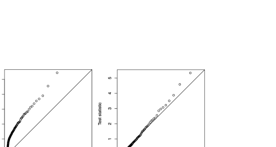
Figure 2: An example with $n=100$ and $p=10$ orthogonal predictors, and the true coefficient vector having 3 nonzero, large components. Shown are quantile–quantile plots for the drop in $\mathrm{RSS}$ test applied to forward stepwise regression at the 4th step and the covariance test for the lasso path at the 4th step.

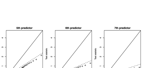
Figure 3: The same setup as in Figure 2, but here we show the covariance test at the 5th, 6th and 7th steps along the lasso path, from left to right, respectively. The solid line has slope 1, while the broken lines have slopes $1/2,1/3,1/4$, as predicted by Theorem 1.

5.1 Orthogonal predictor matrix.

Similar to our example from the start of Section 2, we generated $n=100$ observations with $p=10$ orthogonal predictors. The true coefficient vector $\beta^{*}$ contained 3 nonzero components equal to 6, and the rest zero. The error variance was $\sigma^{2}=1$, so that the truly active predictors had strong effects and always entered the model first, with both forward stepwise and the lasso. Figure 2 shows the results for testing the 4th (truly inactive) predictor to enter, averaged over 500 simulations; the left panel shows the chi-squared test (drop in $\mathrm{RSS}$) applied at the 4th step in forward stepwise regression, and the right panel shows the covariance test applied at the 4th step of the lasso path. We see that the $\operatorname{Exp}(1)$ distribution provides a good finite-sample approximation for the distribution of the covariance statistic, while $\chi^{2}_{1}$ is a poor approximation for the drop in $\mathrm{RSS}$.

Table 2: Simulation results for the first predictor to enter for a global null true model. We vary the number of predictors $p$, correlation parameter $\rho$ and structure of the predictor correlation matrix. Shown are the mean, variance and tail probability $\mathbb{P}(T_{1}>q_{0.95})$ of the covariance statistic $T_{1}$, where $q_{0.95}$ is the $95\%$ quantile of the $\operatorname{Exp}(1)$ distribution, computed over 500 simulated data sets for each setup. Standard errors are given by “se.” (The panel in the bottom left corner is missing because the equal data correlation setup is not defined for $p>n$.)

	Equal data corr			Equal pop’n corr			$\bolds{\mathit{AR}(1)}$			Block diagonal
$\bolds{\rho}$	Mean	Var	Tail pr	Mean	Var	Tail pr	Mean	Var	Tail pr	Mean	Var	Tail pr
$n=100$, $p=10$
0	0.966	1.157	0.062	1.120	1.951	0.090	1.017	1.484	0.070	1.058	1.548	0.060
0.2	0.972	1.178	0.066	1.119	1.844	0.086	1.034	1.497	0.074	1.069	1.614	0.078
0.4	0.963	1.219	0.060	1.115	1.724	0.092	1.045	1.469	0.060	1.077	1.701	0.076
0.6	0.960	1.265	0.070	1.095	1.648	0.086	1.048	1.485	0.066	1.074	1.719	0.086
0.8	0.958	1.367	0.060	1.062	1.624	0.092	1.034	1.471	0.062	1.062	1.687	0.072
se	0.007	0.015	0.001	0.010	0.049	0.001	0.013	0.043	0.001	0.010	0.047	0.001
$n=100$, $p=50$
0	0.929	1.058	0.048	1.078	1.721	0.074	1.039	1.415	0.070	0.999	1.578	0.048
0.2	0.920	1.032	0.038	1.090	1.476	0.074	0.998	1.391	0.054	1.064	2.062	0.052
0.4	0.928	1.033	0.040	1.079	1.382	0.068	0.985	1.373	0.060	1.076	2.168	0.062
0.6	0.950	1.058	0.050	1.057	1.312	0.060	0.978	1.425	0.054	1.060	2.138	0.060
0.8	0.982	1.157	0.056	1.035	1.346	0.056	0.973	1.439	0.060	1.046	2.066	0.068
se	0.010	0.030	0.001	0.011	0.037	0.001	0.009	0.041	0.001	0.011	0.103	0.001
$n=100$, $p=200$
0				1.004	1.017	0.054	1.029	1.240	0.062	0.930	1.166	0.042
0.2				0.996	1.164	0.052	1.000	1.182	0.062	0.927	1.185	0.046
0.4				1.003	1.262	0.058	0.984	1.016	0.058	0.935	1.193	0.048
0.6				1.007	1.327	0.062	0.954	1.000	0.050	0.915	1.231	0.044
0.8				0.989	1.264	0.066	0.961	1.135	0.060	0.914	1.258	0.056
se				0.008	0.039	0.001	0.009	0.028	0.001	0.007	0.032	0.001

Figure 3 shows the results for testing the 5th, 6th and 7th predictors to enter the lasso model. An $\operatorname{Exp}(1)$-based test will now be conservative: at a nominal $5\%$ level, the actual type I errors are about $1\%$, $0.2\%$ and $0.0\%$, respectively. The solid line has slope 1, and the broken lines have slopes $1/2,1/3,1/4$, as predicted by Theorem 1.

5.2 General predictor matrix.

In Table 2, we simulated null data (i.e., $\beta^{*}=0$), and examined the distribution of the covariance test statistic $T_{1}$ for the first predictor to enter. We varied the numbers of predictors $p$, correlation parameter $\rho$, and structure of the predictor correlation matrix. In the first two correlation setups, the correlation between each pair of predictors was $\rho$, in the data and population, respectively. In the $\mathit{AR}(1)$ setup, the correlation between predictors $j$ and $j^{\prime}$ is $\rho^{|j-j^{\prime}|}$. Finally, in the block diagonal setup, the correlation matrix has two equal-sized blocks, with population correlation $\rho$ in each block. We computed the mean, variance and tail probability of the covariance statistic $T_{1}$ over $500$ simulated data sets for each setup. We see that the $\operatorname{Exp}(1)$ distribution is a reasonably good approximation throughout.

In Table 3, the setup was the same as in Table 2, except that we set the first $k$ coefficients of the true coefficient vector equal to 4, and the rest zero, for $k=1,2,3$. The dimensions were also fixed at $n=100$ and $p=50$. We computed the mean, variance, and tail probability of the covariance statistic $T_{k+1}$ for entering the next (truly inactive) $(k+1)$st predictor, discarding those simulations in which a truly inactive predictor was selected in the first $k$ steps. (This occurred $1.7\%$, $4.0\%$ and $7.0\%$ of the time, resp.) Again, we see that the $\operatorname{Exp}(1)$ approximation is reasonably accurate throughout.

Table 3: Simulation results for the $(k+1)$st predictor to enter for a model with $k$ truly nonzero coefficients, across $k=1,2,3$. The rest of the setup is the same as in Table 2 except that the dimensions were fixed at $n=100$ and $p=50$. The values are conditional on the event that the $k$ truly active variables enter in the first $k$ steps

	Equal data corr			Equal pop’n corr			$\bolds{\mathit{AR}(1)}$			Block diagonal
$\bolds{\rho}$	Mean	Var	Tail pr	Mean	Var	Tail pr	Mean	Var	Tail pr	Mean	Var	Tail pr
$k=1$ and 2nd predictor to enter
0	0.933	1.091	0.048	1.105	1.628	0.078	1.023	1.146	0.064	1.039	1.579	0.060
0.2	0.940	1.051	0.046	1.039	1.554	0.082	1.017	1.175	0.060	1.062	2.015	0.062
0.4	0.952	1.126	0.056	1.016	1.548	0.084	0.984	1.230	0.056	1.042	2.137	0.066
0.6	0.938	1.129	0.064	0.997	1.518	0.079	0.964	1.247	0.056	1.018	1.798	0.068
0.8	0.818	0.945	0.039	0.815	0.958	0.044	0.914	1.172	0.062	0.822	0.966	0.037
se	0.010	0.024	0.002	0.011	0.036	0.002	0.010	0.030	0.002	0.015	0.087	0.002
$k=2$ and 3rd predictor to enter
0	0.927	1.051	0.046	1.119	1.724	0.094	0.996	1.108	0.072	1.072	1.800	0.064
0.2	0.928	1.088	0.044	1.070	1.590	0.080	0.996	1.113	0.050	1.043	2.029	0.060
0.4	0.918	1.160	0.050	1.042	1.532	0.085	1.008	1.198	0.058	1.024	2.125	0.066
0.6	0.897	1.104	0.048	0.994	1.371	0.077	1.012	1.324	0.058	0.945	1.568	0.054
0.8	0.719	0.633	0.020	0.781	0.929	0.042	1.031	1.324	0.068	0.771	0.823	0.038
se	0.011	0.034	0.002	0.014	0.049	0.003	0.009	0.022	0.002	0.013	0.073	0.002
$k=3$ and 4th predictor to enter
0	0.925	1.021	0.046	1.080	1.571	0.086	1.044	1.225	0.070	1.003	1.604	0.060
0.2	0.926	1.159	0.050	1.031	1.463	0.069	1.025	1.189	0.056	1.010	1.991	0.060
0.4	0.922	1.215	0.048	0.987	1.351	0.069	0.980	1.185	0.050	0.918	1.576	0.053
0.6	0.905	1.158	0.048	0.888	1.159	0.053	0.947	1.189	0.042	0.837	1.139	0.052
0.8	0.648	0.503	0.008	0.673	0.699	0.026	0.940	1.244	0.062	0.647	0.593	0.015
se	0.014	0.037	0.002	0.016	0.044	0.003	0.014	0.031	0.003	0.016	0.073	0.002

In Figure 4, we estimate the power curves for significance testing via the drop in RSS test for forward stepwise regression, and the covariance test for the lasso. In the former, we use simulation-derived cutpoints, and in the latter we use the theoretically-based $\operatorname{Exp}(1)$ cutpoints, to control the type I error at the 5% level. We find that the tests have similar power, though the cutpoints for forward stepwise would not be typically available in practice. For more details, see the figure caption.

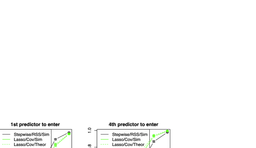
Figure 4: Estimated power curves for significance tests using forward stepwise regression and the drop in RSS statistic, as well as the lasso and the covariance statistic. The results are averaged over 1000 simulations with $n=100$ and $p=10$ predictors drawn i.i.d. from $N(0,1)$ and $\sigma^{2}=1$. On the left, there is one truly nonzero regression coefficient, and we varied its magnitude (the effect size parameter on the $x$-axis). We examined the first step of the forward stepwise and lasso procedures. On the right, in addition to a nonzero coefficient with varying effect size (on the $x$-axis), there are 3 additional large coefficients in the true model. We examined the 4th step in forward stepwise and the lasso, after the 3 strong variables have been entered. For the power curves in both panels, we use simulation-based cutpoints for forward stepwise to control the type I error at the 5% level; for the lasso we do the same, but also display the results for the theoretically-based [$\operatorname{Exp}(1)$] cutpoint. Note that in practice, simulation-based cutpoints would not typically be available.

6 The case of unknown $\sigma^{2}$.

Up until now, we have assumed that the error variance $\sigma^{2}$ is known; in practice it will typically be unknown. In this case, provided that $n>p$, we can easily estimate it and proceed by analogy to standard linear model theory. In particular, we can estimate $\sigma^{2}$ by the mean squared residual error $\hat{\sigma}^{2}=\|y-X\hat{\beta}^{\mathrm{LS}}\|_{2}^{2}/(n-p)$, with $\hat{\beta}^{\mathrm{LS}}$ being the regression coefficients from $y$ on $X$ (i.e., the full model). Plugging this estimate into the covariance statistic in (5) yields a new statistic $F_{k}$ that has an asymptotic $F$-distribution under the null:

$$F_{k}=\frac{\langle y,X\hat{\beta}(\lambda_{k+1})\rangle-\langle y,X_{A}\tilde{\beta}_{A}(\lambda_{k+1})\rangle}{\hat{\sigma}^{2}}\stackrel{{\scriptstyle d}}{{\rightarrow}}F_{2,n-p}.$$ (48)

This follows because $F_{k}=T_{k}/(\hat{\sigma}^{2}/\sigma^{2})$, the numerator $T_{k}$ being asymptotically $\operatorname{Exp}(1)=\chi_{2}^{2}/2$, the denominator $\hat{\sigma}^{2}/\sigma^{2}$ being asymptotically $\chi_{n-p}^{2}/\break(n-p)$, and we claim that the two are independent. Why? Note that the lasso solution path is unchanged if we replace $y$ by $P_{X}y$, so the lasso fitted values in $T_{k}$ are functions of $P_{X}y$; meanwhile, $\hat{\sigma}^{2}$ is a function of $(I-P_{X})y$. The quantities $P_{X}y$ and $(I-P_{X})y$ are uncorrelated, and hence independent (recalling normality of $y$), so $T_{k}$ and $\hat{\sigma}^{2}$ are functions of independent quantities and, therefore, independent.

As an example, consider one of the setups from Table 2, with $n=100$, $p=80$ and predictor correlation of the $\mathit{AR}(1)$ form $\rho^{|j-j^{\prime}|}$. The true model is null, and we test the first predictor to enter along the lasso path. (We choose $n,p$ of roughly equal sizes here to expose the differences between the $\sigma^{2}$ known and unknown cases.) Table 4 shows the results of 1000 simulations from each of the $\rho=0$ and $\rho=0.8$ scenarios. We see that with $\sigma^{2}$ estimated, the $F_{2,n-p}$ distribution provides a more accurate finite-sample approximation than does $\operatorname{Exp}(1)$.

Table 4: Comparison of $\operatorname{Exp}(1)$, $F_{2,{N-p}}$, and the observed (empirical) null distribution of the covariance statistic, when $\sigma^{2}$ has been estimated. We examined 1000 simulated data sets with $n=100$, $p=80$ and the correlation between predictors $j$ and $j^{\prime}$ equal to $\rho^{|j-j^{\prime}|}$. We are testing the first step of the lasso path, and the true model is the global null. Results are shown for $\rho=0.0$ and $0.8$. The third column shows the tail probability $\mathbb{P}(T_{1}>q_{0.95})$ computed over the 1000 simulations, where $q_{0.95}$ is the $95\%$ quantile from the appropriate distribution [either $\operatorname{Exp}(1)$ or $F_{2,n-p}$]

	Mean	Variance	95% quantile	Tail prob
$\rho=0$
Observed	1.17	2.10	3.75
$\operatorname{Exp}(1)$	1.00	1.00	2.99	0.082
$F_{2,n-p}$	1.11	1.54	3.49	0.054
$\rho=0.8$
Observed	1.14	1.70	3.77
$\operatorname{Exp}(1)$	1.00	1.00	2.99	0.097
$F_{2,n-p}$	1.11	1.54	3.49	0.064

When $p\geq n$, estimation of $\sigma^{2}$ is not nearly as straightforward; one idea is to estimate $\sigma^{2}$ from the least squares fit on the support of the model selected by cross-validation. One would then hope that the resulting statistic, with this plug-in estimate of $\sigma^{2}$, is close in distribution to $F_{2,n-r}$ under the null, where $r$ is the size of the model chosen by cross-validation. This is by analogy to the low-dimensional $n>p$ case in (48), but is not supported by rigorous theory. Simulations (withheld for brevity) show that this approximation is not too far off, but that the variance of the observed statistic is sometimes inflated compared that of an $F_{2,n-r}$ distribution (this unaccounted variability is likely due to the model selection process via cross-validation). Other authors have argued that using cross-validation to estimate $\sigma^{2}$ when $p\gg n$ is not necessarily a good approach, as it can be anti-conservative; see, for example, Fan, Guo and Hao (2012), Sun and Zhang (2012) for alternative techniques. In future work, we will address the important issue of estimating $\sigma^{2}$ in the context of the covariance statistic, when $p\geq n$.

7 Real data examples.

We demonstrate the use of covariance test with some real data examples. As mentioned previously, in any serious application of significance testing over many variables (many steps of the lasso path), we would need to consider the issue of multiple comparisons, which we do not here. This is a topic for future work.

7.1 Wine data.

Table 5 shows the results for the wine quality data taken from the UCI database. There are $p=11$ predictors, and $n=1599$ observations, which we split randomly into approximately equal-sized training and test sets. The outcome is a wine quality rating, on a scale between 0 and 10. The table shows the training set $p$-values from forward stepwise regression (with the chi-squared test) and the lasso (with the covariance test). Forward stepwise enters 6 predictors at the 0.05 level, while the lasso enters only 3.

Table 5: Wine data: forward stepwise and lasso $p$-values. The values are rounded to 3 decimal places. For the lasso, we only show $p$-values for the steps in which a predictor entered the model and stayed in the model for the remainder of the path (i.e., if a predictor entered the model at a step but then later left, we do not show this step—we only show the step corresponding to its last entry point)

Forward stepwise				Lasso
Step	Predictor	RSS test	$\bolds{p}$-value	Step	Predictor	Cov test	$\bolds{p}$-value
1	Alcohol	$315.216$	0.000	$1$	Alcohol	$79.388$	0.000
2	Volatile_acidity	$137.412$	0.000	$2$	Volatile_acidity	$77.956$	0.000
3	Sulphates	$18.571$	0.000	$3$	Sulphates	$10.085$	0.000
4	Chlorides	$10.607$	0.001	$4$	Chlorides	$1.757$	0.173
5	pH	$4.400$	0.036	$5$	Total_sulfur_dioxide	$0.622$	0.537
6	Total_sulfur_dioxide	$3.392$	0.066	$6$	pH	$2.590$	0.076
7	Residual_sugar	$0.607$	0.436	$7$	Residual_sugar	$0.318$	0.728
8	Citric_acid	$0.878$	0.349	$8$	Citric_acid	$0.516$	0.597
9	Density	$0.288$	0.592	$9$	Density	$0.184$	0.832
10	Fixed_acidity	$0.116$	0.733	$10$	Free_sulfur_dioxide	$0.000$	1.000
11	Free_sulfur_dioxide	$0.000$	0.997	$11$	Fixed_acidity	$0.114$	0.892

In the left panel of Figure 5, we repeated this $p$-value computation over 500 random splits into training test sets. The right panel shows the corresponding test set prediction error for the models of each size. The lasso test error decreases sharply once the 3rd predictor is added, but then somewhat flattens out from the 4th predictor onward; this is in general qualitative agreement with the lasso $p$-values in the left panel, the first 3 being very small, and the 4th $p$-value being about 0.2. This also echoes the well-known difference between hypothesis testing and minimizing prediction error. For example, the $C_{p}$ statistic stops entering variables when the $p$-value is larger than about 0.16.

Figure 5: Wine data: the data were randomly divided 500 times into roughly equal-sized training and test sets. The left panel shows the training set $p$-values for forward stepwise regression and the lasso. The right panel show the test set error for the corresponding models of each size.

Figure 6: HIV data: the data were randomly divided 50 times into training and test sets of size 150 and 907, respectively. The left panel shows the training set $p$-values for forward stepwise regression and the lasso. The right panel shows the test set error for the corresponding models of each size.

7.2 HIV data.

Rhee et al. (2003) study six nucleotide reverse transcriptase inhibitors (NRTIs) that are used to treat HIV-1. The target of these drugs can become resistant through mutation, and they compare a collection of models for predicting the (log) susceptibility of the drugs, a measure of drug resistance, based on the location of mutations. We focused on the first drug (3TC), for which there are $p=217$ sites and $n=1057$ samples. To examine the behavior of the covariance test in the $p>n$ setting, we divided the data at random into training and test sets of size 150 and 907, respectively, a total of 50 times. Figure 6 shows the results, in the same format as Figure 5. We used the model chosen by cross-validation to estimate $\sigma^{2}$. The covariance test for the lasso suggests that there are only one or two important predictors (in marked contrast to the chi-squared test for forward stepwise), and this is confirmed by the test error plot in the right panel.

8 Extensions.

We discuss some extensions of the covariance statistic, beyond significance testing for the lasso. The proposals here are supported by simulations [in terms of having an $\operatorname{Exp}(1)$ null distribution], but we do not offer any theory. This may be a direction for future work.

8.1 The elastic net.

The elastic net estimate [Zou and Hastie (2005)] is defined as

$$\hat{\beta}^{\mathrm{en}}=\mathop{\operatorname{argmin}}_{\beta\in\mathbb{R}^{p}}\frac{1}{2}\|y-X\beta\|_{2}^{2}+\lambda\|\beta\|_{1}+\frac{\gamma}{2}\|\beta\|_{2}^{2},$$ (49)

where $\gamma\geq 0$ is a second tuning parameter. It is not hard to see that this can actually be cast as a lasso estimate with predictor matrix $\widetilde{X}=\bigl{[}{{\begin{array}[]{c}X\\ \sqrt{\gamma}I\end{array}}}\bigr{]}\in\mathbb{R}^{(n+p)\times p}$ and outcome $\tilde{y}=(y,0)\in\mathbb{R}^{n+p}$. This shows that, for a fixed $\gamma$, the elastic net solution path is piecewise linear over $\lambda$, with each knot marking the entry (or deletion) of a variable from the active set. We therefore define the covariance statistic in the same manner as we did for the lasso; fixing $\gamma$, to test the predictor entering at the $k$th step (knot $\lambda_{k}$) in the elastic net path, we consider the statistic

$$T_{k}=\bigl{(}\bigl{\langle}y,X\hat{\beta}^{\mathrm{en}}(\lambda_{k+1},\gamma)\bigr{\rangle}-\bigl{\langle}y,X_{A}\tilde{\beta}_{A}^{\mathrm{en}}(\lambda_{k+1},\gamma)\bigr{\rangle}\bigr{)}/\sigma^{2},$$

where as before, $\lambda_{k+1}$ is next knot in the path, $A$ is the active set of predictors just before $\lambda_{k}$ and $\tilde{\beta}^{\mathrm{en}}_{A}$ is the elastic net solution using only the predictors $X_{A}$. The precise expression for the elastic net solution in (49), for a given active set and signs, is the same as it is for the lasso (see Section 2.3), but with $(X_{A}^{T}X_{A})^{-1}$ replaced by $(X_{A}^{T}X_{A}+\gamma I)^{-1}$. This generally creates a complication for the theory in Sections 3 and 4. But in the orthogonal $X$ case, we have $(X_{A}^{T}X_{A}+\gamma I)^{-1}=I/(1+\gamma)$ and so

$$T_{k}=1/(1+\gamma)\cdot|U_{(k)}|\bigl{(}|U_{(k)}|-|U_{(k+1)}|\bigr{)}/\sigma^{2}$$

with $U_{j}=X_{j}^{T}y$, $j=1,\ldots,p$. This means that for an orthogonal $X$, under the null,

$$(1+\gamma)\cdot T_{k}\stackrel{{\scriptstyle d}}{{\rightarrow}}\operatorname{Exp}(1)$$

and one is tempted to use this approximation beyond the orthogonal setting as well. In Figure 7, we evaluated the distribution of $(1+\gamma)T_{1}$ (for the first predictor to enter), for orthogonal and correlated scenarios, and for three different values of $\gamma$. Here, $n=100$, $p=10$ and the true model was null. It seems to be reasonably close to $\operatorname{Exp}(1)$ in all cases.

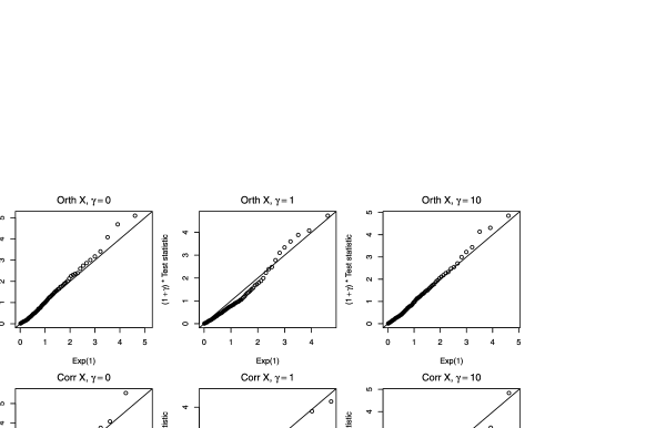
Figure 7: Elastic net: an example with $n=100$ and $p=10$, for orthogonal and correlated predictors (having pairwise population correlation 0.5), and three different values of the ridge penalty parameter $\gamma$.

8.2 Generalized linear models and the Cox model.

Consider the estimate from an $\ell_{1}$-penalized generalized linear model:

$$\hat{\beta}^{\mathrm{glm}}=\mathop{\operatorname{argmin}}_{\beta\in\mathbb{R}^{p}}-\sum_{i=1}^{n}\log f(y_{i};x_{i},\beta)+\lambda\|\beta\|_{1},$$ (50)

where $f(y_{i};x_{i},\beta)$ is an exponential family density, a function of the predictor measurements $x_{i}\in\mathbb{R}^{p}$ and parameter $\beta\in\mathbb{R}^{p}$. Note that the usual lasso estimate in (2) is a special case of this form when $f$ is the Gaussian density with known variance $\sigma^{2}$. The natural parameter in (50) is $\eta_{i}=x_{i}^{T}\beta$, for $i=1,\ldots,n$, related to the mean of $y_{i}$ via a link function $g(\mathbb{E}[y_{i}|x_{i}])=\eta_{i}$.

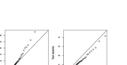
Figure 8: Lasso logistic regression: an example with $n=100$ and $p=10$ predictors, i.i.d. from $N(0,1)$. In the left panel, all true coefficients are zero; on the right, the first coefficient is large, and the rest are zero. Shown are quantile–quantile plots of the covariance test statistic (at the first and second steps, resp.), generated over 500 data sets, versus its conjectured asymptotic distribution, $\operatorname{Exp}(1)$.

Having solved (50) with $\lambda=0$ (i.e., this is simply maximum likelihood), producing a vector of fitted values $\hat{\eta}=X\hat{\beta}^{\mathrm{glm}}\in\mathbb{R}^{n}$, we might define degrees of freedom as

$$\operatorname{df}(\hat{\eta})=\sum_{i=1}^{n}\operatorname{Cov}(y_{i},\hat{\eta}_{i}).$$ (51)

This is the implicit concept used by Efron (1986) in his definition of the “optimism” of the training error. The same idea could be used to define degrees of freedom for the penalized estimate in (50) for any $\lambda>0$, and this motivates the definition of the covariance statistic, as follows. If the tuning parameter value $\lambda=\lambda_{k}$ marks the entry of a new predictor into the active set $A$, then we define the covariance statistic

$$T_{k}=\bigl{\langle}y,X\hat{\beta}^{\mathrm{glm}}(\lambda_{k+1})\bigr{\rangle}-\bigl{\langle}y,X_{A}\tilde{\beta}_{A}^{\mathrm{glm}}(\lambda_{k+1})\bigr{\rangle},$$ (52)

where $\lambda_{k+1}$ is the next value of the tuning parameter at which the model changes (a variable enters or leaves the active set), and $\tilde{\beta}_{A}^{\mathrm{glm}}$ is the estimate from the penalized generalized linear model (50) using only predictors in $A$. Unlike in the Gaussian case, the solution path in (50) is not generally piecewise linear over $\lambda$, and there is not an algorithm to deliver the exact the values of $\lambda$ at which variables enter the model (we still refer to these as knots in the path). However, one can numerically approximate these knot values; for example, see Park and Hastie (2007). By analogy to the Gaussian case, we would hope that $T_{k}$ has an asymptotic $\operatorname{Exp}(1)$ distribution under the null. Though we have not rigorously investigated this conjecture, simulations seem to support it.

As example, consider the logistic regression model for binary data. Now $\eta_{i}=\log(\mu_{i}/(1-\mu_{i}))$, with $\mu_{i}=\mathbb{P}(y_{i}=1|x_{i})$. Figure 8 shows the simulation results from comparing the null distribution of the covariance test statistic in (52) to $\operatorname{Exp}(1)$. Here, we used the glmpath package in R [Park and Hastie (2007)] to compute an approximate solution path and locations of knots. The null distribution of the test statistic looks fairly close to $\operatorname{Exp}(1)$.

For general likelihood-based regression problems, let $\eta=X\beta$ and $\ell(\eta)$ denote the log likelihood. We can view maximum likelihood estimation as an iteratively weighted least squares procedure using the outcome variable

$$z(\eta)=\eta+I_{\eta}^{-1}S_{\eta},$$ (53)

where $S_{\eta}=\nabla\ell(\eta)$, and $I_{\eta}=\nabla^{2}\ell(\eta)$. This applies, for example, to the class of generalized linear models and Cox’s proportional hazards model. For the general $\ell_{1}$-penalized estimator

$$\hat{\beta}^{\mathrm{lik}}=\mathop{\operatorname{argmin}}_{\beta\in\mathbb{R}^{p}}-\ell(X\beta)+\lambda\|\beta\|_{1},$$ (54)

we can analogously define the covariance test statistic at a knot $\lambda_{k}$, marking the entry of a predictor into the active set $A$, as

$$T_{k}=\bigl{(}\bigl{\langle}I_{0}^{-1/2}S_{0},X\hat{\beta}^{\mathrm{lik}}(\lambda_{k+1})\bigr{\rangle}-\bigl{\langle}I_{0}^{-1/2}S_{0},X_{A}\tilde{\beta}^{\mathrm{lik}}_{A}(\lambda_{k+1})\bigr{\rangle}\bigr{)}/2$$ (55)

with $\lambda_{k+1}$ being the next knot in the path (at which a variable is added or deleted from the active set), and $\tilde{\beta}_{A}^{\mathrm{lik}}$ the solution of the general penalized likelihood problem (54) with predictor matrix $X_{A}$. For the binomial model, the statistic (55) reduces to expression (52). In Figure 9, we computed this statistic for Cox’s proportional hazards model, using a similar setup to that in Figure 8. The $\operatorname{Exp}(1)$ approximation for its null distribution looks reasonably accurate.

Figure 9: Lasso Cox model estimate: the basic setup is the same as in Figure 8 ($n$, $p$, the distribution of the predictors $X$, the true coefficient vector—on the left, entirely zero, and on the right, one large coefficient). Shown are quantile–quantile plots of the covariance test statistic (at the first and second steps, resp.), generated over 500 data sets, versus the $\operatorname{Exp}(1)$ distribution.

9 Discussion.

We proposed a simple covariance statistic for testing the significance of predictor variables as they enter the active set, along the lasso solution path. We showed that the distribution of this statistic is asymptotically $\operatorname{Exp}(1)$, under the null hypothesis that all truly active predictors are contained in the current active set. [See Theorems 1, 2 and 3; the conditions required for this convergence result vary depending on the step $k$ along the path that we are considering, and the covariance structure of the predictor matrix $X$; the $\operatorname{Exp}(1)$ limiting distribution is in some cases a conservative upper bound under the null.] Such a result accounts for the adaptive nature of the lasso procedure, which is not true for the usual chi-squared test (or $F$-test) applied to, for example, forward stepwise regression.

We feel that our work has shed light not only on the lasso path (as given by LARS), but also, at a high level, on forward stepwise regression. Both the lasso and forward stepwise start by entering the predictor variable most correlated with the outcome (thinking of standardized predictors), but the two differ in what they do next. Forward stepwise is greedy, and once it enters this first variable, it proceeds to fit the first coefficient fully, ignoring the effects of other predictors. The lasso, on the other hand, increases (or decreases) the coefficient of the first variable only as long as its correlation with the residual is larger than that of the inactive predictors. Subsequent steps follow similarly. Intuitively, it seems that forward stepwise regression inflates coefficients unfairly, while the lasso takes more appropriately sized steps. This intuition is confirmed in one sense by looking at degrees of freedom (recall Section 2.4). The covariance test and its simple asymptotic null distribution reveal another way in which the step sizes used by the lasso are “just right.”

The problem of assessing significance in an adaptive linear model fit by the lasso is a difficult one, and what we have presented in this paper by no means a complete solution. We describe some current work and ideas for future projects below.

• Significance test for generic lasso models. A natural direction to consider is the generic lasso testing problem: given a lasso model computed at some fixed value of $\lambda$, how do we carry out a significance test for each predictor in the active set? Work on this is in progress.

• Nonasymptotic null distributions. A geometric characterization of the first knot in the lasso path provides an alternative test for the global null hypothesis, $\beta^{*}=0$. When all predictors have unit norm, $\|X_{i}\|_{2}=1$, for $i=1,\ldots,p$, this test has the form

  $$\frac{1-\Phi(\lambda_{1}/\sigma)}{1-\Phi(\lambda_{2}/\sigma)}\sim\operatorname{Unif}(0,1).$$

  Remarkably, this above result is exact (nonasymptotic), valid for any $n$ and $p$, requiring (essentially) only Gaussianity of the errors, and no real assumptions about the matrix $X$. For most reasonably behaved predictor matrices $X$, the $\operatorname{Exp}(1)$ approximation agrees closely with this test. Details are in Taylor, Loftus and Tibshirani (2013). Work to extend this formula to subsequent steps along the solution path, that is, to test a hypothesis beyond the global null, is underway.

• Generalizations to other penalties and models. The manuscript of Taylor, Loftus and Tibshirani (2013) applies to a regularized regression setting with a general seminorm penalty, and derives explicit results for the group lasso and nuclear norm penalties (in addition to the lasso penalty). The nuclear norm result yields a test for principal components and matrix completion. The recent work of Grazier G’Sell, Taylor and Tibshirani (2013) studies the covariance test for graphical models, based on a sparse estimate of the inverse covariance matrix.

• Sequential procedures with false discovery rate control. It is also interesting to consider how the sequence of covariance test $p$-values can be used to construct a sequential test with good power properties, and a guaranteed bound on its false discovery rate. A number of such approaches are proposed in Grazier G’Sell et al. (2013).

• Proper $p$-values for forward stepwise. Perhaps surprisingly, a test analogous to the covariance test can be used in forward stepwise regression, to construct valid $p$-values for this greedy procedure. This work is in progress.

• Other related problems include: estimation of $\sigma^{2}$ when $p\geq n$, in the context of the covariance test; power calculations and confidence interval estimation; theory for linear models having strong and weak signals (large and small true coefficients); theory for the elastic net, generalized linear models, and the Cox model.

As is clear from the above discussion, the covariance test work has created much excitement and activity among our close collaborators and students. It is our hope that the current paper will also broadly stimulate other researchers’ interest in this area, and that at some point, the joint efforts of the community will yield a full set of inferential tools for the lasso and other commonly used adaptive procedures.

Appendix

.1 Proof of Lemma 1.

By continuity of the lasso solution path at $\lambda_{k}$,

$$P_{A}y-\lambda_{k}\bigl{(}X_{A}^{T}\bigr{)}^{+}s_{A}=P_{A\cup\{j\}}y-\lambda_{k}\bigl{(}X_{A\cup\{j\}}^{T}\bigr{)}^{+}s_{A\cup\{j\}}$$

and, therefore,

$$(P_{A\cup\{j\}}-P_{A})y=\lambda_{k}\bigl{(}\bigl{(}X_{A\cup\{j\}}^{T}\bigr{)}^{+}s_{A\cup\{j\}}-\bigl{(}X_{A}^{T}\bigr{)}^{+}s_{A}\bigr{)}.$$ (56)

From this, we can obtain two identities: the first is

$$y^{T}(P_{A\cup\{j\}}-P_{A})y=\lambda_{k}^{2}\cdot\bigl{\|}\bigl{(}X_{A\cup\{j\}}^{T}\bigr{)}^{+}s_{A\cup\{j\}}-\bigl{(}X_{A}^{T}\bigr{)}^{+}s_{A}\bigr{\|}_{2}^{2},$$ (57)

obtained by squaring both sides in (56) (more precisely, taking the inner product of the left-hand side with itself and the right-hand side with itself), and noting that $(P_{A\cup\{j\}}-P_{A})^{2}=P_{A\cup\{j\}}-P_{A}$; the second is

$$y^{T}\bigl{(}\bigl{(}X_{A\cup\{j\}}^{T}\bigr{)}^{+}s_{A\cup\{j\}}-\bigl{(}X_{A}^{T}\bigr{)}^{+}s_{A}\bigr{)}$$

(58)

$$\qquad=\lambda_{k}\cdot\bigl{\|}\bigl{(}X_{A\cup\{j\}}^{T}\bigr{)}^{+}s_{A\cup\{j\}}-\bigl{(}X_{A}^{T}\bigr{)}^{+}s_{A}\bigr{\|}_{2}^{2},$$

obtained by taking the inner product of both sides in (56) with $y$, and then using (57). Plugging (57) and (.1) in for the first and second terms in (2.3), respectively, then gives the result in (9).

.2 Proof of Lemma 4.

Note that

$$g(j_{1},s_{1})>g(j,s)$$

$$\qquad\Longleftrightarrow\quad\frac{g(j_{1},s_{1})-ss_{1}R_{j,j_{1}}g(j_{1},s_{1})}{1-ss_{1}R_{j,j_{1}}}>\frac{g(j,s)-ss_{1}R_{j,j_{1}}g(j_{1},s_{1})}{1-ss_{1}R_{j,j_{1}}}$$

$$\qquad\Longleftrightarrow\quad g(j_{1},s_{1})>h^{(j_{1},s_{1})}(j,s),$$

the first step following since $1-ss_{1}R_{j,j_{1}}>0$, and the second step following from the definition of $h^{(j_{1},s_{1})}$. The intersection of the right-hand side above, over all $(j,s)\neq(j_{1},s_{1})$, is equivalent to

$$g(j_{1},s_{1})>g(j_{1},-s_{1}),\qquad g(j_{1},s_{1})>M(j_{1},s_{1}).$$

But the former inequality is the same as $g(j_{1},s_{1})>0$, because $g(j_{1},s_{1})$ and $g(j_{1},-s_{1})$ have opposite signs. Further, the inequality $g(j_{1},s_{1})>0$ is redundant, as $M(j_{1},s_{1})\geq 0$. This gives the result.

.3 Proof of Lemma 5.

By l’Hôpital’s rule,

$$\lim_{m\rightarrow\infty}\frac{\overline{\Phi}(u(t,m))}{\overline{\Phi}(m)}=\lim_{m\rightarrow\infty}\frac{\phi(u(t,m))}{\phi(m)}\cdot\frac{\partial u(t,m)}{\partial m},$$

where $\phi$ is the standard normal density. First, note that

$$\frac{\partial(t,m)}{\partial m}=\frac{1}{2}+\frac{m}{2\sqrt{m^{2}+4t}}\rightarrow 1\qquad\mbox{as }m\rightarrow\infty.$$

Also, a straightforward calculation shows

$$\log{\phi\bigl{(}u(t,m)\bigr{)}}-\log{\phi(m)}=\frac{m^{2}}{2}\bigl{(}1-\sqrt{1+4t/m^{2}}\bigr{)}-\frac{t}{2}\rightarrow-t\qquad\mbox{as }m\rightarrow\infty,$$

where in the last step we used the fact that $(1-\sqrt{1+4t/m^{2}})/(2/m^{2})\rightarrow-t/2$, again by l’Hôpital’s rule. Therefore, $\phi(u(t,m))/\phi(m)\rightarrow e^{-t}$, which completes the proof.

.4 Proof of Lemma 6.

Fix $\varepsilon>0$, and choose $m_{0}$ large enough that

$$\biggl{|}\frac{\overline{\Phi}(u(t,m/\sigma))}{\overline{\Phi}(m/\sigma)}-e^{-t}\biggr{|}\leq\varepsilon\qquad\mbox{for all }m\geq m_{0}.$$

Starting from (4.1),

$$\bigl{|}\mathbb{P}(T_{1}>t)-e^{-t}\bigr{|} \leq \sum_{j_{1},s_{1}}\int_{0}^{\infty}\biggl{|}\frac{\overline{\Phi}(u(t,m/\sigma))}{\overline{\Phi}(m/\sigma)}-e^{-t}\biggr{|}\overline{\Phi}(m/\sigma)F_{M(j_{1},s_{1})}(dm)$$

$$\leq \varepsilon\sum_{j_{1},s_{1}}\int_{m_{0}}^{\infty}\overline{\Phi}(m/\sigma)F_{M(j_{1},s_{1})}(dm)+\sum_{j_{1},s_{1}}\int_{0}^{m_{0}}F_{M(j_{1},s_{1})}(dm)$$

$$\leq \varepsilon\sum_{j_{1},s_{1}}\mathbb{P}\bigl{(}g(j_{1},s_{1})>M(j_{1},s_{1})\bigr{)}+\sum_{j_{1},s_{1}}\mathbb{P}\bigl{(}M(j_{1},s_{1})\leq m_{0}\bigr{)}.$$

Above, the term multiplying $\varepsilon$ is equal to 1, and the second term can be made arbitrarily small (say, less than $\varepsilon$) by taking $p$ sufficiently large.

.5 Proof of Theorem 2.

We will show that for any fixed $m_{0}>0$ and $j_{1},s_{1}$,

$$\mathbb{P}\bigl{(}M(j_{1},s_{1})\leq m_{0}\bigr{)}\leq c^{|S|},$$ (59)

where $S\subseteq\{1,\ldots,p\}\setminus\{j_{1}\}$ is as in the theorem for $j=j_{1}$, with size $|S|\geq d_{p}$, and $c<1$ is a constant (not depending on $j_{1}$). This would imply that

$$\sum_{j_{1},s_{1}}\mathbb{P}\bigl{(}M(j_{1},s_{1})\leq m_{0}\bigr{)}\leq 2p\cdot c^{d_{p}}\rightarrow 0\qquad\mbox{as }p\rightarrow\infty,$$

where we used the fact that $d_{p}/\log{p}\rightarrow\infty$ by (27). The above sum tending to zero now implies the desired convergence result by Lemma 6, and hence it suffices to show (59). To this end, consider

$$M(j_{1},s_{1}) = \max_{j\neq j_{1},s}\frac{sU_{j}-sR_{j,j_{1}}U_{j_{1}}}{1-ss_{1}R_{j,j_{1}}}$$

$$\geq \max_{j\neq j_{1}}\frac{|U_{j}-R_{j,j_{1}}U_{j_{1}}|}{1+|R_{j,j_{1}}|}$$

$$\geq \max_{j\in S}\frac{|U_{j}-R_{j,j_{1}}U_{j_{1}}|}{2},$$

where in both inequalities above we used the fact that $|R_{j,j_{1}}|<1$. We can therefore use the bound

$$\mathbb{P}\bigl{(}M(j_{1},s_{1})\leq m_{0}\bigr{)}\leq\mathbb{P}\bigl{(}|V_{j}|\leq m_{0},j\in S\bigr{)},$$

where we define $V_{j}=(U_{j}-R_{j,j_{1}}U_{j_{1}})/2$ for $j\in S$. Let $r=|S|$, and without a loss of generality, let $S=\{1,\ldots,r\}$. We will show that

$$\mathbb{P}\bigl{(}|V_{1}|\leq m_{0},\ldots,|V_{r}|\leq m_{0}\bigr{)}\leq c^{r}$$ (60)

for $c=\Phi(2m_{0}/(\sigma\delta))-\Phi(-2m_{0}/(\sigma\delta))<1$, by induction; this would complete the proof, as it would imply (59). Before presenting this argument, we note a few important facts. First, the condition in (26) is really a statement about conditional variances:

$$\operatorname{Var}\bigl{(}U_{i}|U_{\ell},\ell\in S\setminus\{i\}\bigr{)}=\sigma^{2}\cdot\bigl{[}1-R_{i,S\setminus\{i\}}(R_{S\setminus\{i\},S\setminus\{i\}})^{-1}R_{S\setminus\{i\},i}\bigr{]}\geq\sigma^{2}\delta^{2}$$

$$\eqntext{\mbox{for all }i\in S,}$$ (61)

where recall that $U_{j}=X_{j}^{T}y$, $j=1,\ldots,p$. Second, since $U_{1},\ldots,U_{r}$ are jointly normal, we have

$$\operatorname{Var}\bigl{(}U_{i}|U_{\ell},\ell\in S^{\prime}\bigr{)}\geq\operatorname{Var}\bigl{(}U_{i}|U_{\ell},\ell\in S\setminus\{i\}\bigr{)}\geq\sigma^{2}\delta^{2}$$

(62)

$$\eqntext{\displaystyle\mbox{for any }S^{\prime}\subseteq S\setminus\{i\}\mbox{ and }i\in S,}$$ (63)

which can be verified using the conditional variance formula (i.e., the law of total variance). Finally, the collection $V_{1},\ldots,V_{r}$ is independent of $U_{j_{1}}$, because these random variables are jointly normal, and $\mathbb{E}[V_{j}U_{j_{1}}]=0$ for all $j=1,\ldots,r$.

Now we give the inductive argument for (60). For the base case, note that $V_{1}\sim N(0,\tau_{1}^{2})$, where its variance is

$$\tau_{1}^{2}=\operatorname{Var}(V_{1})=\operatorname{Var}(V_{1}|U_{j_{1}})=\operatorname{Var}(U_{1})/4\geq\sigma^{2}\delta^{2}/4,$$

the second equality is due to the independence of $V_{1}$ and $U_{j_{1}}$, and the last inequality comes from the fact that conditioning can only decrease the variance, as stated above in (.5). Hence,

$$\mathbb{P}\bigl{(}|V_{1}|\leq m_{0}\bigr{)} = \Phi(m_{0}/\tau_{1})-\Phi(-m_{0}/\tau_{1})$$

$$\leq \Phi\bigl{(}2m_{0}/(\sigma\delta)\bigr{)}-\Phi\bigl{(}-2m_{0}/(\sigma\delta)\bigr{)}=c.$$

Assume as the inductive hypothesis that $\mathbb{P}(|V_{1}|\leq m_{0},\ldots,|V_{q}|\leq m_{0})\leq c^{q}$. Then

$$\mathbb{P}\bigl{(}|V_{1}|\leq m_{0},\ldots,|V_{q+1}|\leq m_{0}\bigr{)}$$

$$\qquad=\mathbb{P}\bigl{(}|V_{q+1}|\leq m_{0}||V_{1}|\leq m_{0},\ldots,|V_{q}|\leq m_{0}\bigr{)}\cdot c^{q}.$$

We have, using the independence of $V_{1},\ldots,V_{q+1}$ and $U_{j_{1}}$,

$$V_{q+1}|V_{1},\ldots,V_{q} \stackrel{{\scriptstyle d}}{{=}} V_{q+1}|V_{1},\ldots,V_{q},U_{j_{1}}$$

$$\stackrel{{\scriptstyle d}}{{=}} V_{q+1}|U_{1},\ldots,U_{q},U_{j_{1}}$$

$$\stackrel{{\scriptstyle d}}{{=}} N\bigl{(}0,\tau_{q+1}^{2}\bigr{)},$$

where the variance is

$$\tau_{q+1}^{2}=\operatorname{Var}(V_{q+1}|U_{1},\ldots,U_{q},U_{j_{1}})=\operatorname{Var}(U_{q+1}|U_{1},\ldots,U_{q})/4\geq\sigma^{2}\delta^{2}/4$$

and here we again used the fact that conditioning further can only reduce the variance, as in (.5). Therefore,

$$\mathbb{P}\bigl{(}|V_{q+1}|\leq m_{0}|V_{1},\ldots,V_{q}\bigr{)}\leq\Phi\bigl{(}2m_{0}/(\sigma\delta)\bigr{)}-\Phi\bigl{(}-2m_{0}/(\sigma\delta)\bigr{)}=c$$

and so

$$\mathbb{P}\bigl{(}|V_{1}|\leq m_{0},\ldots,|V_{q+1}|\leq m_{0}\bigr{)}\leq c\cdot c^{q}=c^{q+1},$$

completing the inductive step.

.6 Proof of Lemma 7.

Notice that

$$g(j_{k},s_{k})>g(j,s)$$

$$\qquad\Longleftrightarrow\quad g(j_{k},s_{k})(1-\Sigma_{j,j^{\prime}}/\Sigma_{jj})>g(j,s)-(\Sigma_{j,j^{\prime}}/\Sigma_{jj})g(j_{k},s_{k}).$$

We now handle division by $1-\Sigma_{j,j^{\prime}}/\Sigma_{jj}$ in three cases:

• if $1-\Sigma_{j,j^{\prime}}/\Sigma_{jj}>0$, then

  $$g(j_{k},s_{k})>g(j,s)\quad\Longleftrightarrow\quad g(j_{k},s_{k})>\frac{g(j,s)-(\Sigma_{j,j^{\prime}}/\Sigma_{jj})g(j_{k},s_{k})}{1-\Sigma_{j,j^{\prime}}/\Sigma_{jj}};$$

• if $1-\Sigma_{j,j^{\prime}}/\Sigma_{jj}<0$, then

  $$g(j_{k},s_{k})>g(j,s)\quad\Longleftrightarrow\quad g(j_{k},s_{k})<\frac{g(j,s)-(\Sigma_{j,j^{\prime}}/\Sigma_{jj})g(j_{k},s_{k})}{1-\Sigma_{j,j^{\prime}}/\Sigma_{jj}};$$

• if $1-\Sigma_{j,j^{\prime}}/\Sigma_{jj}=0$, then

  $$g(j_{k},s_{k})>g(j,s)\quad\Longleftrightarrow\quad 0>g(j,s)-(\Sigma_{j,j^{\prime}}/\Sigma_{jj})g(j_{k},s_{k}).$$

Using this breakdown, we see that the statement $g(j_{k},s_{k})>g(j,s)$ for all $(j,s)\neq(j_{k},s_{k})$ is then equivalent to

$$g(j_{k},s_{k}) > g(j_{k},-s_{k}),\qquad g(j_{k},s_{k})>M^{+}(j_{k},s_{k}),$$

$$g(j_{k},s_{k}) < M^{-}(j_{k},s_{k}),\qquad 0>M^{0}(j_{k},s_{k}).$$

Noting that $g(j_{k},s_{k})$ and $g(j_{k},-s_{k})$ must have opposite signs, the above is equivalent to

$$g(j_{k},s_{k}) > 0,\qquad g(j_{k},s_{k})>M^{+}(j_{k},s_{k}),$$

$$g(j_{k},s_{k}) < M^{-}(j_{k},s_{k}),\qquad 0>M^{0}(j_{k},s_{k}),$$

which gives the result in the lemma.

.7 Proof of Lemma 8.

Define $\sigma_{k}=\sigma/\sqrt{C(j_{k},s_{k})}$ and $u(a,b)=(b+\sqrt{b^{2}+4a})/2$. Exactly as before (dropping for simplicity the notational dependence of $g,M^{+}$ on $j_{k},s_{k}$),

$$g\bigl{(}g-M^{+}\bigr{)}/\sigma_{k}^{2}>t,\qquad g>M^{+}\quad\Longleftrightarrow\quad g/\sigma_{k}>u\bigl{(}t,M^{+}/\sigma_{k}\bigr{)}.$$

Therefore, we can rewrite (4.2) as

$$\mathbb{P}(\widetilde{T}_{k}>t) = \sum_{j_{k},s_{k}}\mathbb{P}\bigl{(}g(j_{k},s_{k})/\sigma_{k}>u\bigl{(}t,M^{+}(j_{k},s_{k})/\sigma_{k}\bigr{)},$$

$$\hskip 29.0ptg(j_{k},s_{k})<M^{-}(j_{k},s_{k}),0>M^{0}(j_{k},s_{k})\bigr{)}.$$

Note that we have dropped the inequality $g(j_{k},s_{k})>0$ from each term, as it is implied by the first inequality $g(j_{k},s_{k})/\sigma_{k}>u(t,M^{+}(j_{k},s_{k})/\sigma_{k})\geq 0$. We can upper bound the right-hand side above by replacing $g(j_{k},s_{k})<M^{-}(j_{k},s_{k})$ with

$$g(j_{k},s_{k})<M^{-}(j_{k},s_{k})+u\bigl{(}t\sigma_{k}^{2},M^{+}(j_{k},s_{k})\bigr{)}-M^{+}(j_{k},s_{k}),$$

because $u(a,b)\geq b$ for all $a\geq 0$ and $b$. Furthermore, Lemma 10 (Appendix .10) shows that indeed $\sigma_{k}^{2}=\sigma^{2}/C(j_{k},s_{k})=\operatorname{Var}(g(j_{k},s_{k}))$ for fixed $j_{k},s_{k}$, and hence $g(j_{k},s_{k})/\sigma_{k}$ is standard normal for fixed $j_{k},s_{k}$. Therefore,

$$\mathbb{P}(\widetilde{T}_{k}>t) \leq \sum_{j_{k},s_{k}}\int\bigl{[}\Phi\bigl{(}m^{-}/\sigma_{k}+u\bigl{(}t,m^{+}/\sigma_{k}\bigr{)}-m^{+}/\sigma_{k}\bigr{)}-\Phi\bigl{(}u\bigl{(}t,m^{+}/\sigma_{k}\bigr{)}\bigr{)}\bigr{]}$$

$$\hskip 26.0pt{}\times G_{j_{k},s_{k}}\bigl{(}dm^{+},dm^{-},dm^{0}\bigr{)},$$

where

$$G_{j_{k},s_{k}}\bigl{(}dm^{+},dm^{-},dm^{0}\bigr{)}$$

$$\qquad=1\bigl{\{}m^{+}<m^{-},m^{0}<0\bigr{\}}\cdot F_{M^{+}(j_{k},s_{k}),M^{-}(j_{k},s_{k}),M^{0}(j_{k},s_{k})}\bigl{(}dm^{+},dm^{-},dm^{0}\bigr{)}$$

with $F_{M^{+}(j_{k},s_{k}),M^{-}(j_{k},s_{k}),M^{0}(j_{k},s_{k})}$ the joint distribution of $M^{+}(j_{k},s_{k})$,$M^{-}(j_{k},s_{k})$, $M^{0}(j_{k},s_{k})$, and we used the fact that $g$ is independent of $M^{+},\break M^{-},M^{0}$ for fixed $j_{k},s_{k}$. From (.7),

$$\mathbb{P}(\widetilde{T}_{k}>t)-e^{-t}$$

$$\qquad\leq\sum_{j_{k},s_{k}}\int\biggl{(}\frac{\Phi(m^{-}/\sigma_{k}+u(t,m^{+}/\sigma_{k})-m^{+}/\sigma_{k})-\Phi(u(t,m^{+}/\sigma_{k}))}{\Phi(m^{-}/\sigma_{k})-\Phi(m^{+}/\sigma_{k})}-e^{-t}\biggr{)}$$ (65)

$$\hskip 59.0pt{}\times\bigl{[}\Phi\bigl{(}m^{-}/\sigma_{k}\bigr{)}-\Phi\bigl{(}m^{+}/\sigma_{k}\bigr{)}\bigr{]}\cdot G_{j_{k},s_{k}}\bigl{(}dm^{+},dm^{-},dm^{0}\bigr{)},$$

where we here used the fact that

$$\sum_{j_{k},s_{k}}\int\bigl{[}\Phi\bigl{(}m^{-}/\sigma_{k}\bigr{)}-\Phi\bigl{(}m^{+}/\sigma_{k}\bigr{)}\bigr{]}G_{j_{k},s_{k}}\bigl{(}dm^{+},dm^{-},dm^{0}\bigr{)}$$

$$\qquad=\sum_{j_{k},s_{k}}\mathbb{P}\bigl{(}g(j_{k},s_{k})>M^{+}(j_{k},s_{k}),g(j_{k},s_{k})<M^{-}(j_{k},s_{k}),0>M^{0}(j_{k},s_{k})\bigr{)}$$

$$\qquad\geq\sum_{j_{k},s_{k}}\mathbb{P}\bigl{(}g(j_{k},s_{k})>0,g(j_{k},s_{k})>M^{+}(j_{k},s_{k}),$$

$$\hskip 63.0ptg(j_{k},s_{k})<M^{-}(j_{k},s_{k}),0>M^{0}(j_{k},s_{k})\bigr{)}$$

$$\qquad=1,$$

the last equality following by Lemma 7 (i.e., each term in the last sum is exactly the probability of $j_{k},s_{k}$ maximizing $g$). We show in Lemma 11 (Appendix .11) that

$$\lim_{m^{+}\rightarrow\infty}\frac{\Phi(m^{-}+u(t,m^{+})-m^{+})-\Phi(u(t,m^{+}))}{\Phi(m^{-})-\Phi(m^{+})}\leq e^{-t},$$

provided that $m^{-}>m^{+}$. Hence, fix $\varepsilon>0$, and choose $m_{0}$ sufficiently large, so that for each $k$,

$$\frac{\Phi(m^{-}/\sigma_{k}+u(t,m^{+}/\sigma_{k})-m^{+}/\sigma_{k})-\Phi(u(t,m^{+}/\sigma_{k}))}{\Phi(m^{-}/\sigma_{k})-\Phi(m^{+}/\sigma_{k})}-e^{-t}\leq\varepsilon$$

$$\eqntext{\displaystyle\mbox{for all }m^{-}/\sigma_{k}>m^{+}/\sigma_{k}\geq m_{0}.}$$ (66)

Working from (.7),

$$\mathbb{P}(\widetilde{T}_{k}>t)-e^{-t}$$

$$\qquad\leq\varepsilon\sum_{j_{k},s_{k}}\int_{m^{+}/\sigma_{k}\geq m_{0}}\bigl{[}\Phi\bigl{(}m^{-}/\sigma_{k}\bigr{)}-\Phi\bigl{(}m^{+}/\sigma_{k}\bigr{)}\bigr{]}G_{j_{k},s_{k}}\bigl{(}dm^{+},dm^{-},dm^{0}\bigr{)}$$

$$\quad\qquad{}+\sum_{j_{k},s_{k}}\int_{m^{+}/\sigma_{k}\leq m_{0}}G_{j_{k},s_{k}}\bigl{(}dm^{+},dm^{-},dm^{0}\bigr{)}.$$

Note that the first term on the right-hand side above is $\leq\varepsilon$, and the second term is bounded by $\sum_{j_{k},s_{k}}\mathbb{P}(M^{+}(j_{k},s_{k})\leq m_{0}\sigma_{k})$, which by assumption can be made arbitrarily small (smaller than, say, $\varepsilon$) by taking $p$ large enough.

.8 Proof of Lemma 9.

For now, we reintroduce the notational dependence of the process $g$ on $A,s_{A}$, as this will be important. We show in Lemma 12 (Appendix .12) that for any fixed $j_{k},s_{k},j,s$,

$$\frac{g^{(A,s_{A})}(j,s)-(\Sigma_{j_{k},j}/\Sigma_{j_{k},j_{k}})g^{(A,s_{A})}(j_{k},s_{k})}{1-\Sigma_{j_{k},j}/\Sigma_{j_{k},j_{k}}}=g^{(A\cup\{j_{k}\},s_{A\cup\{j_{k}\}})}(j,s),$$

where $\Sigma_{j_{k},j}=\mathbb{E}[g^{(A,s_{A})}(j_{k},s_{k}),g^{(A,s_{A})}(j,s)]$, as given in (30), and as usual, $s_{A\cup\{j_{k}\}}$ denotes the concatenation of $s_{A}$ and $s_{k}$. According to its definition in (LABEL:eqmp), therefore,

$$M^{+}(j_{k},s_{k})=\max_{(j,s)\in S^{+}(j_{k},s_{k})}g^{(A\cup\{j_{k}\},s_{A\cup\{j_{k}\}})}(j,s)$$

and hence on the event $E(j_{k},s_{k})$, since we have $g^{(A,s_{A})}(j_{k},s_{k})>M^{+}(j_{k},s_{k})$,

$$M^{+}(j_{k},s_{k})$$

$$\quad=\max_{(j,s)\in S^{+}(j_{k},s_{k})}g^{(A\cup\{j_{k}\},s_{A\cup\{j_{k}\}})}(j,s)$$

$$\qquad\hskip 54.0pt{}\times 1\bigl{\{}g^{(A\cup\{j_{k}\},s_{A\cup\{j_{k}\}})}(j,s)<g^{(A,s_{A})}(j_{k},s_{k})\bigr{\}}$$

$$\quad\leq\max_{j\notin A\cup\{j_{k}\},s}g^{(A\cup\{j_{k}\},s_{A\cup\{j_{k}\}})}(j,s)\cdot 1\bigl{\{}g^{(A\cup\{j_{k}\},s_{A\cup\{j_{k}\}})}(j,s)<g^{(A,s_{A})}(j_{k},s_{k})\bigr{\}}$$

$$\quad=M(j_{k},s_{k}).$$

This means that (now we return to writing $g^{(A,s_{A})}$ as $g$, for brevity)

$$\sum_{j_{k},s_{k}}\mathbb{P}\bigl{(}\bigl{\{}C(j_{k},s_{k})\cdot g(j_{k},s_{k})\bigl{(}g(j_{k},s_{k})-M(j_{k},s_{k})\bigr{)}/\sigma^{2}>t\bigr{\}}\cap E(j_{k},s_{k})\bigr{)}$$

$$\quad\leq\sum_{j_{k},s_{k}}\mathbb{P}\bigl{(}\bigl{\{}C(j_{k},s_{k})\cdot g(j_{k},s_{k})\bigl{(}g(j_{k},s_{k})-M^{+}(j_{k},s_{k})\bigr{)}/\sigma^{2}>t\bigr{\}}\cap E(j_{k},s_{k})\bigr{)}$$

and so $\lim_{p\rightarrow\infty}\mathbb{P}(T_{k}>t)\leq\lim_{p\rightarrow\infty}\mathbb{P}(\widetilde{T}_{k}>t)\leq e^{-t}$, the desired conclusion.

.9 Proof of Theorem 3.

Since we are assuming that $\mathbb{P}(B)\rightarrow 1$, we know that $\mathbb{P}(T_{k}>t|B)-\mathbb{P}(T_{k}>t)\rightarrow 0$, so we only need to consider the marginal limiting distribution of $T_{k}$. We write $A=A_{0}$ and $s_{A}=s_{A_{0}}$. The general idea here is similar to that used in the proof of Theorem 2. Fixing $m_{0}$ and $j_{k},s_{k}$, we will show that

$$\mathbb{P}\bigl{(}M^{+}(j_{k},s_{k})\leq m_{0}\sigma_{k}\bigr{)}\leq c^{|S|},$$ (67)

where $S\subseteq\{1,\ldots,p\}\setminus(A\cup\{j_{k}\})$ is as in the statement of the theorem for $j=j_{k}$, with size $|S|\geq d_{p}$, and $c<1$ is a constant (not depending on $j_{k}$). Also, as in the proof of Lemma 8, we abbreviated $\sigma_{k}=\sigma/\sqrt{C(j_{k},s_{k})}$. This bound would imply that

$$\sum_{j_{k},s_{k}}\mathbb{P}\bigl{(}M^{+}(j_{k},s_{k})\leq m_{0}\sigma_{k}\bigr{)}\leq 2p\cdot c^{d_{p}}\rightarrow 0\qquad\mbox{as }p\rightarrow\infty,$$

since $d_{p}/\log{p}\rightarrow 0$. The above sum converging to zero is precisely the condition required by Lemma 9, which then gives the desired (conservative) exponential limit for $T_{k}$. Hence, it is suffices to show (67). For this, we start by recalling the definition of $M^{+}$ in (LABEL:eqmp):

$$M^{+}(j_{k},s_{k})=\max_{(j,s)\in S^{+}(j_{k},s_{k})}\frac{g(j,s)-(\Sigma_{j_{k},j}/\Sigma_{j_{k},j_{k}})g(j_{k},s_{k})}{1-\Sigma_{j_{k},j}/\Sigma_{j_{k},j_{k}}}$$

$$\eqntext{\displaystyle\mbox{where }S^{+}(j_{k},s_{k})=\biggl{\{}(j,s)\dvtx j\notin A\cup\{j_{k}\},\frac{\Sigma_{j_{k},j}}{\Sigma_{j_{k},j_{k}}}<1\biggr{\}}.}$$ (68)

Here, we write $\Sigma_{j_{k},j}=\mathbb{E}[g(j_{k},s_{k})g(j,s)]$; note that $\Sigma_{j_{k},j_{k}}=\sigma^{2}_{k}$ (as shown in Lemma 10). First, we show that the conditions of the theorem actually imply that $S^{+}(j_{k},s_{k})\supseteq S\times\{-1,1\}^{|S|}$. This is true because for $j\in S$ and any $s\in\{-1,1\}$, we have $|R_{j,j_{k}}|/R_{j_{k},j_{k}}<\eta/(2-\eta)$ by (45), and

$$|R_{j,j_{k}}|/R_{j_{k},j_{k}}<\eta/(2-\eta) \quad\Longrightarrow\quad \biggl{|}\frac{R_{j,j_{k}}}{R_{j_{k},j_{k}}}\cdot\frac{s_{k}-X_{j_{k}}^{T}(X_{A}^{T})^{+}s_{A}}{s-X_{j}^{T}(X_{A}^{T})^{+}s_{A}}\biggr{|}<1$$

$$\quad\Longrightarrow\quad \Sigma_{j_{k},j}/\Sigma_{j_{k},j_{k}}<1.$$

The first implication uses the assumption (43), as $|s_{k}-X_{j_{k}}^{T}(X_{A}^{T})^{+}s_{A}|\leq 1+\|(X_{A})^{+}X_{j_{k}}\|_{1}\leq 2-\eta$ and $|s-X_{j}^{T}(X_{A}^{T})^{+}s_{A}|\geq 1-\|(X_{A})^{+}X_{j_{k}}\|_{1}\geq\eta$, and the second simply follows from the definition of $\Sigma_{j_{k},j}$ and $\Sigma_{j_{k},j_{k}}$. Therefore,

$$M^{+}(j_{k},s_{k})\geq\max_{j\in S,s}\frac{g(j,s)-(\Sigma_{j_{k},j}/\Sigma_{j_{k},j_{k}})g(j_{k},s_{k})}{1-\Sigma_{j_{k},j}/\Sigma_{j_{k},j_{k}}}.$$

Let $U_{j}=X_{j}^{T}(I-P_{A})y$ and $\theta_{j_{k},j}=R_{j_{k},j}/R_{j_{k},j_{k}}$ for $j\in S$. By the arguments given in the proof of Lemma 12, we can rewrite the right-hand side above, yielding

$$M^{+}(j_{k},s_{k}) \geq \max_{j\in S,s}\frac{U_{j}-\theta_{j_{k},j}U_{j_{k}}}{s-X_{j}^{T}(X_{A\cup\{j_{k}\}}^{T})^{+}s_{A\cup\{j_{k}\}}}$$

$$= \max_{j\in S,s}\frac{s(U_{j}-\theta_{j_{k},j}U_{j_{k}})}{1-sX_{j}^{T}(X_{A\cup\{j_{k}\}}^{T})^{+}s_{A\cup\{j_{k}\}}}$$

$$\geq \max_{j\in S}\frac{|U_{j}-\theta_{j_{k},j}U_{j_{k}}|}{1+|X_{j}^{T}(X_{A\cup\{j_{k}\}}^{T})^{+}s_{A\cup\{j_{k}\}}|}$$

$$\geq \max_{j\in S}\frac{|U_{j}-\theta_{j_{k},j}U_{j_{k}}|}{2},$$

where the last two inequalities above follow as $|X_{j}^{T}(X_{A\cup\{j_{k}\}})^{+}s_{A\cup\{j_{k}\}}|\,{<}\,1$ for all $j\in S$, which itself follows from the assumption that $\|(X_{A\cup\{j_{k}\}})^{+}X_{j}\|_{\infty}<1$ for all $j\in S$, in (46). Hence,

$$\mathbb{P}\bigl{(}M^{+}(j_{k},s_{k})\leq m_{0}\sigma_{k}\bigr{)}\leq\mathbb{P}\bigl{(}|V_{j}|\leq m_{0}\sigma_{k},j\in S\bigr{)},$$

where $V_{j}=(U_{j}-\theta_{j_{k},j}U_{j_{k}})/2$. Writing without a loss of generality $r=|S|$ and $S=\{1,\ldots,r\}$, it now remains to show that

$$\mathbb{P}\bigl{(}|V_{1}|\leq m_{0}\sigma_{k},\ldots,|V_{r}|\leq m_{0}\sigma_{k}\bigr{)}\leq c^{r}.$$ (69)

Similar to the arguments in the proof of Theorem 2, we will show (69) by induction, for the constant $c=\Phi(2m_{0}\sqrt{C}/(\delta\eta))-\Phi(-2m_{0}\sqrt{C}/(\delta\eta))<1$. Before this, it is helpful to discuss three important facts. First, we note that (44) is actually a lower bound on the ratio of conditional to unconditional variances:

$$\operatorname{Var}\bigl{(}U_{i}|U_{\ell},\ell\in S\setminus\{i\}\bigr{)}/\operatorname{Var}(U_{i})$$

$$\qquad=\bigl{[}R_{ii}-R_{i,S\setminus\{i\}}(R_{S\setminus\{i\},S\setminus\{i\}})^{-1}R_{S\setminus\{i\},i}\bigr{]}/R_{ii}\geq\delta^{2}\qquad\mbox{for all }i\in S.$$

Second, conditioning on a smaller set of variables can only increase the conditional variance:

$$\operatorname{Var}\bigl{(}U_{i}|U_{\ell},\ell\in S^{\prime}\bigr{)}\geq\operatorname{Var}\bigl{(}U_{i}|U_{\ell},\ell\in S\setminus\{i\}\bigr{)}\geq\delta^{2}\sigma^{2}R_{ii}$$

$$\eqntext{\displaystyle\mbox{for any }S^{\prime}\subseteq S\setminus\{i\}\mbox{ and }i\in S,}$$ (70)

which holds as $U_{1},\ldots,U_{r}$ are jointly normal. Third, and lastly, the collection $V_{1},\ldots,V_{r}$ is independent of $U_{j_{k}}$, since these variables are all jointly normal, and it is easily verified that $\mathbb{E}[V_{j}U_{j_{k}}]=0$ for each $j=1,\ldots,r$.

We give the inductive argument for (69). For the base case, we have $V_{1}\sim N(0,\tau_{1}^{2})$, where

$$\tau_{1}^{2}=\operatorname{Var}(V_{1})=\operatorname{Var}(V_{1}|U_{j_{k}})=\operatorname{Var}(U_{1})/4\geq\delta^{2}\sigma^{2}R_{11}/4.$$

Above, in the second equality, we used that $V_{1}$ and $U_{j_{k}}$ are independent, and in the last inequality, that conditioning on fewer variables (here, none) only increases the variance. This means that

$$\mathbb{P}\bigl{(}|V_{1}|\leq m_{0}\sigma_{k}\bigr{)}\leq\mathbb{P}\bigl{(}|Z|\leq 2m_{0}\sigma_{k}/(\delta\sigma\sqrt{R_{11}})\bigr{)}\leq\mathbb{P}\bigl{(}|Z|\leq 2m_{0}\sqrt{C}/(\delta\eta)\bigr{)}=c,$$

where $Z$ is standard normal; note that in the last inequality above, we applied the upper bound

$$\frac{\sigma^{2}_{k}}{\sigma^{2}R_{11}}=\frac{\Sigma_{j_{k},j_{k}}}{\sigma^{2}R_{11}}=\frac{R_{j_{k},j_{k}}}{R_{11}}\cdot\frac{1}{[s_{k}-X_{j_{k}}^{T}(X_{A}^{T})^{+}s_{A}]^{2}}\leq\frac{C}{\eta^{2}}.$$

Now, for the inductive hypothesis, assume that $\mathbb{P}(|V_{1}|\leq m_{0}\sigma_{k},\ldots,|V_{q}|\leq m_{0}\sigma_{k})\leq c^{q}$. Consider

$$\mathbb{P}\bigl{(}|V_{1}|\leq m_{0}\sigma_{k},\ldots,|V_{q+1}|\leq m_{0}\sigma_{k}\bigr{)}$$

$$\qquad=\mathbb{P}\bigl{(}|V_{q+1}|\leq m_{0}\sigma_{k}||V_{1}|\leq m_{0}\sigma_{k},\ldots,|V_{q}|\leq m_{0}\sigma_{k}\bigr{)}\cdot c^{q}.$$

Using the independence of $V_{1},\ldots,V_{q+1}$ and $U_{j_{k}}$,

$$V_{q+1}|V_{1},\ldots,V_{q} \stackrel{{\scriptstyle d}}{{=}} V_{q+1}|V_{1},\ldots,V_{q},U_{j_{k}}$$

$$\stackrel{{\scriptstyle d}}{{=}} V_{q+1}|U_{1},\ldots,U_{q},U_{j_{k}}$$

$$\stackrel{{\scriptstyle d}}{{=}} N\bigl{(}0,\tau_{q+1}^{2}\bigr{)}.$$

The variance $\tau_{q+1}^{2}$ is

$$\tau_{q+1}^{2} = \operatorname{Var}(V_{q+1}|U_{1},\ldots,U_{q},U_{j_{k}})$$

$$= \operatorname{Var}(U_{q+1}|U_{1},\ldots,U_{q})/4$$

$$\geq \delta^{2}\sigma^{2}R_{q+1,q+1}/4,$$

where we again used the fact that conditioning on a smaller set of variables only makes the variance larger. Finally,

$$\mathbb{P}\bigl{(}|V_{q+1}|\leq m_{0}\sigma_{k}|V_{1},\ldots,V_{q}\bigr{)} \leq \mathbb{P}\bigl{(}|Z|\leq 2m_{0}\sigma_{k}/(\delta\sigma\sqrt{R_{q+1,q+1}})\bigr{)}$$

$$\leq \mathbb{P}\bigl{(}|Z|\leq 2m_{0}\sqrt{C}/(\delta\eta)\bigr{)}$$

$$= c,$$

where we used $\sigma_{k}^{2}/(\sigma^{2}R_{q+1,q+1})\leq C/\eta^{2}$ as above, and so

$$\mathbb{P}\bigl{(}|V_{1}|\leq m_{0}\sigma_{k},\ldots,|V_{q+1}|\leq m_{0}\sigma_{k}\bigr{)}\leq c\cdot c^{q}=c^{q+1}.$$

This completes the inductive proof.

.10 Statement and proof of Lemma 10.

Lemma 10

For any fixed $A,s_{A}$, and any $j\notin A$, $s\in\{-1,1\}$, we have

$$\operatorname{Var}\bigl{(}g(j,s)\bigr{)}=\frac{X_{j}^{T}(I-P_{A})X_{j}^{T}\sigma^{2}}{[s-X_{j}^{T}(X_{A}^{T})^{+}s_{A}]^{2}}=\frac{\sigma^{2}}{\|(X_{A\cup\{j\}}^{T})^{+}s_{A\cup\{j\}}-(X_{A}^{T})^{+}s_{A}\|_{2}^{2}},$$

where $s_{A\cup\{j\}}$ denotes the concatenation of $s_{A}$ and $s$.

We will show that

$$\frac{[s-X_{j}^{T}(X_{A}^{T})^{+}s_{A}]^{2}}{X_{j}^{T}(I-P_{A})X_{j}^{T}}=\bigl{\|}\bigl{(}X_{A\cup\{j\}}^{T}\bigr{)}^{+}s_{A\cup\{j\}}-\bigl{(}X_{A}^{T}\bigr{)}^{+}s_{A}\bigr{\|}_{2}^{2}.$$ (71)

The right-hand side above, after a straightforward calculation, is shown to be equal to

$$s_{A\cup\{j\}}^{T}\bigl{(}X_{A\cup\{j\}}^{T}X_{A\cup\{j\}}\bigr{)}^{-1}s_{A\cup\{j\}}-s_{A}\bigl{(}X_{A}^{T}X_{A}\bigr{)}^{-1}s_{A}.$$ (72)

Now let $z=(X_{A\cup\{j\}}^{T}X_{A\cup\{j\}})^{-1}s_{A\cup\{j\}}$. In block form,

$$\left[\matrix{X_{A}^{T}X_{A}&X_{A}^{T}X_{j}\vspace*{5pt}\cr X_{j}^{T}X_{A}&X_{j}^{T}X_{j}}\right]\left[\matrix{z_{1}\cr z_{2}}\right]=\left[\matrix{s_{A}\cr s}\right].$$ (73)

Solving for $z_{1}$ in the first row yields

$$z_{1}=\bigl{(}X_{A}^{T}X_{A}\bigr{)}^{-1}s_{A}-(X_{A})^{+}X_{j}z_{2}$$

and, therefore, (72) is equal to

$$s_{A}^{T}z_{1}+sz_{2}-s_{A}^{T}\bigl{(}X_{A}^{T}X_{A}\bigr{)}^{-1}s_{A}=\bigl{[}s-s_{A}^{T}(X_{A})^{+}X_{j}\bigr{]}z_{2}.$$ (74)

Solving for $z_{2}$ in the second row of (73) gives

$$z_{2}=\frac{s-s_{A}^{T}(X_{A})^{+}X_{j}}{X_{j}^{T}(I-P_{A})X_{j}}.$$

Plugging this value into (74) produces the left-hand side in (71), completing the proof.

.11 Statement and proof of Lemma 11.

Lemma 11

If $v=v(m)$ satisfies $v>m$, then for any $t\geq 0$,

$$\lim_{m\rightarrow\infty}\frac{\Phi(v+u(t,m)-m)-\Phi(u(t,m))}{\Phi(v)-\Phi(m)}\leq e^{-t}.$$

First note, using a Taylor series expansion of $\sqrt{1+4t/m^{3}}$, that for sufficiently large $m$,

$$u(t,m)\geq m+\frac{t}{m}-\frac{t^{2}}{m^{3}}.$$ (75)

Also, a simple calculation shows that $\partial(u(t,m)-m)/\partial m\leq 0$ for all $m$, so that

$$u(t,w)-w\leq u(t,m)-m\qquad\mbox{for all }w\geq m.$$ (76)

Now consider

$$\Phi\bigl{(}v+u(t,m)-m\bigr{)}-\Phi\bigl{(}u(t,m)\bigr{)} = \int_{u(t,m)}^{v+u(t,m)-m}\frac{e^{-z^{2}/2}}{\sqrt{2\pi}}\,dz$$

$$= \int_{m}^{v}\frac{e^{-(w+u(t,m)-m)^{2}/2}}{\sqrt{2\pi}}\,dw$$

$$\leq \int_{m}^{v}\frac{e^{-u(t,m)^{2}/2}}{\sqrt{2\pi}}\,dw$$

$$\leq \int_{m}^{v}\frac{e^{-(w+t/m-t^{2}/m^{3})^{2}/2}}{\sqrt{2\pi}}\,dw,$$

where the first inequality follows from (76), and the second from (75) (assuming $m$ is large enough). Continuing from the last upper bound,

$$\int_{m}^{v}\frac{e^{-(w+t/m-t^{2}/m^{3})^{2}/2}}{\sqrt{2\pi}}\,dw=e^{-t}\int_{m}^{v}\frac{e^{-w^{2}/2}}{\sqrt{2\pi}}f(w,t)\,dw,$$

where

$$f(w,t)=\exp\biggl{(}\frac{t^{2}}{2w^{2}}+\frac{t^{3}}{w^{4}}-\frac{t^{4}}{2w^{6}}\biggr{)}.$$

Therefore, we have

$$\frac{\Phi(v+u(t,m)-m)-\Phi(u(t,m))}{\Phi(v)-\Phi(m)}-e^{-t}$$

(77)

$$\qquad\leq\biggl{(}\frac{\int_{m}^{v}(e^{-w^{2}/2}/\sqrt{2\pi})f(w,t)\,dw}{\int_{m}^{v}(e^{-w^{2}/2}/\sqrt{2\pi})\,dw}-1\biggr{)}\cdot e^{-t}.$$

It is clear that $f(w,t)\rightarrow 1$ as $w\rightarrow\infty$. Fixing $\varepsilon$, choose $m_{0}$ large enough so that for all $w\geq m_{0}$, we have $|f(w,t)-1|\leq\varepsilon$. Then the term multiplying $e^{-t}$ on the right-hand side in (.11), for $m\geq m_{0}$, is

$$\frac{\int_{m}^{v}({e^{-w^{2}/2}}/{\sqrt{2\pi}})f(w,t)\,dw}{\int_{m}^{v}(e^{-w^{2}/2}/\sqrt{2\pi})\,dw}-1\leq\frac{\int_{m}^{v}({e^{-w^{2}/2}}/{\sqrt{2\pi}})|f(w,t)-1|\,dw}{\int_{m}^{v}(e^{-w^{2}/2}/\sqrt{2\pi})\,dw}\leq\varepsilon,$$

which shows that the right-hand side in (.11) is $\leq\varepsilon\cdot e^{-t}\leq\varepsilon$, and completes the proof.

.12 Statement and proof of Lemma 12.

Lemma 12

For any fixed $j_{k},s_{k},j,s$ (and fixed $A,s_{A})$, we have

$$\qquad\frac{g^{(A,s_{A})}(j,s)-(\Sigma_{j_{k},j}/\Sigma_{j_{k},j_{k}})g^{(A,s_{A})}(j_{k},s_{k})}{1-\Sigma_{j_{k},j}/\Sigma_{j_{k},j_{k}}}=g^{(A\cup\{j_{k}\},s_{A\cup\{j_{k}\}})}(j,s),$$ (78)

where $\Sigma_{j_{k},j}$ denotes the covariance between $g^{(A,s_{A})}(j_{k},s_{k})$ and $g^{(A,s_{A})}(j,s)$,

$$\Sigma_{j_{k},j}=\frac{X_{j_{k}}^{T}(I-P_{A})X_{j}\sigma^{2}}{[s_{k}-s_{A}^{T}(X_{A})^{+}X_{j_{k}}][s-s_{A}^{T}(X_{A})^{+}X_{j}]}.$$

Simple manipulations of the left-hand side in (78) yield the expression

$$\frac{X_{j}^{T}(I-P_{A})y-\theta_{j_{k},j}\cdot X_{j_{k}}^{T}(I-P_{A})y}{s-s_{A}^{T}(X_{A})^{+}X_{j}-\theta_{j_{k},j}\cdot[s_{k}-s_{A}^{T}(X_{A})^{+}X_{j_{k}}]},$$ (79)

where $\theta_{j_{k},j}=X_{j_{k}}^{T}(I-P_{A})X_{j}/(X_{j_{k}}^{T}(I-P_{A})X_{j_{k}})$. Now it remains to show that (79) is equal to

$$\frac{X_{j}^{T}(I-P_{A\cup\{j_{k}\}})y}{s-s_{A\cup\{j_{k}\}}^{T}(X_{A\cup\{j_{k}\}})^{+}X_{j}}.$$ (80)

We show individually that the numerators and denominators in (79) and (80) are equal. First the denominators: starting with (79), notice that

$$s-s_{A}^{T}(X_{A})^{+}X_{j}-\theta_{j_{k},j}\bigl{[}s_{k}-s_{A}^{T}(X_{A})^{+}X_{j_{k}}\bigr{]}$$

$$\qquad=s-s_{A\cup\{j_{k}\}}^{T}\left[\matrix{(X_{A})^{+}(X_{j}-\theta_{j_{k},j}X_{j_{k}})\vspace*{3pt}\cr\theta_{j_{k},j}}\right].$$

By the well-known formula for partial regression coefficients,

$$\theta_{j_{k},j}=\frac{X_{j_{k}}^{T}(I-P_{A})X_{j}}{X_{j_{k}}^{T}(I-P_{A})X_{j_{k}}}=\bigl{[}(X_{A\cup\{j_{k}\}})^{+}X_{j}\bigr{]}_{j_{k}},$$

that is, $\theta_{j_{k},j}$ is the $(j_{k})$th coefficient in the regression of $X_{j}$ on $X_{A\cup\{j_{k}\}}$. Hence, to show that (.12) is equal to the denominator in (80), we need to show that $(X_{A})^{+}(X_{j}-\theta_{j_{k},j}X_{j_{k}})$ gives the coefficients in $A$ in the regression of $X_{j}$ on $X_{A\cup\{j_{k}\}}$. This follows by simply noting that the coefficients $(X_{A\cup\{j_{k}\}})^{+}X_{j}=(\theta_{A,j},\theta_{j_{k},j})$ satisfy the equation

$$X_{A}\theta_{A,j}+X_{j_{k}}\theta_{j_{k},j}=P_{A\cup\{j_{k}\}}X_{j}$$

and so solving for $\theta_{A,j}$,

$$\theta_{A,j}=(X_{A})^{+}(P_{A\cup\{j_{k}\}}X_{j}-\theta_{j_{k},j}X_{j_{k}})=(X_{A})^{+}(X_{j}-\theta_{j_{k},j}X_{j_{k}}).$$

Now for the numerators: again beginning with (79), its numerator is

$$y^{T}(I-P_{A})(X_{j}-\theta_{j_{k},j}X_{j_{k}})$$ (82)

and by essentially the same argument as above, we have

$$P_{A}(X_{j}-\theta_{j_{k},j}X_{j_{k}})=P_{A\cup\{j_{k}\}}X_{j},$$

therefore, (82) matches the numerator in (80).

References

• Beck and Teboulle (2009) {barticle}[mr] \bauthor\bsnmBeck, \bfnmAmir\binitsA. and \bauthor\bsnmTeboulle, \bfnmMarc\binitsM. (\byear2009). \btitleA fast iterative shrinkage-thresholding algorithm for linear inverse problems. \bjournalSIAM J. Imaging Sci. \bvolume2 \bpages183–202. \biddoi=10.1137/080716542, issn=1936-4954, mr=2486527 \bptokimsref\endbibitem
• Becker, Bobin and Candès (2011) {barticle}[mr] \bauthor\bsnmBecker, \bfnmStephen\binitsS., \bauthor\bsnmBobin, \bfnmJérôme\binitsJ. and \bauthor\bsnmCandès, \bfnmEmmanuel J.\binitsE. J. (\byear2011). \btitleNESTA: A fast and accurate first-order method for sparse recovery. \bjournalSIAM J. Imaging Sci. \bvolume4 \bpages1–39. \biddoi=10.1137/090756855, issn=1936-4954, mr=2765668 \bptokimsref\endbibitem
• Becker, Candès and Grant (2011) {barticle}[mr] \bauthor\bsnmBecker, \bfnmStephen R.\binitsS. R., \bauthor\bsnmCandès, \bfnmEmmanuel J.\binitsE. J. and \bauthor\bsnmGrant, \bfnmMichael C.\binitsM. C. (\byear2011). \btitleTemplates for convex cone problems with applications to sparse signal recovery. \bjournalMath. Program. Comput. \bvolume3 \bpages165–218. \biddoi=10.1007/s12532-011-0029-5, issn=1867-2949, mr=2833262 \bptokimsref\endbibitem
• Boyd et al. (2011) {barticle}[auto:STB—2014/02/12—14:17:21] \bauthor\bsnmBoyd, \bfnmS.\binitsS., \bauthor\bsnmParikh, \bfnmN.\binitsN., \bauthor\bsnmChu, \bfnmE.\binitsE., \bauthor\bsnmPeleato, \bfnmB.\binitsB. and \bauthor\bsnmEckstein, \bfnmJ.\binitsJ. (\byear2011). \btitleDistributed optimization and statistical learning via the alternative direction method of multipliers. \bjournalFaund. Trends Mach. Learn. \bvolume3 \bpages1–122. \bptokimsref\endbibitem
• Bühlmann (2013) {barticle}[mr] \bauthor\bsnmBühlmann, \bfnmPeter\binitsP. (\byear2013). \btitleStatistical significance in high-dimensional linear models. \bjournalBernoulli \bvolume19 \bpages1212–1242. \biddoi=10.3150/12-BEJSP11, issn=1350-7265, mr=3102549 \bptnotecheck year \bptokimsref\endbibitem
• Candès and Plan (2009) {barticle}[mr] \bauthor\bsnmCandès, \bfnmEmmanuel J.\binitsE. J. and \bauthor\bsnmPlan, \bfnmYaniv\binitsY. (\byear2009). \btitleNear-ideal model selection by $\ell_{1}$ minimization. \bjournalAnn. Statist. \bvolume37 \bpages2145–2177. \biddoi=10.1214/08-AOS653, issn=0090-5364, mr=2543688 \bptokimsref\endbibitem
• Candes and Tao (2006) {barticle}[mr] \bauthor\bsnmCandes, \bfnmEmmanuel J.\binitsE. J. and \bauthor\bsnmTao, \bfnmTerence\binitsT. (\byear2006). \btitleNear-optimal signal recovery from random projections: Universal encoding strategies? \bjournalIEEE Trans. Inform. Theory \bvolume52 \bpages5406–5425. \biddoi=10.1109/TIT.2006.885507, issn=0018-9448, mr=2300700 \bptokimsref\endbibitem
• Chen, Donoho and Saunders (1998) {barticle}[mr] \bauthor\bsnmChen, \bfnmScott Shaobing\binitsS. S., \bauthor\bsnmDonoho, \bfnmDavid L.\binitsD. L. and \bauthor\bsnmSaunders, \bfnmMichael A.\binitsM. A. (\byear1998). \btitleAtomic decomposition by basis pursuit. \bjournalSIAM J. Sci. Comput. \bvolume20 \bpages33–61. \biddoi=10.1137/S1064827596304010, issn=1064-8275, mr=1639094 \bptokimsref\endbibitem
• de Haan and Ferreira (2006) {bbook}[mr] \bauthor\bparticlede \bsnmHaan, \bfnmLaurens\binitsL. and \bauthor\bsnmFerreira, \bfnmAna\binitsA. (\byear2006). \btitleExtreme Value Theory: An Introduction. \bpublisherSpringer, \blocationNew York. \bidmr=2234156 \bptokimsref\endbibitem
• Donoho (2006) {barticle}[mr] \bauthor\bsnmDonoho, \bfnmDavid L.\binitsD. L. (\byear2006). \btitleCompressed sensing. \bjournalIEEE Trans. Inform. Theory \bvolume52 \bpages1289–1306. \biddoi=10.1109/TIT.2006.871582, issn=0018-9448, mr=2241189 \bptokimsref\endbibitem
• Efron (1986) {barticle}[mr] \bauthor\bsnmEfron, \bfnmBradley\binitsB. (\byear1986). \btitleHow biased is the apparent error rate of a prediction rule? \bjournalJ. Amer. Statist. Assoc. \bvolume81 \bpages461–470. \bidissn=0162-1459, mr=0845884 \bptokimsref\endbibitem
• Efron et al. (2004) {barticle}[mr] \bauthor\bsnmEfron, \bfnmBradley\binitsB., \bauthor\bsnmHastie, \bfnmTrevor\binitsT., \bauthor\bsnmJohnstone, \bfnmIain\binitsI. and \bauthor\bsnmTibshirani, \bfnmRobert\binitsR. (\byear2004). \btitleLeast angle regression. \bjournalAnn. Statist. \bvolume32 \bpages407–499. \biddoi=10.1214/009053604000000067, issn=0090-5364, mr=2060166 \bptnotecheck related \bptokimsref\endbibitem
• Fan, Guo and Hao (2012) {barticle}[mr] \bauthor\bsnmFan, \bfnmJianqing\binitsJ., \bauthor\bsnmGuo, \bfnmShaojun\binitsS. and \bauthor\bsnmHao, \bfnmNing\binitsN. (\byear2012). \btitleVariance estimation using refitted cross-validation in ultrahigh-dimensional regression. \bjournalJ. R. Stat. Soc. Ser. B Stat. Methodol. \bvolume74 \bpages37–65. \biddoi=10.1111/j.1467-9868.2011.01005.x, issn=1369-7412, mr=2885839 \bptokimsref\endbibitem
• Friedman, Hastie and Tibshirani (2010) {barticle}[auto:STB—2014/02/12—14:17:21] \bauthor\bsnmFriedman, \bfnmJ.\binitsJ., \bauthor\bsnmHastie, \bfnmT.\binitsT. and \bauthor\bsnmTibshirani, \bfnmR.\binitsR. (\byear2010). \btitleRegularization paths for generalized linear models via coordinate descent. \bjournalJ. Stat. Softw. \bvolume33 \bpages1–22. \bptokimsref\endbibitem
• Friedman et al. (2007) {barticle}[mr] \bauthor\bsnmFriedman, \bfnmJerome\binitsJ., \bauthor\bsnmHastie, \bfnmTrevor\binitsT., \bauthor\bsnmHöfling, \bfnmHolger\binitsH. and \bauthor\bsnmTibshirani, \bfnmRobert\binitsR. (\byear2007). \btitlePathwise coordinate optimization. \bjournalAnn. Appl. Stat. \bvolume1 \bpages302–332. \biddoi=10.1214/07-AOAS131, issn=1932-6157, mr=2415737 \bptokimsref\endbibitem
• Fuchs (2005) {barticle}[mr] \bauthor\bsnmFuchs, \bfnmJean Jacques\binitsJ. J. (\byear2005). \btitleRecovery of exact sparse representations in the presence of bounded noise. \bjournalIEEE Trans. Inform. Theory \bvolume51 \bpages3601–3608. \biddoi=10.1109/TIT.2005.855614, issn=0018-9448, mr=2237526 \bptokimsref\endbibitem
• Grazier G’Sell, Taylor and Tibshirani (2013) {bmisc}[auto:STB—2014/02/12—14:17:21] \bauthor\bsnmGrazier G’Sell, \bfnmM.\binitsM., \bauthor\bsnmTaylor, \bfnmJ.\binitsJ. and \bauthor\bsnmTibshirani, \bfnmR.\binitsR. (\byear2013). \bhowpublishedAdaptive testing for the graphical lasso. Preprint. Available at \arxivurlarXiv:1307.4765. \bptokimsref\endbibitem
• Grazier G’Sell et al. (2013) {bmisc}[auto:STB—2014/02/12—14:17:21] \bauthor\bsnmGrazier G’Sell, \bfnmM.\binitsM., \bauthor\bsnmWager, \bfnmS.\binitsS., \bauthor\bsnmChouldechova, \bfnmA.\binitsA. and \bauthor\bsnmTibshirani, \bfnmR.\binitsR. (\byear2013). \bhowpublishedFalse discovery rate control for sequential selection procedures, with application to the lasso. Preprint. Available at \arxivurlarXiv:1309.5352. \bptokimsref\endbibitem
• Greenshtein and Ritov (2004) {barticle}[mr] \bauthor\bsnmGreenshtein, \bfnmEitan\binitsE. and \bauthor\bsnmRitov, \bfnmYa’acov\binitsY. (\byear2004). \btitlePersistence in high-dimensional linear predictor selection and the virtue of overparametrization. \bjournalBernoulli \bvolume10 \bpages971–988. \biddoi=10.3150/bj/1106314846, issn=1350-7265, mr=2108039 \bptokimsref\endbibitem
• Hastie, Tibshirani and Friedman (2008) {bbook}[auto] \bauthor\bsnmHastie, \bfnmTrevor\binitsT., \bauthor\bsnmTibshirani, \bfnmRobert\binitsR. and \bauthor\bsnmFriedman, \bfnmJerome\binitsJ. (\byear2008). \btitleThe Elements of Statistical Learning; Data Mining, Inference, and Prediction, \bedition2nd ed. \bpublisherSpringer, \blocationNew York. \bidmr=2722294 \bptokimsref\endbibitem
• Javanmard and Montanari (2013a) {bmisc}[auto:STB—2014/02/12—14:17:21] \bauthor\bsnmJavanmard, \bfnmA.\binitsA. and \bauthor\bsnmMontanari, \bfnmA.\binitsA. (\byear2013a). \bhowpublishedConfidence intervals and hypothesis testing for high-dimensional regression. Preprint. Available at \arxivurlarXiv:1306.3171. \bptokimsref\endbibitem
• Javanmard and Montanari (2013b) {bmisc}[auto:STB—2014/02/12—14:17:21] \bauthor\bsnmJavanmard, \bfnmA.\binitsA. and \bauthor\bsnmMontanari, \bfnmA.\binitsA. (\byear2013b). \bhowpublishedHypothesis testing in high-dimensional regression under the Gaussian random design model: Asymptotic theory. Preprint. Available at \arxivurlarXiv:1301.4240. \bptokimsref\endbibitem
• Meinshausen and Bühlmann (2010) {barticle}[mr] \bauthor\bsnmMeinshausen, \bfnmNicolai\binitsN. and \bauthor\bsnmBühlmann, \bfnmPeter\binitsP. (\byear2010). \btitleStability selection. \bjournalJ. R. Stat. Soc. Ser. B Stat. Methodol. \bvolume72 \bpages417–473. \biddoi=10.1111/j.1467-9868.2010.00740.x, issn=1369-7412, mr=2758523 \bptokimsref\endbibitem
• Meinshausen, Meier and Bühlmann (2009) {barticle}[mr] \bauthor\bsnmMeinshausen, \bfnmNicolai\binitsN., \bauthor\bsnmMeier, \bfnmLukas\binitsL. and \bauthor\bsnmBühlmann, \bfnmPeter\binitsP. (\byear2009). \btitle$p$-values for high-dimensional regression. \bjournalJ. Amer. Statist. Assoc. \bvolume104 \bpages1671–1681. \biddoi=10.1198/jasa.2009.tm08647, issn=0162-1459, mr=2750584 \bptokimsref\endbibitem
• Minnier, Tian and Cai (2011) {barticle}[mr] \bauthor\bsnmMinnier, \bfnmJessica\binitsJ., \bauthor\bsnmTian, \bfnmLu\binitsL. and \bauthor\bsnmCai, \bfnmTianxi\binitsT. (\byear2011). \btitleA perturbation method for inference on regularized regression estimates. \bjournalJ. Amer. Statist. Assoc. \bvolume106 \bpages1371–1382. \biddoi=10.1198/jasa.2011.tm10382, issn=0162-1459, mr=2896842 \bptokimsref\endbibitem
• Osborne, Presnell and Turlach (2000a) {barticle}[mr] \bauthor\bsnmOsborne, \bfnmM. R.\binitsM. R., \bauthor\bsnmPresnell, \bfnmBrett\binitsB. and \bauthor\bsnmTurlach, \bfnmB. A.\binitsB. A. (\byear2000a). \btitleA new approach to variable selection in least squares problems. \bjournalIMA J. Numer. Anal. \bvolume20 \bpages389–403. \biddoi=10.1093/imanum/20.3.389, issn=0272-4979, mr=1773265 \bptokimsref\endbibitem
• Osborne, Presnell and Turlach (2000b) {barticle}[mr] \bauthor\bsnmOsborne, \bfnmMichael R.\binitsM. R., \bauthor\bsnmPresnell, \bfnmBrett\binitsB. and \bauthor\bsnmTurlach, \bfnmBerwin A.\binitsB. A. (\byear2000b). \btitleOn the LASSO and its dual. \bjournalJ. Comput. Graph. Statist. \bvolume9 \bpages319–337. \biddoi=10.2307/1390657, issn=1061-8600, mr=1822089 \bptokimsref\endbibitem
• Park and Hastie (2007) {barticle}[mr] \bauthor\bsnmPark, \bfnmMee Young\binitsM. Y. and \bauthor\bsnmHastie, \bfnmTrevor\binitsT. (\byear2007). \btitle$L_{1}$-regularization path algorithm for generalized linear models. \bjournalJ. R. Stat. Soc. Ser. B Stat. Methodol. \bvolume69 \bpages659–677. \biddoi=10.1111/j.1467-9868.2007.00607.x, issn=1369-7412, mr=2370074 \bptokimsref\endbibitem
• Rhee et al. (2003) {barticle}[auto:STB—2014/02/12—14:17:21] \bauthor\bsnmRhee, \bfnmS.-Y.\binitsS.-Y., \bauthor\bsnmGonzales, \bfnmM. J.\binitsM. J., \bauthor\bsnmKantor, \bfnmR.\binitsR., \bauthor\bsnmBetts, \bfnmB. J.\binitsB. J., \bauthor\bsnmRavela, \bfnmJ.\binitsJ. and \bauthor\bsnmShafer, \bfnmR. W.\binitsR. W. (\byear2003). \btitleHuman immunodeficiency virus reverse transcriptase and protease sequence database. \bjournalNucleic Acids Res. \bvolume31 \bpages298–303. \bptokimsref\endbibitem
• Sun and Zhang (2012) {barticle}[mr] \bauthor\bsnmSun, \bfnmTingni\binitsT. and \bauthor\bsnmZhang, \bfnmCun-Hui\binitsC.-H. (\byear2012). \btitleScaled sparse linear regression. \bjournalBiometrika \bvolume99 \bpages879–898. \biddoi=10.1093/biomet/ass043, issn=0006-3444, mr=2999166 \bptokimsref\endbibitem
• Taylor, Loftus and Tibshirani (2013) {bmisc}[auto:STB—2014/02/12—14:17:21] \bauthor\bsnmTaylor, \bfnmJ.\binitsJ., \bauthor\bsnmLoftus, \bfnmJ.\binitsJ. and \bauthor\bsnmTibshirani, \bfnmR. J.\binitsR. J. (\byear2013). \bhowpublishedTests in adaptive regression via the Kac–Rice formula. Preprint. Available at \arxivurlarXiv:1308.3020. \bptokimsref\endbibitem
• Taylor, Takemura and Adler (2005) {barticle}[mr] \bauthor\bsnmTaylor, \bfnmJonathan\binitsJ., \bauthor\bsnmTakemura, \bfnmAkimichi\binitsA. and \bauthor\bsnmAdler, \bfnmRobert J.\binitsR. J. (\byear2005). \btitleValidity of the expected Euler characteristic heuristic. \bjournalAnn. Probab. \bvolume33 \bpages1362–1396. \biddoi=10.1214/009117905000000099, issn=0091-1798, mr=2150192 \bptokimsref\endbibitem
• Tibshirani (1996) {barticle}[mr] \bauthor\bsnmTibshirani, \bfnmRobert\binitsR. (\byear1996). \btitleRegression shrinkage and selection via the lasso. \bjournalJ. Roy. Statist. Soc. Ser. B \bvolume58 \bpages267–288. \bidissn=0035-9246, mr=1379242 \bptokimsref\endbibitem
• Tibshirani (2013) {barticle}[mr] \bauthor\bsnmTibshirani, \bfnmRyan J.\binitsRyan J. (\byear2013). \btitleThe lasso problem and uniqueness. \bjournalElectron. J. Stat. \bvolume7 \bpages1456–1490. \biddoi=10.1214/13-EJS815, issn=1935-7524, mr=3066375 \bptnotecheck year \bptokimsref\endbibitem
• Tibshirani and Taylor (2012) {barticle}[mr] \bauthor\bsnmTibshirani, \bfnmRyan J.\binitsR. J. and \bauthor\bsnmTaylor, \bfnmJonathan\binitsJ. (\byear2012). \btitleDegrees of freedom in lasso problems. \bjournalAnn. Statist. \bvolume40 \bpages1198–1232. \biddoi=10.1214/12-AOS1003, issn=0090-5364, mr=2985948 \bptokimsref\endbibitem
• van de Geer and Bühlmann (2013) {bmisc}[auto] \bauthor\bsnmvan de Geer, \bfnmSara\binitsS. and \bauthor\bsnmBühlmann, \bfnmPeter\binitsP. (\byear2013). \bhowpublishedOn asymptotically optimal confidence regions and tests for high-dimensional models. Preprint. Available at \arxivurlarXiv:1303.0518. \bptokimsref\endbibitem
• Wainwright (2009) {barticle}[mr] \bauthor\bsnmWainwright, \bfnmMartin J.\binitsM. J. (\byear2009). \btitleSharp thresholds for high-dimensional and noisy sparsity recovery using $\ell_{1}$-constrained quadratic programming (Lasso). \bjournalIEEE Trans. Inform. Theory \bvolume55 \bpages2183–2202. \biddoi=10.1109/TIT.2009.2016018, issn=0018-9448, mr=2729873 \bptokimsref\endbibitem
• Wasserman and Roeder (2009) {barticle}[mr] \bauthor\bsnmWasserman, \bfnmLarry\binitsL. and \bauthor\bsnmRoeder, \bfnmKathryn\binitsK. (\byear2009). \btitleHigh-dimensional variable selection. \bjournalAnn. Statist. \bvolume37 \bpages2178–2201. \biddoi=10.1214/08-AOS646, issn=0090-5364, mr=2543689 \bptokimsref\endbibitem
• Weissman (1978) {barticle}[mr] \bauthor\bsnmWeissman, \bfnmIshay\binitsI. (\byear1978). \btitleEstimation of parameters and large quantiles based on the $k$ largest observations. \bjournalJ. Amer. Statist. Assoc. \bvolume73 \bpages812–815. \bidissn=0003-1291, mr=0521329 \bptokimsref\endbibitem
• Zhang and Zhang (2014) {barticle}[auto:STB—2014/02/12—14:17:21] \bauthor\bsnmZhang, \bfnmC.-H.\binitsC.-H. and \bauthor\bsnmZhang, \bfnmS.\binitsS. (\byear2014). \btitleConfidence intervals for low dimensional parameters in high dimensional linear models. \bjournalJ. R. Stat. Soc. Ser. B Stat. Methodol. \bvolume76 \bpages217–242. \bidmr=3153940 \bptokimsref\endbibitem
• Zhao and Yu (2006) {barticle}[mr] \bauthor\bsnmZhao, \bfnmPeng\binitsP. and \bauthor\bsnmYu, \bfnmBin\binitsB. (\byear2006). \btitleOn model selection consistency of Lasso. \bjournalJ. Mach. Learn. Res. \bvolume7 \bpages2541–2563. \bidissn=1532-4435, mr=2274449 \bptokimsref\endbibitem
• Zou and Hastie (2005) {barticle}[mr] \bauthor\bsnmZou, \bfnmHui\binitsH. and \bauthor\bsnmHastie, \bfnmTrevor\binitsT. (\byear2005). \btitleRegularization and variable selection via the elastic net. \bjournalJ. R. Stat. Soc. Ser. B Stat. Methodol. \bvolume67 \bpages301–320. \biddoi=10.1111/j.1467-9868.2005.00503.x, issn=1369-7412, mr=2137327 \bptokimsref\endbibitem
• Zou, Hastie and Tibshirani (2007) {barticle}[mr] \bauthor\bsnmZou, \bfnmHui\binitsH., \bauthor\bsnmHastie, \bfnmTrevor\binitsT. and \bauthor\bsnmTibshirani, \bfnmRobert\binitsR. (\byear2007). \btitleOn the “degrees of freedom” of the lasso. \bjournalAnn. Statist. \bvolume35 \bpages2173–2192. \biddoi=10.1214/009053607000000127, issn=0090-5364, mr=2363967 \bptokimsref\endbibitem