Magnetic properties of graphene quantum dots

Abstract

Using the tight-binding approximation we calculated the magnetic susceptibility of graphene quantum dots (GQDs) of different geometrical shapes and characteristic sizes of 2-10 nm, when the magnetic properties are governed by the electron edge states. Two types of edge states can be discerned: the zero-energy states (ZES) located exactly at the zero-energy Dirac point, and the dispersed edge states (DES) with the energy close, but not exactly equal to zero. DES are responsible for the temperature independent diamagnetic response, while ZES provide the temperature dependent spin Curie paramagnetism. The hexagonal, circular and randomly shaped GQD contain mainly DES and, as a result, they are diamagnetic. The edge states of the triangular GQD are of ZES type. These dots reveal the crossover between spin paramagnetism, dominating for small dots and at low temperatures, and orbital diamagnetism, dominating for large dots and at high temperatures.

I Introduction

In past years the special attention has been paid to fabrication of graphene quantum dots (GQDs) Bunch ; Ozylmaz susceptible to be used for magnetic field-controlled spin-electronic logic gates WeiWang . However the origin of magnetism in such structures still remains unclear in spite of number of recent studies of orbital Zhang ; Schnez ; Potasz ; Zarenia ; Grujic ; LukBrat and spin Ezawa ; Rossier ; Wang properties. This concerns, in particulary, the dependence of magnetic response on the size and on the shape of GQD.

Landau diamagnetism in perfect infinite graphene sheet was first studied by McClure McClure1 ; McClure2 ; McClure3 and more recently in Refs. [Fukuyama, ; Nakamura, ; Ghosal, ; Slizovskiy, ; Sharapov, ], were the singular behavior of susceptibility was found when the Fermi energy approaches the Dirac point at zero temperature. This peculiar behavior around zero energy also takes place in the cases when disorder-provided band is present for infinite graphene and ribbons.Waka ; Koshino1 ; Liu ; Koshino2 ; Ominato On the other hand, the presence of the edge states with energy around zero is a signature of the graphene nanoflakes with various terminations and most notably with the zig-zag edges.Nakada ; Fujita ; Wurm

The number and the properties of edge states are sensitive to the geometry of the GQD.Heiskanen ; Espinosa ; Rozhkov Since diamagnetism of graphene occurs due to the electronic states with the energy near the Dirac point, it is natural to assume that the edge states should make a dominant contribution to magnetism of graphene nanoflakes and the geometry of GQD will play an important role in the diamagnetic response of the nanostructure.

In this paper we study the hexagonal, circular, triangular and random GQDs and identify two types of the edge states. First, there are the dispersed edge states (DES) whose energies are distributed in the range of $2\Delta$ around the Dirac point, with the value of $\Delta$ being inversely proportional to the size of the GQD. Secondly, there could be highly degenerate exactly-zero-energy states (ZES). The DES are appropriate to the hexagonal, circular and random GQDs. Their energies are sensitive to the applied field that induces the edge currents. These states provides the orbital diamagnetic response of the nanoflakes. The number of ZES, that are mostly present in triangular GQDs, can be found exactly from the graph theory Fajtlowicz . Their origin is purely geometric and their location does not change as function of the applied magnetic field. Therefore ZES do not contribute to the diamagnetism of GQDs, but they can be occupied by the electrons with unpaired spins and provide the paramagnetism of the system Rossier . Studying the edge-state-provided orbital-diamagnetic and spin-paramagnetic response of GQD we predict the possibility of crossover between paramagnetic and diamagnetic response of GQD as a function of their shape, size and temperature.

After this work was completed, we became aware of the preprint Ominato2 where the similar research was done. The main difference between our results is that, we consider the dots of smaller size and at low temperatures $k_{B}T\ll\Delta$, where the edge-states-provided diamagnetic peak is broaden by the size effects and is temperature independent. Ref. [Ominato2, ] mainly addresses the temperature effects relevant for the GQDs with bigger sizes and small values of $\Delta$ when diamagnetism is mainly of the bulk origin.

II The model of graphene quantum dots

We use the simplest nearest-neighbor tight-binding approximation where the properties of conducting $\pi$-electrons of graphene are described by the Hamiltonian

$$H=\sum_{i}\varepsilon_{i}c_{i}^{{\dagger}}c_{i}+\sum_{\left\langle ij\right\rangle}t_{ij}c_{i}^{{\dagger}}c_{j},$$ (1)

where $c_{i}^{{\dagger}}$, $c_{i}$ are the creation and annihilation electron operators and $\varepsilon_{i}$ is the on-site energy. In what follows we do not consider any on-site disorder and set $\varepsilon_{i}=0$. The hopping matrix elements $t_{ij}$ between nearest-neighbor carbon atoms account for the magnetic field via the Peierls substitution,

$$t_{ij}=\gamma_{0}\exp\left\{\frac{e}{\hbar c}\int_{\mathbf{r}_{i}}^{\mathbf{r}_{j}}\mathbf{A}\cdot d\mathbf{l}\right\},$$ (2)

where $\mathbf{A}=(0,Bx,0)$ is the vector potential of magnetic field and the zero-field hopping was taken as $\gamma_{0}=3.0\,\mathrm{eV}$.

The graphene flakes were selected of hexagonal, circular, triangular and random shapes with mostly zig-zag edges. The contour of the random shape nanostructures has been defined in polar coordinates by:

$$r(\theta)=r_{0}+\sum_{k=1}^{k_{\mathrm{max}}}[A_{k}\cos(k\theta)+B_{k}\sin(k\theta)]$$ (3)

where $r_{0}$ is the constant average radius that defines the typical size of the flakes, $A_{k}$ and $B_{k}$ are the random numbers with amplitude not exceeding $r_{0}/3$. In order to have realistic variation of the flake edge on the scale of the lattice constant, the maximum number of harmonics $k_{\mathrm{max}}$ has been chosen to be of the order of $r_{0}/a$, where $a=2.461\,\mathrm{\mathring{A}}$ is the lattice constant. Typically, this number was about 25.

Direct numerical diagonalization of Hamiltonian (1) gives the field-dependent energy levels $E_{n}(B)$ and corresponding on-site amplitudes $\varphi_{n,i}$ of the wave function. The orbital energy of the $\pi$-electrons at zero temperature as a function of the chemical potential $\mu$ and magnetic field $B$ is given by

$$U(B,\mu)=2\sum_{n}^{E_{n}<\mu}E_{n}(B),$$ (4)

where the factor of 2 is the spin-degeneracy of the levels. The low-temperature diamagnetic susceptibility per unit area has been calculated as

$$\chi(\mu)=-\frac{1}{\sigma}\left[\frac{\partial^{2}U(B,\epsilon)}{\partial B^{2}}\right]_{B=0},$$ (5)

where $\sigma=\sqrt{3}a^{2}N/4$ is the area of graphene flake containing $N$ carbon atoms.

III Bulk and edge states

In what follows it will be convenient to distinguish the bulk and the edge electronic states using the following geometrical criterium. For a given state with the energy $E_{n}$ we ascribe the intensity $I_{n}^{(b)}=\sum_{r_{i}<R}|\varphi_{n,i}|^{2}$ of the electronic states located within the circle of radius $R$ to the bulk part of the total wave function intensity, whereas the outer part $I_{n}^{(e)}=\sum_{r_{i}>R}|\varphi_{n,i}|^{2}=1-I_{n}^{(b)}$ will be due to the edge contribution. The radius $R$ has been chosen to be about of one lattice constant smaller than the radius of the maximum circle that can be inscribed in a given GQD. Then, the state will be referred to as the edge state if $I_{n}^{(e)}>I_{n}^{(b)}$. Otherwise, we refer to it as to the bulk state. Wave functions of the typical edge and bulk states are illustrated in Fig. 1.

The bulk and the edge states distinguished by the above criterium are also separated in energy. Namely, the edge states normally possess the energy $|E|<\Delta$, while the energy of bulk states $|E|>\Delta$. We will refer the energy interval of $2\Delta$ around the Dirac point as pseudogap. It turns out that the value of pseudogap is approximately equal for all GQDs, characterized by the same inner radius $R$ (see Fig. 2). The pseudogap scales as $\Delta\propto\gamma_{0}/\sqrt{N}\propto\gamma_{0}a/R$.

Two types of the edge states can be discerned: (i) the zero-energy states (ZES) that are degenerated and located exactly at $E=0$, i.e. in the middle of the pseudogap, and (ii) the dispersed edge states (DES) that have the non-zero energies, are symmetrically distributed with respect to $E=0$, and fill the pseudogap.

As it was shown by the graph-theory Fajtlowicz the total number of ZES is related to the imbalance between the $A$ and $B$-type atoms in the graphene flake:

$$\eta_{0}\geq|N_{A}-N_{B}|,$$ (6)

where the equality is taking place for the geometry of equilateral polygons. For hexagons $\eta_{0}=0$, there are no ZES and all edge states are of the DES type. Contrary, for the equilateral triangles all the edge states are of ZES type and their degeneracy number is given by Potasz ; Zarenia

$$\eta_{0}^{\Delta}=\sqrt{N+3}-3.$$ (7)

Usually there are only few ZES for circular and randomly shaped GQDs.

The number of ZES does not depend on magnetic field and therefore these levels do not contribute to the orbital part of susceptibility (5). In contrast, they are responsible for the spin-provided super-paramagnetic response of ensemble of clusters in case of the half-filled $\pi$-band when the Fermi energy is pinned at $\mu=0$. Indeed, according the Hund theorem, the number of single occupied states of degenerate level should be maximal, providing the total uncompensated spin defined by the Lieb’s rule Rossier ; Wang $S=\frac{1}{2}\eta_{0}$ that brings the substantial contribution to the temperature-dependent spin-Curie paramagnetism.

On the other hand the location of DES in hexagonal, circular and random GQD depends on the applied field and therefore these levels are responsible for diamagnetism of graphene clusters, as it is calculated below.

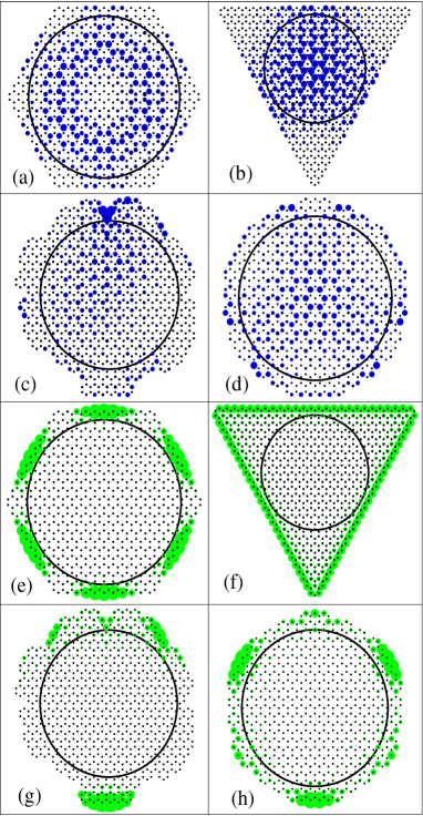
Figure 1: Amplitude of the wave function for bulk (a-d) and edge (e-h) states in GQD of different shapes. We also show the maximal inscribed circles that have been used to discern between bulk and edge states.

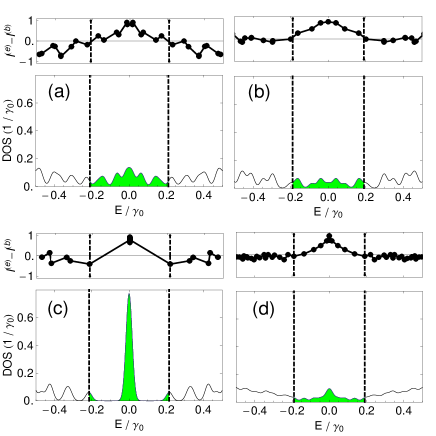
Figure 2: Electronic density of states and the difference of the edge and the bulk contributions intensities $I_{n}^{(e)}-I_{n}^{(b)}$ (see text) as a function of energy for the hexagonal (a), circular (b), triangular (c) and random (d) GQDs. The shaded region indicates the pseudogap where the edge states are located. The levels have been artificially shown as Gaussian peaks with the dispersion $0.05\mathrm{eV}$.

IV Hexagons, circles and random quantum dots

The susceptibility was calculated for zig-zag edge hexagons and circles of about of ten different sizes, having an inner radius in the range of $2-7\,\mathrm{nm}$. For random quantum dots, the averaging has been performed over three different ensembles, characterized by mean inner radii $R_{1}=2.6\,\mathrm{nm}$, $R_{2}=3.65\,\mathrm{nm}$ and $R_{3}=4.69\,\mathrm{nm}$. The magnetic field varied between 0 and $5\,\mathrm{T}$, range in which the susceptibility remained approximately constant. All the plots are presented for $B=5\,\mathrm{T}$. Fig. 2 shows the density of states as a function of Fermi energy for hexagonal and random-shape GQD. The shaded area indicates the region where the edge states are located.

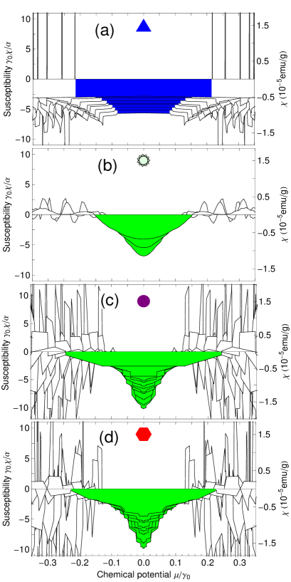
Figure 3: Susceptibility for triangular (a), random (b), circular (c) and hexagonal (d) GQDs of sizes $2-7\,\mathrm{nm}$. The shaded region indicates the (pseudo)gap.

Fig. 3 shows the magnetic susceptibility per unit of area as function of Fermi energy for GQD of different sizes. As was qualitatively explained above, the diamagnetic peak of width $2\Delta$ appears when the chemical potential crosses the pseudogap. This peak becomes wider with decreasing of GQD size. Beyond this zone, the orbital susceptibility is a highly fluctuating function of the Fermi energy that oscillates between paramagnetic and diamagnetic sign. These oscillations have been recently interpreted for graphene ribbons, as a result of the sub-band structure Ominato .

As it was mentioned above, the number of ZES for these geometries is vanishingly small that makes the diamagnetic contribution dominant for all sizes.

V Triangular quantum dots

All the edge states in triangular GQD with zig-zag edges are of ZES-type that do not change their energy as function of the field and do not contribute to the diamagnetic susceptibility. The ZES for GQD of different sizes are located in the middle of the gap $2\Delta$ as is shown in Fig. 4. We note that $2\Delta$ indicates the real gap in the spectrum for the triangular GQD, and the value of the this gap is inversely proportional to the number of ZES $\eta_{0}^{\Delta}$:

$$\Delta=\frac{\zeta\gamma_{0}}{\eta_{0}^{\Delta}}=\frac{\zeta\gamma_{0}}{\sqrt{(N+3)}-3},$$ (8)

where the numerical constant is $\zeta\simeq 5.56$.

The magnetic susceptibility of triangular GQD $\chi_{orb}^{\Delta}$ is shown in Fig. 3 for nine inner sizes of $2.5-7\,\mathrm{nm}$. It is provided by the out-of-gap delocalized electronic states and does not depend on $\mu$ within the gap $2\Delta$ because of absence of DES. These results match the analytical calculations of Ref. [Sharapov, ; Koshino2, ] for an infinite graphene sheet with the band gap $2\Delta$, according to which the diamagnetic susceptibility per unit area is

$$\chi_{\mathrm{orb}}^{\Delta}(\mu)=-\alpha\frac{\theta(\Delta-|\mu|)}{2\Delta},\qquad\alpha=\frac{e^{2}\gamma_{0}^{2}a^{2}}{2\pi\hbar^{2}c^{2}},$$ (9)

where $\theta(x)$ is the step function.

Although ZES give no contribution to the orbital susceptibility, they can be responsible for the huge paramagnetism provided by $\eta_{0}$ uncompensated electron spins located on the degenerate ZES levels. This happens in the case of small positive chemical potentials if the energy of electron-electron repulsion in each zero-energy state $U_{e-e}>\mu$, so that these levels remain half-filled. The corresponding Curie-type temperature-dependent paramagnetic susceptibility for non-interacting electrons is evaluated per unit area as

$$\chi_{\mathrm{spin}}^{\Delta}=\frac{\eta_{0}^{\Delta}}{\sigma}\frac{(g\mu_{B})^{2}}{3}\frac{s(s+1)}{k_{\mathrm{B}}T}=\frac{\eta_{0}^{\Delta}\mu_{B}^{2}}{\sigma k_{\mathrm{B}}T},$$ (10)

where $\mu_{B}$ is the Bohr magneton and $g\simeq 2$ is the g-factor of the electrons with spin $s=1/2$.

In the opposite case of the strong Coulomb electron correlations, according to the Lieb theoremLieb , all $\eta_{0}^{\Delta}\gg 1$ ZES electrons form the total spin of the cluster $S=\eta_{0}/2$. The super-paramagnetic susceptibility of ensemble of triangular GQD becomes even stronger,

$$\chi_{\mathrm{spin}}^{\prime\Delta}=\frac{1}{\sigma}\frac{(g\mu_{B})^{2}}{3}\frac{S(S+1)}{k_{\mathrm{B}}T}\simeq\frac{\left(\eta_{0}^{\Delta}\mu_{B}\right)^{2}}{3\sigma k_{\mathrm{B}}T}.$$ (11)

The actual value of paramagnetic susceptibility should be somewhere in between of $\chi_{\mathrm{spin}}^{\Delta}$ and $\chi_{\mathrm{spin}}^{\prime\Delta}$.

Using Eqs. (15) and (11) we compare the spin-paramagnetic and orbital-diamagnetic contributions, presenting their ratio for the case of strongly correlated electrons as

$$\left|\frac{\chi_{\mathrm{spin}}^{\prime\Delta}}{\chi_{\mathrm{orb}}^{\Delta}}\right|\simeq\frac{7.1eV}{\sqrt{N}k_{\mathrm{B}}\,T}.$$ (12)

It follows that varying the size and temperature of the triangular quantum dots, we can expect the paramagnetic-diamagnetic crossover. In particular, for a temperature of $T=77\,\mathrm{K}$, we predict that triangular quantum dots will be paramagnetic for the inner radius below $R\simeq 97\,\mathrm{nm}$.

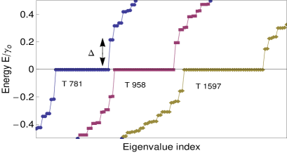
Figure 4: The band gap for triangular GQD with different number of atoms $N$.

VI Size Dependence

We calculated the gap-zone-integral $\int_{-\Delta}^{\Delta}\chi(\mu)d\mu$ of the shown in Fig. 3 diamagnetic susceptibilities for GQD of different shape and found that it preserves its intensity while the width $2\Delta$ vanishes as the size of GQD increases. In the limit of infinite cluster with $\Delta\rightarrow 0$ this gives the McClure $\delta$-peak of the graphene orbital susceptibility McClure1 :

$$\chi(\mu)=-\alpha\delta(\mu).$$ (13)

The shown in Fig.5 dependence of $\Delta$ on the number of atoms, is very similar for all shapes and follow the Eq.(8)

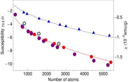
Figure 5: Pseudogap $\Delta$ dependence on the number of atoms in GQD of different geometry. The inset shows the energy dependence of susceptibility for a circular GQD with $N=709$

The size-dependence of the orbital susceptibility for hexagonal, circular and random GQDs at $\mu=0$ is shown in Fig.6. It satisfies an empirical relation

$$\chi_{orb}=\beta N^{\lambda}$$ (14)

with $\lambda=0.4$ and $\beta=0.31\alpha/\gamma_{0}$. Although the orbital diamagnetism is originated from the edge currents of the low-energy DES, their perimeter contribution $\sim N^{1/2}$ can be reduced by the armchair or/and zigzag type boundary irregularities as well as by the wave function vanishing at the corners of GQD that explains the reduction of the exponent index $\lambda$ slightly below $1/2$.

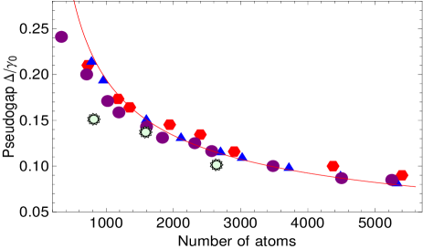
Figure 6: Dirac-point orbital susceptibility at $\mu=0$. The solid lines correspond to the fit according Eqs. (15) and (14).

For triangular GQD the size-dependence of the orbital susceptibility can be obtained by substituting the value of $\Delta$ from Eq.(8) into Eq.(9) at $\mu=0$:

$$\chi_{\mathrm{orb}}^{\Delta}=-\frac{\alpha}{\gamma_{0}}\frac{\sqrt{N+3}-3}{2\zeta}.$$ (15)

This estimation agrees with our numerical calculations as shown in Fig.6.

So far, there are no experimental measurements of magnetism of GQD but the susceptibility we obtained is in the range of the measured values for carbon nanotubes and buckyballs Bandow . For convenience we also presented the susceptibilities in Figs. 3 and 6 in the experimental units of emu/g.

VII Conclusions

Magnetism of GQD is provided by the edge states whose energy is located within the finite-size quantization pseudogap. The structure of the edge state spectrum and magnetic response of GQDs being strongly dependent on the geometric shape of the cluster.

For hexagonal, circular and random GQD the edge states are dispersed within the pseudogap. Their position depends on the applied field, providing the substantial diamagnetic response of GQD. The diamagnetic susceptibility as function of the chemical potential presents a peak of constant intensity, centered around $\mu=0$. The maximum of the peak increases with GQD size whereas its width decreases, approaching the $\delta$-function of McClure (13) for infinite sheet of graphene.

For triangular GQD the edge states are located exactly at the middle of the gap with the high degeneracy factor $\eta_{0}^{\Delta}$ given by Eq.(8) that increases with size of the cluster. The zero-energy position of these levels do not change with the field and the diamagnetic response of triangular GQD $\chi_{\mathrm{orb}}^{\Delta}$ is expected to be small. In a contrast, the uncompensated spins of electrons localized at ZES can provide the huge paramagnetic temperature-dependent contribution $\chi_{\mathrm{spin}}^{\Delta}$ of the Curie type. By comparison of susceptibilities $\chi_{\mathrm{orb}}^{\Delta}$ and $\chi_{\mathrm{spin}}^{\Delta}$, Eq.(12) we expect to have the crossover from paramagnetic to diamagnetic response in ensemble of triangular clusters with increasing the temperature and/or the GQD size.

The strong dependence of magnetic properties of GQDs on their geometry, size and temperature provides the natural way to separate the graphene clusters according to their shape and size by application of the appropriately designed non-uniform magnetic field and temperature cycle that can trap the different GQD in different points of space. It would be interesting also to study the specially cut nano-clusters of highly ordered pyrolytic graphite that can contain the separate graphene sheets with Dirac-like spectrum LukDirac and therefore can have the similar magnetic behavior.

References

- (1) J. Scott-Bunch et al., Nano Lett. 5, 287 (2005).
- (2) B. Ozyilmaz et al., Phys. Rev. Lett. 99, 166804 (2007).
- (3) W.L. Wang, O. V. Yazyev, S. Meng and E. Kaxiras, Phys. Rev. Lett. 102, 157201 (2009).
- (4) Z. Z. Zhang, K. Chang and F.M. Peeters, Phys. Rev. B 77, 235411 (2008).
- (5) S. Schnez, K. Ensslin, M. Sigrist, and T. Ihn, Phys Rev. B 78, 195427 (2008).
- (6) P. Potasz, A. D. Güçlü, and P. Hawrylak, Phys. Rev. B 81, 033403 (2010).
- (7) M. Zarenia, A. Chaves, G. A. Farias, and F. M. Peeters, Phys. Rev. B 84, 245403 (2011).
- (8) M. Grujic, M. Zarenia, A. Chaves, M. Tadic, G. A. Farias, and F. M. Peeters, Phys. Rev. B 84, 205441 (2011).
- (9) I. A. Luk’yanchuk and A. M. Bratkovsky, Phys. Rev. Lett., 100, 176404 (2008)
- (10) M. Ezawa, Phys. Rev. B 76, 245415 (2007).
- (11) J. Fernandez-Rossier and J.J. Palacios, Phys. Rev. Lett. 99, 177204 (2007).
- (12) W.L. Wang, S. Meng, and E. Kaxiras, Nano Lett. 8, 241 (2008).
- (13) J. W. McClure, Phys Rev. 104, 666 (1956).
- (14) J. W. Mc Clure, Phys Rev. 119, 606 (1960).
- (15) M. P. Sharma, L. G. Johnson, and J. W. McClure, Phys. Rev. B 9, 2467 (1974).
- (16) H. Fukuyama, J. Phys. Soc. Jpn. 76, 043711 (2007).
- (17) M. Nakamura, Phys Rev. B 76, 113301 (2007).
- (18) A. Ghosal, P. Goswami, and S. Chakravarty, Phys. Rev. B 75, 115123 (2007).
- (19) S. Slizovskiy and J. J. Betouras, Phys. Rev. B 86, 125440 (2012)
- (20) S. G. Sharapov, V. P. Gusynin and H. Beck, Phys. Rev. B 69, 075104 (2004)
- (21) K. Wakabayashi, M. Fujita, H. Ajiki, M. Sigrist, Phys. Rev. B. 59 8271 (1999).
- (22) M. Koshino and T. Ando, Phys. Rev. B 75, 235333 (2007).
- (23) J. Liu, Z. Ma, A. R. Wright an C. Zhang, J. Appl. Phys. 103, 103711 (2008).
- (24) M. Koshino and T. Ando, Phys. Rev. B 81, 195431 (2010).
- (25) Y. Ominato, M. Koshino, Phys. Rev. B 85, 165454 (2012).
- (26) K. Nakada, M. Fujita, G. Dresselhaus, M.S.Dresselhaus, Phys. Rev. B 54, 17954 (1996).
- (27) M. Fujita, K. Wakabayashi, K. Nakada, and K. Kusakabe, J. Phys. Sco. Jpn. 65, 1920 (1996).
- (28) J. Wurm, K. Richter and I. Adagideli, Phys. Rev. B 84, 075468 (2011).
- (29) H. P. Heiskanen, M. Manninen, and J. Akola, New J. Phys. 10, 103015 (2008).
- (30) T. Espinosa-Ortega, I. A. Luk’yanchuk, and Y. G. Rubo, Superlattices and Microstructures 49, 283 (2011).
- (31) A. V. Rozhkov, G. Giavaras, Y. P. Bliokh, V. Freilikher, and F. Nori, Physics Reports 503, 77 (2011).
- (32) S. Fajtlowicz, P. E. John and H. Sachs, Croat. Chem. Acta 78, 195 (2005).
- (33) Y. Ominato, M. Koshino, arXiv:1301.5440
- (34) E. H. Lieb, Phys. Rev. Lett. 62, 1201 (1989).
- (35) S. Bandow, J. Appl. Phys. 80, 1020 (1996).
- (36) I. Luk’yanchuk, Y. Kopelevich, and M. El Marssi, Physica B - Cond. Matt. 404, 404 (2009).