Protection of quantum states from disturbance due to random potential by successive translation

Abstract

We show a method to protect quantum states from the disturbance due to the random potential by successive rapid manipulations of the quantum states. The quantum states are kept undisturbed for a longer time than the case of the simple trapping with a stationary potential. The effective potential, which the quantum states feel, becomes uniform when the velocity of the transport is sufficiently large. It is also shown that the alternating transport of a Bose-Einstein condensate with the driving potential derived by fast-forward scaling theory [Masuda and Nakamura, Proc. R. Soc. A 466, 1135 (2010)] can protect it from the disturbance.

I Introduction

Technology to control quantum systems is rapidly evolving, and various methods to manipulate quantum states have been reported in Bose Einstein condensates (BEC)leg ; gus ; ket ; lea , in quantum computing nie and in many other fields of applied physics. For many current and future technologies the acceleration of controls of quantum systems would be important. Methods of the acceleration of quantum dynamics and quantum adiabatic dynamics or shortcut to adiabaticity have been proposed, e.g., counterdiabatic protocol ric and frictionless quantum driving ber3 , invariant-based inverse engineering mug1 and fast-forward scaling theory mas1 ; mas2 ; mas3 . These theories make possible to generate target states in short time without energy excitations at the final time of the manipulations muga_new . Recently applications of these methods to the controls of BEC including the transport have been proposed theoretically mug1 ; mas2 ; che ; mug2 ; torr ; Cam ; torr2 ; mas4 , and been demonstrated experimentally Scha ; Scha2 ; Bas . The robustness of these protocols have been investigated mas1 ; Che2 ; torr2 . In this paper we show a novel application and advantage of the acceleration of the quantum dynamics.

In actual systems there must be noise which prevents accurate controls of quantum systems. The influence of the random potential to the static and dynamical properties of the Bose-Einstein condensates (BECs) have been studied by using the optical speckle potential Lye ; For . The protection of quantum states from the influence of the noise and disorder would be an important issue as well as rapid controls for accurate manipulations of quantum states like BECs and for the extension of the range of the quantum controls. In this paper we use the random potential as the noise which deforms the wave function in a trapping potential neglecting the dissipation and decoherence due to the environment unlike the quantum decoupling of open systems Vio1 ; Vio2 . We show the protection of the quantum states from the disturbance due to the uncontrollable random potential in the background by rapid transport of the quantum states with the use of the fast-forward scaling theory. It is shown that the quantum states are kept undisturbed for a longer time than the case of the simple trapping with a stationary potential because the effective potential, which the quantum states feel, becomes uniform when the velocity of the transport is sufficiently large. It is numerically exhibited in one dimension that the alternating transport of a Bose-Einstein condensate can protect it from the disturbance.

In Sec.II we represent the model. And the driving potential for the adiabatic transport is reviewed. In Sec.III we show the protection of quantum states from the disturbance due to the random potential in the large-velocity-limit. In Sec.IV it is numerically exhibited that the fidelity is kept close to unity by the rapid one-way and alternative transports. The protection of a Bose-Einstein condensate is also shown numerically.

II Model

We consider a transport of a particle in one dimension. The driving potential for the ideal transport of quantum states without disturbance was derived, see e.g. mas2 . Suppose that $\Psi_{0}(x)$ is the wave function of an energy eigenstate trapped by the stationary potential $V_{0}(x)$ in the case without the random potential. The energy is assumed to be zero for the simplicity. The potential

$$\mathcal{V}(x,t)=V_{0}\big{(}x-R(t)\big{)}-\frac{d^{2}R(t)}{dt^{2}}mx.$$ (1)

can translates the quantum state without energy excitation at the final time of the manipulation mas2 . The change in $R(t)$ is the displacement of the trapping potential and the wave function. The first term in Eq.(1) corresponds to the translation of the trapping potential. The second term is the additional potential which is spatially linear. The wave function of the transported state $\Psi_{FF}$ is represented as

$$\Psi_{FF}(x,t) = \Psi_{0}\big{(}x-R(t)\big{)}$$ (2)

$$\times\exp\Big{[}i\dot{R}(t)\frac{m}{\hbar}x\Big{]},$$

where $\dot{R}$ denotes the time-derivative of $R$. $\dot{R}(t)$ is the velocity of the translation. $\Psi_{FF}(x,t)$ is a solution of the Schr$\ddot{\mbox{o}}$dinger equation:

$$i\hbar\frac{d\Psi_{FF}}{dt}=-\frac{\hbar^{2}}{2m}\frac{\partial^{2}\Psi_{FF}}{\partial x^{2}}+\mathcal{V}(x,t)\Psi_{FF}.$$ (3)

The additional phase in the wave function in Eq.(2) vanishes everywhere when the quantum state is stopped and $\dot{R}=0$.

Now we consider the translation under the random potential $V_{r}(x)$. We assume that the random potential is time-independent. In general the random potential can cause the disturbance of the wave function. The total Hamiltonian with the driving potential is represented as

$$H = \frac{p^{2}}{2m}+V_{0}\big{(}x-R(t)\big{)}$$ (4)

$$-\frac{d^{2}R(t)}{dt^{2}}mx+V_{r}(x).$$

In the following sections it is shown that the disturbance due to the random potential is restrained by the rapid transport.

III Analysis in large velocity limit

We show that the fast transport of the quantum states can reduce the influence of the random potential in the case of the constant velocity, $\dot{R}=v$, in the large-velocity-limit. In the analysis we use the moving frame which accompanies with the trapping potential. In the moving frame the third term in Eq.(4) vanishes and the Hamiltonian is represented by

$$H_{M}=\frac{p^{2}}{2m}+V_{0}(x)+V_{r}(x+vt).$$ (5)

The trapping potential is stationary in the moving frame while the random potential is moving with the constant velocity. We expand the state $\Psi$ by the energy eigenstates $|j>$ of the Hamiltonian: $H_{0}=p^{2}/2m+V_{0}(x).$ The state is represented as

$$|\Psi(t)>=\sum_{j}a_{j}(t)|j>,$$ (6)

where $H_{0}|j>=E_{j}|j>$ and $<j|k>=\delta_{jk}$. $E_{j}$ is the energy of the $j$th state. $|j>$ is time-independent. The Schr$\ddot{\mbox{o}}$dinger equation leads to the equations of the coefficients:

$$\partial_{t}a_{j}(t)=-\frac{i}{\hbar}E_{j}a_{j}(t)-\frac{i}{\hbar}\sum_{k}V_{jk}(t)a_{k}(t),$$ (7)

where $V_{jk}(t)$ is defined by

$$V_{jk}(t) \equiv <j|V_{r}(x+vt)|k>$$ (8)

$$= \int_{-\infty}^{\infty}\phi_{j}^{\ast}(x)\phi_{k}(x)V_{r}(x+vt)dx,$$

with $\phi_{j}(x)=<x|j>$. We suppose that the initial state is the $n$th energy eigenstate $|n>$, that is, $a_{j}(0)=\delta_{jn}$. $a_{j}(t)$ satisfies the integral equation:

$$a_{j}(t) = e^{-\frac{i}{\hbar}E_{j}t}\delta_{jn}$$

$$-\frac{i}{\hbar}\sum_{k}\int_{0}^{t}ds\ e^{-\frac{i}{\hbar}E_{j}(t-s)}V_{jk}(s)a_{k}(s).$$

For $m\neq n$ we obtain the 1st order approximation of $a_{m}(t)$ by substituting $j=m$ and the $0$th order solution $a_{k}(s)=\delta_{kn}\exp[-iE_{k}s/\hbar]$ in Eq.(LABEL:eq1_13_1) as

$$a_{m}(t) \simeq -\frac{i}{\hbar}\sum_{k}\int_{0}^{t}ds\ e^{-\frac{i}{\hbar}E_{m}(t-s)}$$ (10)

$$\times V_{mk}(s)e^{-\frac{i}{\hbar}E_{k}s}\delta_{kn}$$

$$= -\frac{i}{\hbar}e^{-\frac{i}{\hbar}E_{m}t}$$

$$\times\int_{0}^{t}ds\ e^{\frac{i}{\hbar}(E_{m}-E_{n})s}V_{mn}(s).$$

We assume that a finite number of the energy eigenstates can have the dominant contribution to the transition from the $n$th eigenstate in the 1st order approximation and the others are negligible because of the sufficiently small $V_{mn}$. Hereafter we focus on the energy eigenstates which may have the dominant contribution. We divide the time integral in Eq.(10) into the intervals as

$$\int_{0}^{t}ds=\int_{0}^{\Delta t}ds+\int_{\Delta t}^{2\Delta t}ds+\cdots+\int_{t-\Delta t}^{t}ds.$$

We take $\Delta t$ short enough so that $\exp[i(E_{m}-E_{n})s/\hbar]$ can be regarded as constant in the interval for any $m$, that is,

$$\omega_{mn}\Delta t\ll 1,$$ (12)

where $\omega_{mn}=(E_{m}-E_{n})/\hbar$. For example the $q$th integral with respect to $s$ of the last line in Eq.(10) is represented as

$$e^{\frac{i}{\hbar}\omega_{mn}q\Delta t}\int_{(q-1)\Delta t}^{q\Delta t}dsV_{mn}(s)$$

$$=e^{\frac{i}{\hbar}\omega_{mn}q\Delta t}\int_{(q-1)\Delta t}^{q\Delta t}ds\int_{-\infty}^{\infty}dx$$

$$\ \ \times\phi_{m}^{\ast}(x)\phi_{n}(x)V_{r}(x+vs)$$ (13)

The integration with respect to $s$ is rewritten with $\tau\equiv x+vs$ as

$$\int_{(q-1)\Delta t}^{q\Delta t}dsV_{r}(x+vs)$$

$$=\Delta t\frac{1}{v\Delta t}\int_{x+v(q-1)\Delta t}^{x+vq\Delta t}V_{r}(\tau)d\tau.$$ (14)

We define the effective potential $\bar{V}_{r}(x,q)$ by

$$\bar{V}_{r}(x,q)=\frac{1}{v\Delta t}\int_{x+v(q-1)\Delta t}^{x+vq\Delta t}V_{r}(\tau)d\tau,$$ (15)

which is the average of the random potential in the interval: $\Delta x=v\Delta t$. Suppose that $l$ is the length of $v\Delta t$ with which $\bar{V}_{r}(x)$ can be regarded as uniform in the region that wave function is localized. Thus if

$$v\Delta t>l,$$ (16)

we have

$$a_{m}(t)\simeq-\frac{i\Delta t}{\hbar}e^{-\frac{i}{\hbar}E_{m}t}\sum_{q}e^{i\omega_{mn}q\Delta t}$$

$$\times\int_{-\infty}^{\infty}dx\ \phi_{m}^{\ast}(x)\phi_{n}(x)\bar{V}_{r}(x,q)\simeq 0,$$ (17)

due to the orthogonality of $\phi_{n}$ and $\phi_{m}$. Therefore in the large $v$ limit, we see no transition among the energy eigenstates. From the conditions in Eqs.(12) and (16) We obtain a criterion of $v$:

$$v\gg\omega_{mn}l$$ (18)

with which the level transitions due to the random potential do not occur.

IV Numerical results

We numerically exhibit the protection of quantum states by the one-way translation with the constant velocity and the alternating translation in one dimension.

IV.1 Translation with constant velocity

We numerically simulate the transport with the constant velocity under the random potential. The fidelity of the quantum state is calculated during the time-evolution. We chose the trapping potential $V_{0}$ in Eq.(4) as the harmonic potential:

$$V_{0}(x)=\frac{m\omega^{2}}{2}x^{2}.$$ (19)

The initial state is taken as the ground state in the harmonic potential multiplied by a phase factor as

$$\Psi(x,0)=\Big{(}\frac{m\omega}{\pi\hbar}\Big{)}^{\frac{1}{4}}\exp\Big{[}{-\frac{m\omega}{2\hbar}x^{2}+i\dot{R}\frac{m}{\hbar}x}\Big{]},$$

(20)

where $\dot{R}$ is the velocity of the transport and is constant. $\Psi(x,t)$ is deformed from the exactly transported state $\Psi_{FF}(x,t)$ in Eq.(2) due to the random potential, while they coincide with each other at the initial time. The random potential has the rectangular form with the width $\eta$ as shown in Fig.1. The random potential takes the value from $-W/2$ to $W/2$.

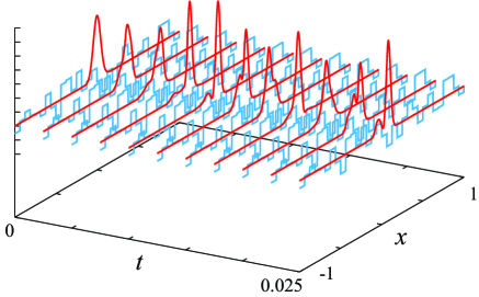
Figure 1: Snapshots of the time-evolution of $|\Psi|^{2}$ under random potential for $\dot{R}=0$. Red and blue lines correspond to $|\Psi|^{2}$ and the random potential, respectively. The parameters are taken as $m=1$, $\hbar=1$, $\omega=256$, $\eta=0.065$ and $W=1000$.

We drive the wave function in $x$-direction by moving the harmonic trap with the constant velocity (see Eq.(4)). In the numerical simulation we use the moving frame which accompanies with the trapping potential. The corresponding Hamiltonian is given by Eq.(5).

The snapshots of the time-evolution of $|\Psi|^{2}$ under random potential are shown in Fig.1 for $\dot{R}=0$ which corresponds to the simple trapping with the stationary potential. The harmonic potential is not shown in the figure. The parameters are taken as $m=1$, $\hbar=1$, $\omega=256$, $\eta=0.065$ and $W=1000$. The wave function is deformed due to the random potential. The time dependence of the fidelity is shown in Fig.2 for various values of $\dot{R}$. The fidelity is defined by $|<\Psi_{FF}(t)|\Psi(t)>|$ where $|\Psi_{FF}>$ in Eq.(2) is the exactly transported state without the disturbance of the random potential. The fidelity is averaged over the dynamics with 100 different random potentials. We see the decrease of the fidelity with time due to the disturbance by the random potential for $\dot{R}=0$. The fidelity for $\dot{R}=10$ and $30$ is lower than that of $\dot{R}=0$. This is because that the relative time-dependence of the random potential enhances the energy transition. However, for the sufficiently large velocity, $\dot{R}\geq 100$, the decrease of the fidelity is apparently restrained compared to the case of $\dot{R}=0$. The continuous transport reduces the influence of the random potential as theoretically predicted in the previous section. The variance of the fidelity is about 0.01 for $\dot{R}=100$. The variance tends to be smaller for larger $\dot{R}$.

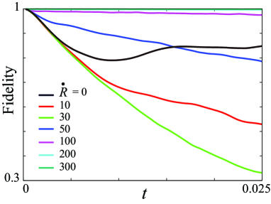
Figure 2: Time dependence of fidelity in one-way driving. The fidelity is averaged over the dynamics with 100 different random potentials. $\dot{R}$ is the velocity of the centre of trapping potential. Other parameters are the same as Fig.1.

$\bar{V}_{r}$ in Eq.(15) is regarded as the effective potential that the quantum state feels. To show the property of the effective potential we calculate

$$V_{eff}(x,\delta l)\equiv\frac{1}{\delta l}\int_{x}^{x+\delta l}V_{r}(\tau)d\tau,$$ (21)

which corresponds to $\bar{V}_{r}$ for $q=0$. The distance $\delta l$ corresponds to $v\Delta t$. The effective potential $V_{eff}(x,\delta l)$ for the various values of $\delta l$ are shown in Fig.3.

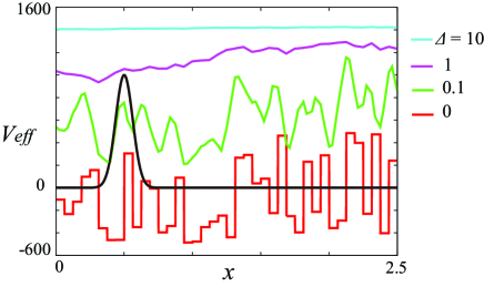
Figure 3: Effective potential $V_{eff}(x,\delta l)$ for $\delta l=0,0.1,1,10$. $V_{eff}$ for $\delta l>0$ are shifted upward for the comparison. Other parameters are the same as Fig.1.

For large $\delta l$ ($\delta l=1$ and $10$) the effective potential become smooth and uniform compared to the original random potential. This property of the effective potential explains the decrease of the influence of the random potential. The distance $\delta l=1$ corresponds to $\dot{R}=256$ if we relate the distance $\delta l$, the time-interval $\Delta t$ and the frequency $\omega$ by $\delta l=\dot{R}\Delta t$ and $\Delta t=1/\omega$.

IV.2 Alternating translation

In actual systems it is impossible to keep translating the quantum state in one direction. Here we show that the alternating translation also protects quantum states from the disturbance due to the random potential in one dimension. The trapping potential $V_{0}(x)$ is the harmonic potential as Eq.(19), and the initial state is the ground state given by Eq.(20) with $\dot{R}=0$. We choose the time dependence of $R(t)$ as

$$R(t)=\frac{L}{2}\{1-\cos(\omega_{R}t)\}.$$ (22)

We continuously translate the quantum state back and forth by translating the trapping potential and simultaneously tuning the spatially linear potential as Eq.(1). The center of the wave packet is oscillated between $x=0$ and $x=L$ periodically. The random potential is the same as Sec.IV.1. In the numerical simulation we use the moving frame which accompanies with the original trapping potential $V_{0}$.

The time dependence of the fidelity is shown in Fig.4 for various values of $\omega_{R}$. The corresponding value of the time-average of $|\dot{R}|$ denoted by $<|\dot{R}|>$ are shown in the figure. We put $L=2$. Other parameters are the same as Fig.1. The fidelity is averaged over the dynamics with 100 different random potentials. The variance of the fidelity is about 0.015 for $<|\dot{R}|>=4000$. The variance tends to be smaller for larger $<|\dot{R}|>$. It is seen that the alternating translation with the sufficiently large frequency can reduce the influence of random potential. The rapid falls of the fidelity occur at the time when the trapping potential is turned and starts to move in the opposite direction. Since the velocity becomes small at such time, the quantum state is affected by the random potential and the fidelity decreases.

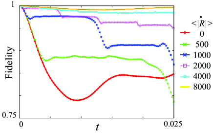
Figure 4: Time dependence of fidelity in the alternating translation for various values of $<|\dot{R}|>$. The fidelity is averaged over the dynamics with 100 different random potentials. Other parameters are the same as Fig.1.

IV.3 Bose-Einstein condensates

Here we apply the method to reduce the influence of the random potential to Bose-Einstein condensates (BECs). We assume that the system is governed by the Gross-Pitaevskii (GP) equation:

$$i\hbar\frac{d\Psi}{dt}=-\frac{\hbar^{2}}{2m}\frac{\partial^{2}\Psi}{\partial x^{2}}+\mathcal{V}(x,t)\Psi+c|\Psi|^{2}\Psi,$$

where $\Psi(x,t)$ is the macroscopic wave function, and $c$ is the coupling parameter. It has been shown that the BECs are also transported without energy excitation by the same driving potential in Eq.(1) mas2 ; torr3 ; mas4 . Let us suppose that a BEC wave packet is trapped by the harmonic potential subjected to the random potential which is the same as the previous sections. The initial state is the ground state obtained numerically in the stationary harmonic potential without the random potential. We alternately translate the wave packet by using the driving potential. The time dependence of $R(t)$ and the parameters are same as Sec.IV.2. In Fig.5 the time dependence of the fidelity is shown for $c=10$. The fidelity shows the similar time-dependence to the case with $c=0$. The results show that the disturbance of BECs can be suppressed by the repeated driving of the wave packet.

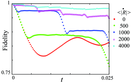
Figure 5: Time dependence of fidelity in alternating translation for $c=10$. Other parameters are the same as Fig.4.

V summary and discussion

We have presented the protection of quantum states from the disturbance due to the random potential by the continuous transport with the use of the driving potential derived by the theory of the acceleration of adiabatic dynamics. We analytically showed that the fast translation of the quantum states can suppress the influence of the random potential because the effective potential which the quantum states feel becomes uniform when the velocity of the transport is sufficiently large. We emphasize that the velocity of the transport does not have to be fast enough so that the effective potential vanishes.

We have numerically exhibited the protection of the quantum states by the continuous translation with the constant velocity and the alternating translation of the the ground state in the harmonic potential. The decrease of the fidelity is clearly restrained by the fast-driving compared to the simple trapping with a stationary potential, while the protection effect is not monotonously increased with the velocity in the small-velocity-region. It has been shown that the same technique is effective also for the protection of BECs from the influence of the random potential.

The optical speckle potential were used to investigate the properties of BECs under the random potential experimentally Lye ; For . It is expected that such system would be useful to investigate the present method experimentally because the strength of the random potential can be controlled by tuning the intensity of the laser. In this paper we did not consider the dissipation and decoherence effects. Applications of the present method in the system with the dissipation and decoherence would be studied in the future also with the effect of the time-dependence of the random potential. We assumed that the driving potential is controlled without error, while for rapid manipulation the control of the potential itself can cause additional noises in actual systems. The investigation of the robustness of the present technique is a future issue.

- (1) A. J. Leggett, Rev. Mod. Phys. 73, 307 (2001).
- (2) T. L. Gustavson, A. P. Chikkatur, A. E. Leanhardt, A. Grlitz, S. Gupta, D. E. Pritchard and W. Ketterle, Phys. Rev. Lett. 88, 020401 (2001).
- (3) W. Ketterle, Rev. Mod. Phys. 74, 1131 (2002).
- (4) A. E. Leanhardt, A. P. Chikkatur, D. Kielpinski, Y. Shin, T. L. Gustavson, W. Ketterle and D. E. Pritchard, Phys. Rev. Lett. 89, 040401 (2002).
- (5) M. A. Nielsen and I. L. Chuang, Quantum computation and quantum information (Cambridge Univ. Press, Cambridge, UK, 2000).
- (6) M. Demirplak and S. A. Rice, J. Phys. Chem. 107, 9937 (2003).
- (7) M. V. Berry, J. Phys. A 42, 365303 (2009).
- (8) J. G. Muga, X. Chen, A. Ruschhaupt and D. Guéry-Odelin, J. Phys. B 42, 241001 (2009).
- (9) S. Masuda and K. Nakamura, Phys. Rev. A 78, 062108 (2008).
- (10) S. Masuda and K. Nakamura, Proc. R. Soc. A 466, 1135 (2010).
- (11) S. Masuda and K. Nakamura, Phys. Rev. A 84, 043434 (2011).
- (12) J. G. Muga, arXiv:1212.6343 (2012).
- (13) X. Chen, A. Ruschhaupt, S. Schmidt, A. del. Campo, D. Guéry-Odelin and J. G. Muga, Phys. Rev. Lett. 104, 063002 (2010).
- (14) J. G. Muga, X. Chen, S. Ibáez, I. Lizuain and A. Ruschhaupt, J. Phys. B 43, 085509 (2010).
- (15) E. Torrontegui, S. Ibáez, X. Chen, A. Ruschhaupt, D. Guéry-Odelin and J. G. Muga, Phys. Rev. A 83, 013415 (2011).
- (16) A. del Campo, Eur. Phys. Lett. 96, 60005 (2011).
- (17) E. Torrontegui, X. Chen, M. Modugno, S. Schmidt, A. Ruschhaupt, D. Guéry-Odelin and J. G. Muga, New J. Phys. 14, 013031 (2012).
- (18) S. Masuda and K. Nakamura, Phys. Rev. A 86, 063624 (2012).
- (19) J.-F. Schaff, X. -L. Song, P Vignolo, and G. Labeyrie Phys. Rev A 82, 033430 (2010).
- (20) J.-F. Schaff, X.-L. Song, P. Capuzzi, P. Vignolo and G. Labeyrie, Eur. Phys. Lett. A 93, 23001 (2011).
- (21) M. G. Bason, M. Viteau, N. Malossi, P. Huillery, E. Arimondo, D. Ciampini, R. Fazio, V. Giovannetti, R. Mannella and O. Morsch, Nat. Phys. 8, 147 (2011).
- (22) X. Chen, E. Torrontegui, D. Stefanatos, J. Li, and J. G. Muga, Phys. Rev. A 84, 043415 (2011).
- (23) J. Lye, L. Fallani, M. Modugno, D. Wiersma, C. Fort, M. Inguscio, Phys. Rev. Lett. 95, 070401 (2005).
- (24) C. Fort, L. Fallani, V. Guarrera, J. Lye, M. Modugno, D. Wiersma, and M. Inguscio Phys. Rev. Lett. 95, 170410 (2005).
- (25) L. Viola and S. Lloyd, Phys. Rev. A 58, 2733 (1998).
- (26) L. Viola and S. Lloyd, Phys. Rev. Lett. 82, 2417 (1999).
- (27) E. Torrontegui, S. Martínez-Garaot, A. Ruschhaupt and J. G. Muga, Phys. Rev. A 86, 013601 (2012).